
 Submit a Paper
 Propose a Special lssue
 Open Access
ARTICLE

A Multi-Attribute Decision-Making Method Using Belief-Based Probabilistic Linguistic Term Sets and Its Application in Emergency Decision-Making
School of Management, Harbin Institute of Technology, Harbin, 150001, China
* Corresponding Author: Liguo Fei. Email:
(This article belongs to the Special Issue: Linguistic Approaches for Multiple Criteria Decision Making and Applications)
Computer Modeling in Engineering & Sciences 2023, 136(2), 2039-2067. https://doi.org/10.32604/cmes.2023.024927
Received 14 June 2022; Accepted 21 September 2022; Issue published 06 February 2023
 View Full Text
 Download PDF
Abstract
Probabilistic linguistic term sets (PLTSs) are an effective tool for expressing subjective human cognition that offer advantages in the field of multi-attribute decision-making (MADM). However, studies have found that PLTSs have lost their ability to accurately capture the views of decision-makers (DMs) in certain circumstances, such as when the DM hesitates between multiple linguistic terms or the decision information is incomplete, thus affecting their role in the decision-making process. Belief function theory is a leading stream of thought in uncertainty processing that is suitable for dealing with the limitations of PLTS. Therefore, the purpose of this study is to extend PLTS to incorporate belief function theory. First, we provide the basic concepts of the extended PLTS (i.e., belief-based PLTS) through case analyses. Second, the aggregation operator of belief-based PLTS is defined with the ordered weighted average (OWA)-based soft likelihood function, which is improved by considering the reliability of the information source. Third, to measure the magnitude of different belief-based PLTSs, the belief interval of singleton is calculated, and the comparison method of belief-based PLTS is constructed based on probabilities. On the basis of the preceding discussion, we further develop an emergency decision framework that includes several novel techniques, such as attribute weight determination and decision information aggregation. Finally, the usefulness of the framework is demonstrated through a case study, and its effectiveness is illustrated through a series of comparisons.Graphic Abstract
Keywords
Emergencies of various types are occurring increasingly frequently in the modern interconnected world, which is a phenomenon that has attracted great public attention [1]. Emergencies are characterized by complexity, uncertainty and a high degree of destructiveness. Their occurrence causes great harm in terms of both public health and property damage [2]. Proper awareness of disasters and effective coping strategies can help the public respond such that they do not become life-threatening [3]. Therefore, actively engaging in disaster prevention education is of great significance in minimizing the damage caused by disasters [4].
Choosing a multiple-disaster risk reduction education plan is an emergency decision problem and therefore essentially a multi-attribute decision problem [5]. Due to the randomness, multi-dimensionality and uncertainty of emergency decision-making, a disaster risk reduction education plan should also consider the complexity of the decision environment [6]. Decision makers are the main participants in emergency decision-making, and their professional knowledge and experience play a key supporting role in evaluating events as they occur. Therefore, human subjectivity will inevitably be a factor in emergency decision-making. To avoid the decision error caused by fuzziness and uncertainty, a wide variety of information expression methods have been proposed to capture DMs’ subjectivity, such as the intuitionistic [7,8], hesitant [9,10], and Pythagorean fuzzy sets [11], among others.
Because of the lack of accurate information and the environmental uncertainty-as well as the urgency to make a decision-linguistic information and judgment are often employed as they represent the only means through which to represent DMs’ point of view in linguistic terms, such as
Since PLTSs were first proposed in [13], the research on PLTS and MADM based on PLTS has attracted considerable attention. Liao et al. [14] proposed a comprehensive approach for multi-expert MADM problems that considers both quantitative and qualitative criteria and has been implemented to address green enterprise ranking issues. Jiang et al. [15] combined PLTS and the fuzzy least absolute regression to construct a fuzzy regression model capable of handling mixed types of inputs. Nie et al. [16] developed a group decision-making support model using prospect theory-based consistency recovery strategies based on PLTS. Wang et al. [17] extended TOPSIS, VIKOR and TODIM methods based on PLTS to be applicable to multi-expert MADM issues. An integrated MADM method based on PLTS was presented in [18] to determine the best medical product supplier. Li et al. [19] applied PLTS to determine variable weights in solving multi-attribute two-sided matching problems. To evaluate web celebrity shops, Liang et al. [20] employed long short-term memory and PLTSs to describe customers’ satisfaction. Several novel aggregation operators of PLTSs were defined in [21] to solve multi-attribute group decision-making problems. A MADM model was presented in [22] based on incomplete dual probabilistic linguistic preference relations to help enterprises select their 5G partners.
Although traditional PLTSs have been applied to different types of decision problems, the existing approaches show certain limitations and weaknesses, which are reflected in three aspects. The first is in terms of information expression. As probability information is often incomplete, normalization is required in order to fill any gaps in the data [13,23,24]. Second, it only allows for the distribution of probabilities on the singleton and cannot express situations in which the DM hesitates over two or more linguistic terms [24–26]. Third, the PLTS-based decision methods mostly fail to consider the missing attribute values, which are often unavoidable in practice [12,27,28]. In terms of information aggregation, aggregation operators based on the traditional Dempster’s fusion rule or ER method may suffer from information explosion caused by too many linguistic terms, which implies that the complexity of the algorithm needs to be reduced. In terms of decision-making processes, there is no research on the extension of belief-based PLTSs to emergency management issues, and any related studies do not provide a complete decision-making framework. By recognizing these limitations, the motivation of this study is to overcome these defects to make PLTSs more applicable to long-term decision-making. In particular, as decision environments in many applications, such as responding to major emergencies, are highly uncertain and complex, more powerful tools are needed in order to capture how DMs evaluate information. To achieve such a goal, this paper proposes and develops an uncertain information representation and processing method using belief function theory [29,30], which has been widely used in information fusion [31–34] and decision-making [35–37].
In short, the purpose of this study is to extend PLTS by incorporating belief function theory to make it more flexible in terms of expressing opinions. The innovations of this paper can be summarized as follows:
• The new concept of belief-based PLTS is first introduced, and then the composition of its belief interval is proposed, which includes the belief and plausibility functions. Several examples are provided to facilitate understanding of how the extended belief-based PLTS is used.
• The novel aggregation operator for belief-based PLTS is proposed using an OWA-based soft likelihood function, which can effectively describe DMs subjective attitudes, and the aggregation process is demonstrated using numerical examples. The aggregation operator is upgraded by considering the reliability of information sources, and the aggregation process is demonstrated using numerical examples.
• To compare different belief-based PLTSs, a novel possibility degree method is defined based on the belief interval of the singleton. An illustrative example is provided to demonstrate how to determine the sizes of different belief-based PLTSs.
• Based on the proposed belief-based PLTS and its corresponding operations, a multi-attribute decision-making framework is constructed and applied to emergency decision-making, and the detailed process is developed and explained step by step.
To illustrate the applicability of the proposed approach and verify its usefulness, a complete case study is presented based on the defined emergency decision methodology for selecting the best emergency risk education program. Decision results and comparative analysis are given to demonstrate the usefulness and effectiveness of the method proposed in this paper.
The study is carried out according to the following organization. In Section 2, we introduce some preliminaries, including probabilistic linguistic term set, belief function theory, and OWA operator. In Section 3, we explore extending PLTS with belief function theory, introducing basic concepts, aggregation operators, and comparison function. In Section 4, we provide a framework for multi-attribute decision making and apply it to emergency decision problems. In Section 5, we give a case study to demonstrate the usefulness and effectiveness of the proposed emergency decision method. In Section 6, we summarize this study and provide future research.
Some basic prerequisites are introduced in this section, including linguistic term set, probabilistic linguistic term set, belief function theory, and OWA operator.
In practical decision problems, the linguistic term set is very common and useful, because it is more in line with the DM’s habit of thinking [38]. A subscript-symmetric linguistic term set is defined as
•
•
• the negation operator of
2.2 Probabilistic Linguistic Term Set (PLTS)
Probabilistic linguistic term set was presented by Pang et al. [13] to address the weakness that all linguistic term sets in hesitant fuzzy linguistic term set (HFLTS) have the same weight. To demonstrate the shortcomings of HFLTS, and to emphasize the need to introduce PLTS, an illustrative example is presented.
Example 1. In a serious mine accident, the DMs need to evaluate the emergency plans. With regard to an emergency plan
which is not appropriate for HFLTS.
From the above example it can be concluded that the assessment information is expressed not only as a set of possible linguistic terms but also as their corresponding probabilities. To effectively express the opinions of DMs, the probabilistic linguistic term set is proposed and defined as follows:
Definition 2.1. [13] Let
where
Based on the above definition, we can represent the evaluation information in Example 1 by a PLTS as
Definition 2.2. [13] Let two normalized PLTSs be represented as
• If
• If
– If
– If
Definition 2.3. [13] Let a normalized PLTS be
where
Definition 2.4. [13] Let a normalized PLTS be
The theory of belief function is an uncertain reasoning one initiated by Dempster [29] and inherited and developed by Shafer [30], therefore also known as Dempster-Shafer theory (DST). After half a century of development, the theory has been well developed and played an important role in a wide variety of fields, such as decision-making [40–42] and information fusion [43–45]. Suppose that the answer to the question of concern consists of a finite set of mutually exclusive elements, called frame of discernement (FoD), expressed as
Definition 2.5. The belief function
And we have
Definition 2.6. The plausibility function
where
OWA operator, originally introduced by Yager et al. [48–50], is an information aggregation method between the maximum and minimum operators.
Definition 2.7. [48] Let
where
Definition 2.8. [48] OWA operators are highly dependent on weighting vector
•
•
•
•
Definition 2.9. The weighting vector for OWA operator can be determined as
where f is a monotonic function that satisfies
In [51], a useful function
Note that the larger attitudinal character
3 Belief-Based Probabilistic Linguistic Term Sets
In this section, the belief-based probabilistic linguistic term sets are developed to overcome the issues of PLTSs by expressing and dealing with more uncertainty. We first give the basic concept of belief-based PLTSs, then provide the aggregation operator and finally define the score function in order to effectively complete the emergency decision-making process.
The probabilistic linguistic term set effectively solves the problem that the HFLTS cannot assign weight to the possible linguistic terms according to the DM’s preference. However, the PLTS has also been criticized for its limitations in decision-making [28]. According to Definition 2.1, PLTS allows probability information to be incomplete, but other operations of the PLTS can only be performed after the probability is normalized. Allowing incomplete information expression is conducive to contain more uncertainty, but the normalization for subsequent calculations directly distributes the uncertainty to each linguistic term, which artificially removes some unknown uncertainties and weakens the effectiveness of the modeling uncertainty.
In complex decision-making, especially emergency problems, there may be various uncertainties, including randomness, vagueness and incompleteness [52]. Randomness comes from non-deterministic conditions, ambiguity is caused by unclear classification of things, and incompleteness is caused by incomplete information. PLTS has some potential limitations in the expression of uncertainty, such as the aforementioned normalization problem, the inability to express simultaneity, and the lack of attribute values that are not considered. The belief function theory is a powerful tool for expressing and dealing with uncertainty, which has been widely declared and recognized by authoritative literature [29,34,35,46]. In order to solve the potential limitation of PLTS in MADM, the concept of belief-based PLTS is introduced.
For instance, in Example 1, the evaluation is represented by PLTS as
where S is FoD, indicating unknown or uncertain.
It is worth noting that incompleteness of information is also seen in another scenario in decision making. For example, in multi-attribute emergency decision making, the DM has completed the evaluation of the performance of an emergency plan under other attributes, but only in the aspect of attribute “response speed” is unknown. The traditional PLTS-based emergency decision making method rarely considers this situation, which leads to the interruption of the emergency procedure. Within the frame of belief function theory, the missing attribute value can be represented as
Another motivation that we have to extend PLTS with belief function theory is to deal with a decision scenario where a DM is hesitant between two or more linguistic terms. In other words, the probability distribution on the single term no longer meets the expression requirements of DMs, but needs to allocate the belief on multiple subsets. Take the decision scenario in Example 1, where 80 experts evaluate it “good”, 10 evaluate it “medium”, and 10 hesitate between the terms “good” and “medium”. Obviously, PLTS is powerless to describe this case, but the theory of belief function can handle and represent such a case well with the expression
Through the above analysis and discussion, we identify some limitations of PLTS in expressing DMs’ views, and analyze the advantages of belief function theory in solving these problems. This is therefore an appropriate time to present the belief-based probabilistic linguistic term set as below:
Definition 3.1. Let
where
Based on Definition 3.1, the evaluations in Eqs. (15) and (16) can be represented by belief-based PLTSs as
Definition 3.2. The belief function of belief-based PLTS
And we have
Definition 3.3. The plausibility function of belief-based PLTS
where
3.2 A Novel Aggregation Operator for Belief-Based PLTS
In decision problems, an aggregation operator is inevitably employed, which is an approach combining two or more single information expressions. The above manifests the advantages of the belief-based PLTS in representing uncertain information. To make it exert maximum in decision making, this section provides a novel aggregation operator for belief-based PLTS ground on soft likelihood function.
Soft likelihood function was originally proposed by Yager et al. [53] for calculating likelihood functions of probabilistic evidence in the context of forensic crime investigations. It breaks the limitations of traditional likelihood functions that use logical “anding” to aggregate elements, and has been extended to uncertain decision environments by D numbers [54], power OWA [55,56], and Pythagorean fuzzy sets [57,58]. With the flexible and reliable combination ability of soft likelihood function, in this section, an aggregation operator for belief-based PLTS is proposed.
Definition 3.4. Let
The above definition multiplies the belief of
Definition 3.5. Let
where
Definition 3.6. The OWA-based soft likelihood function of
where
According to Definition 2.8, we analyze the OWA-based soft likelihood function corresponding to the special forms of weight distribution.
• For
• For
• For
Definition 3.7. Based on Definition 2.9, the attitudinal character
To ensure that the aggregated result is still a belief-based PLTS, it needs to be normalized as
Therefore, the aggregation operator of n belief-based PLTSs can be defined as
To demonstrate the usage of the above-proposed aggregation operator, the following example is given.
Example 2. Let
According to Definition 3.5, the product of the j largest belief of
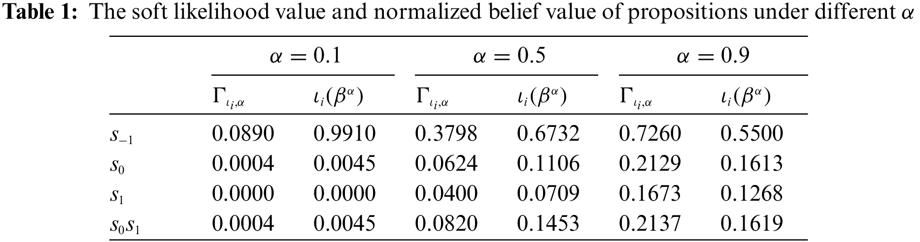
Now we discuss the soft likelihood value of
• When
• When
• When
According to the above process, soft likelihood values of other propositions (
3.3 The Aggregation Operator Considering the Reliability of Belief-Based PLTS
In practical decision problems, different belief-based PLTSs generally have different importance, i.e., weight, also known as reliability. The aggregation operator proposed in the previous section assumes that all belief-based PLTSs have the same reliability, which leads to certain limitations in decision making. To solve this problem, this section develops an aggregation operator considering reliability.
From the definitions in the previous section, it can be concluded that the advantages of soft likelihood function-based aggregation operator mainly come from two aspects: cumulative multiplication and OWA. Reliability will affect the order determination and weight vector generation.
Definition 3.8. The reliability of
where
Definition 3.9. The OWA-based soft likelihood function of
where
Definition 3.10. To determine the OWA weighting vector, the sum of reliability of the j largest
Consequently, the OWA weighting vector of the soft likelihood function considering reliability can be defined as
Note that if the reliability of all belief-based PLTSs is equal, i.e.,
Definition 3.11. The aggregation operator of n belief-based PLTSs considering reliability is defined as
where
The case in Example 2 is used to demonstrate the aggregation operator considering reliability.
Example 3. Let the reliability of
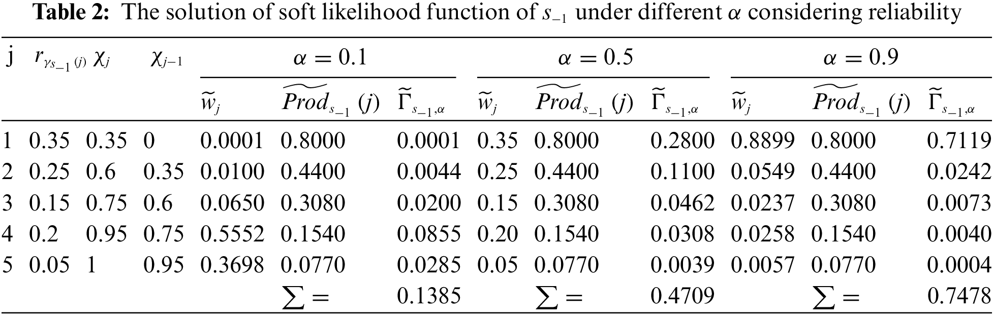
According to the above process, soft likelihood values of other propositions (
In Examples 2 and 3, we present several special cases to reflect the impact of parameter
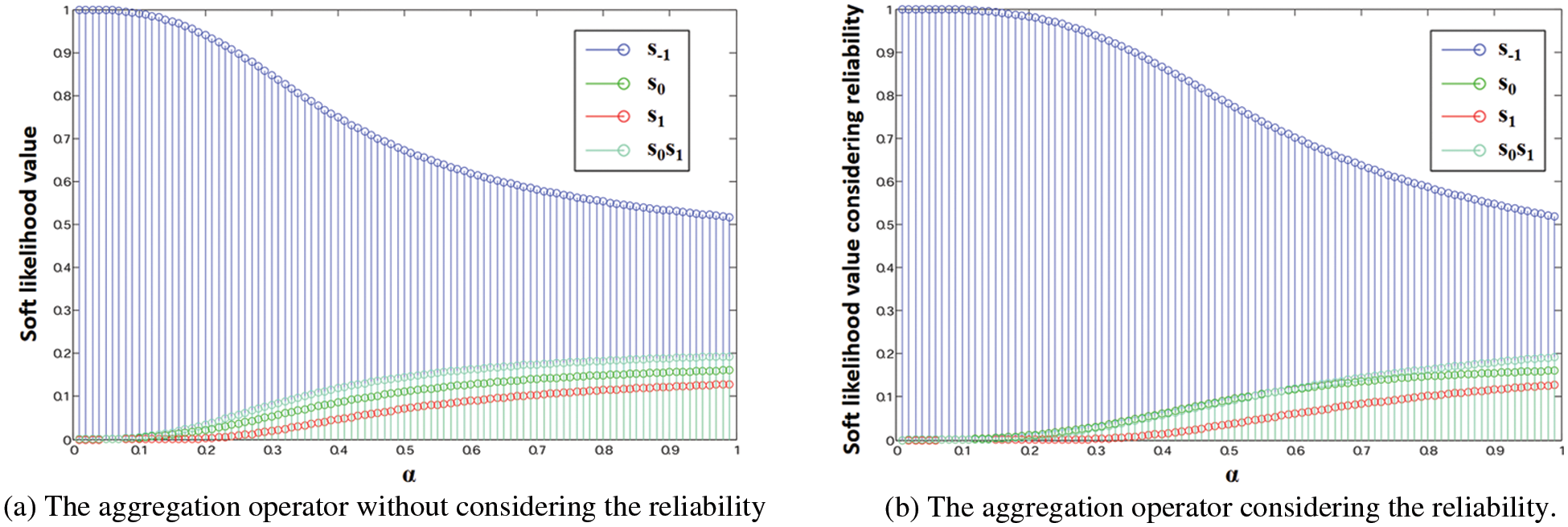
Figure 1: The belief distribution of the aggregated belief-based PLTS with different
3.4 The Comparison between Belief-Based PLTSs
Belief-based PLTS is a new expression of uncertainty based on linguistic information. Due to its complexity, it is not easy to define score functions like PLTS. Therefore, by virtue of belief interval, we propose a novel possibility degree method for comparing belief-based PLTSs.
Definition 3.12. Let
where
Definition 3.13. Let
Definition 3.14. Let
where
Based on above definitions, under the assumption that
Theorem 3.1.
Theorem 3.2.
Theorem 3.3.
Theorem 3.4.
The above theorems are obvious, so the proof is omitted. Definition 3.14 provides the possible degree calculation method for two belief-based PLTSs sorting, and we further extend it to the scenario of n belief-based PLTSs.
Definition 3.15. Let a set of belief-based PLTSs with n elements be represented as
which can be employed to sort
The belief-based PLTSs in Example 2 are used to be sorted by using the above method in this section.
Example 4. We take
Then the score of
So the scores of
According to Definition 3.15, the sort value of the belief-based PLTSs can be calculated as
4 Emergency Decision-Making Based on Belief-Based Probabilistic Linguistic Term Sets
In recent years, various unconventional emergencies have occurred frequently, which has become a major risk and disaster facing mankind. How to reduce the loss caused by a disaster and carry out effective rescue work based on emergency decision methods has become an important step in dealing with emergencies. In this section, we propose a multi-attribute decision making method for emergency decision based on the defined belief-based PLTS.
In a multi-attribute emergency decision making problem, the alternative set is
where
4.2 Aggregation of Decision Information of Experts
After obtaining the experts’ decision matrices, the opinions need to be aggregated first. For the comprehensive performance of alternative
where
4.3 Determination of Attribute Weight
The methods for determining attribute weights can be divided into the subjective, objective and combination weighting methods. The last method combines the characteristics of the former two, avoids the subjective arbitrariness, and captures the preference of DMs for the attribute. Therefore, based on the defined belief-based PLTS, this paper proposes a combination weighting method which aggregates both subjective and objective.
4.3.1 Determination of Subjective Weight Based on Belief-Based PLTSs
Humans are at a loss when asked to compare multiple attributes. But it is much easier for humans to compare pairs of attributes, an idea that has been repeated in the AHP and BWM approaches [60]. Based on this consideration, we propose a method to determine the subjective weight of attributes.
Let the set of attributes be represented as
Definition 4.1. For a given belief-based PLTS
where
To demonstrate how to use the defined negation of belief-based PLTSs, the following example is given.
Example 5. The pairwise comparison between
• Case 1: when
• Case 2: when
• Case 3: when
A pairwise comparison matrix
4.3.2 Determination of Objective Weight Based on Interval Entropy Weight Method
The basic idea of the entropy weight method is to determine the objective weight according to the magnitude of the attribute variability. Generally, entropy is employed to reflect uncertainty. In decision-making problems, the lower the entropy, the greater the uncertainty, the greater the degree of variation of the attribute, the greater the degree of differentiation, and the greater the weight, and vice versa.
For decision matrix
To make all the values participating in the normalization positive, the scores will be shifted to ensure that the minimum lower limit of the interval values corresponding to each attribute is 0. The interval entropy weight method is carried out in the following steps.
Step 1: Normalize data. Since there may be negative numbers in the matrix, we first translate the data to get
Step 2: Calculate the entropy of
Step 3: Calculate the diversification of
Step 4: Obtain the objective weight
4.3.3 Determination of Final Weight by Combining Subjectivity and Objectivity
The subjective weight
4.4 Decision Information Aggregation
Based on the attribute weights obtained in the previous subsection and the decision matrix in Eq. (40), the evaluations of alternative
Definition 4.2. Let the interval weight of attribute
where
The normalized weight representative value defined above can be considered as the reliability of the attribute, then different attribute values can be aggregated based on the aggregation operator in Section 3.2.
Definition 4.3. Let the belief-based PLTSs of alternative
4.5 Calculation of the Final Ranking of Alternatives
According to the aggregated results, the final ranking of alternatives can be calculated by comparing the corresponding belief-based PLTSs. Let the belief-based PLTSs of alternative
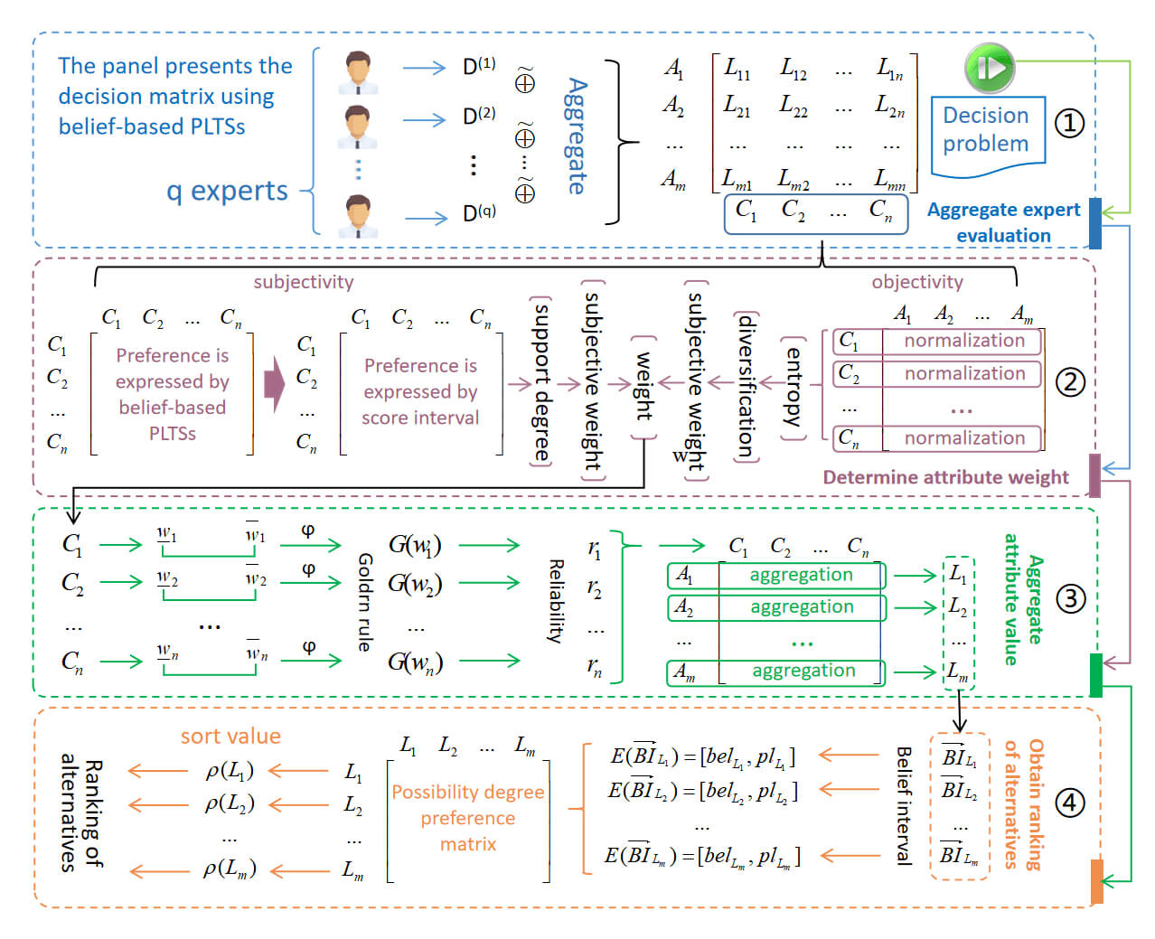
The above proposed approach can be summarized as the emergency decision-making framework based on belief-based probabilistic linguistic term sets as shown in Fig. 2.
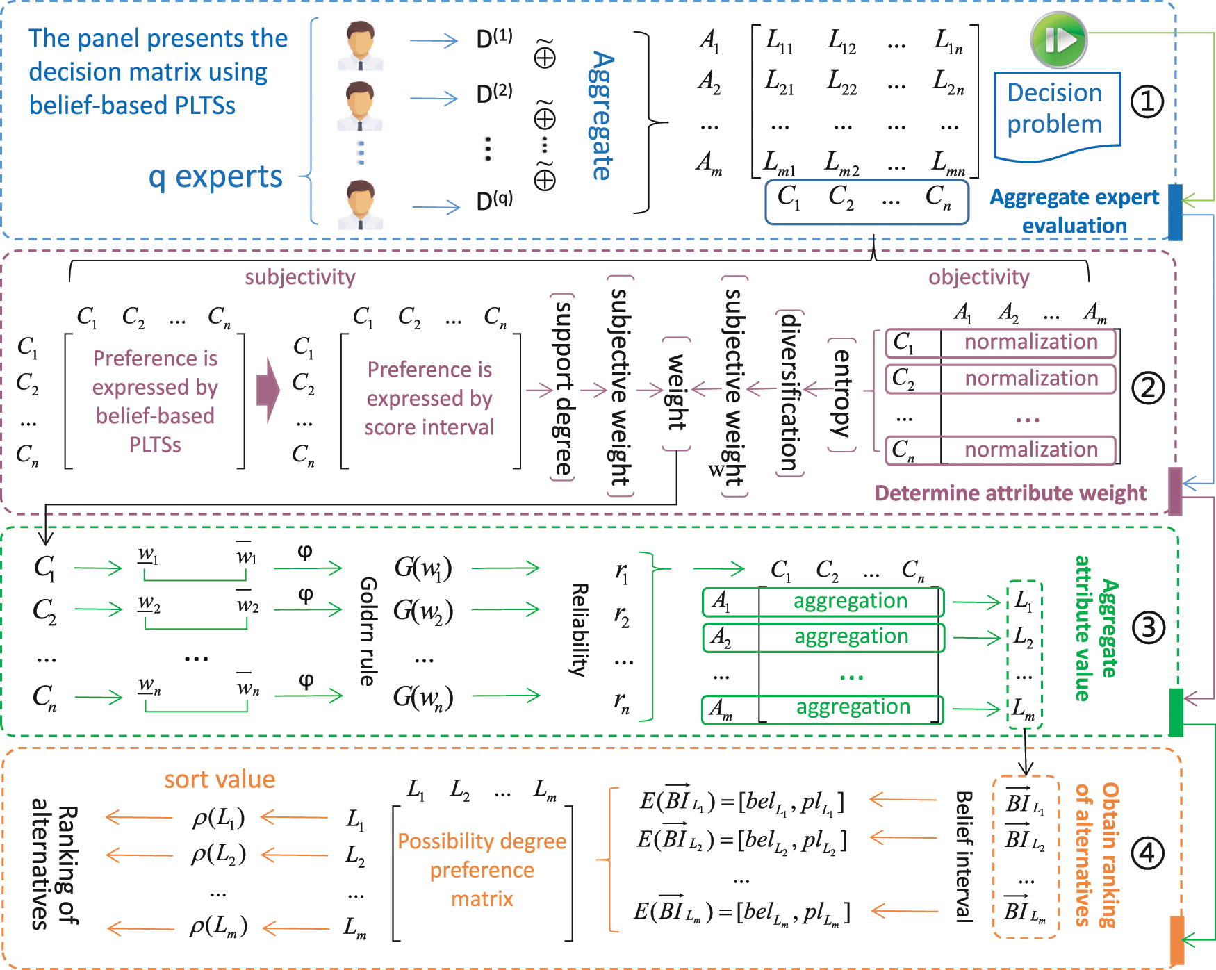
Figure 2: Emergency decision-making framework based on belief-based PLTSs
The emergency management bureau of municipality S (EMB-SM) is the agency responsible for the local government’s emergency management strategies. It coordinates and guides all districts in the city in responding to emergencies such as production safety, natural disasters, and comprehensive disaster prevention, mitigation and relief efforts. Citizen emergency education is an important step toward modernizing the emergency management system of municipality S. To this end, EMB-SM formulates three plans, namely, carrying out field exercises, developing emergency education apps, and disseminating emergency knowledge through propaganda manuals. In order to choose the most suitable of these three options, this section will demonstrate the effect of our proposed method based on a case study.
Based on the decision-making method in Section 4, the decision process of this case is shown as follows.
Three options (denoted as
To measure the level of suitability of emergency education plans, let the LTS be
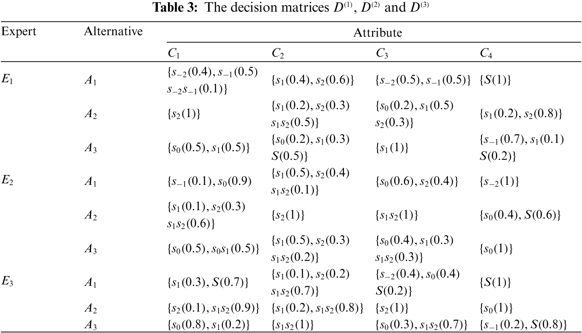
5.1.2 Aggregation of Decision Matrices from Different Experts
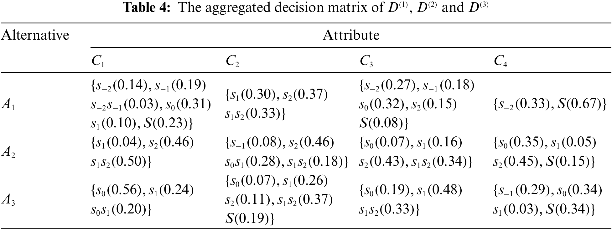
The decision matrices of
5.1.3 Determination of Attribute Weight
According to Section 4.3, the determination of attribute weight is divided into two parts: subjective and objective. We first determine the subjective weight of the attribute. The pair comparison between attributes
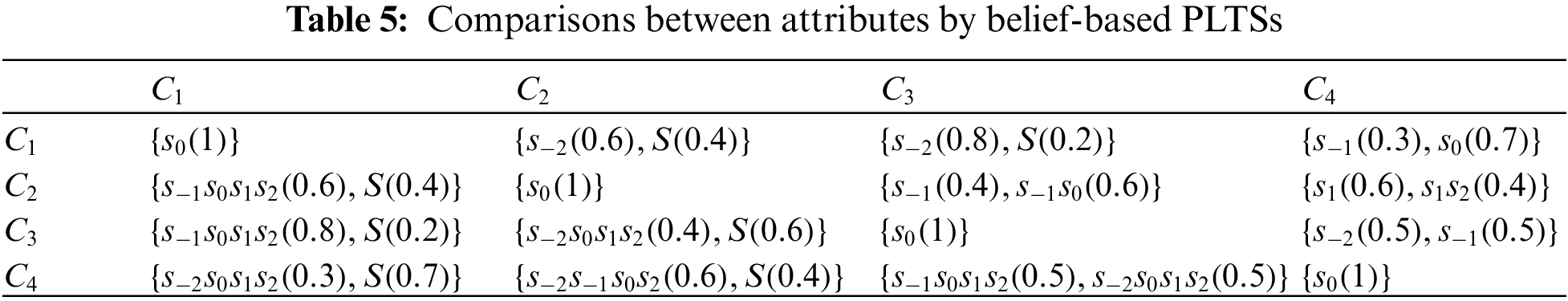
Based on Definition 3.13, the score of
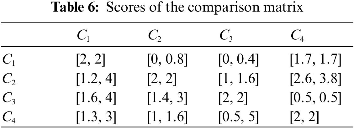
In what follows, the objective weight will be determined based on the interval entropy weight method. Based on the aggregated decision matrix in Table 4, the score of the evaluation of alternative
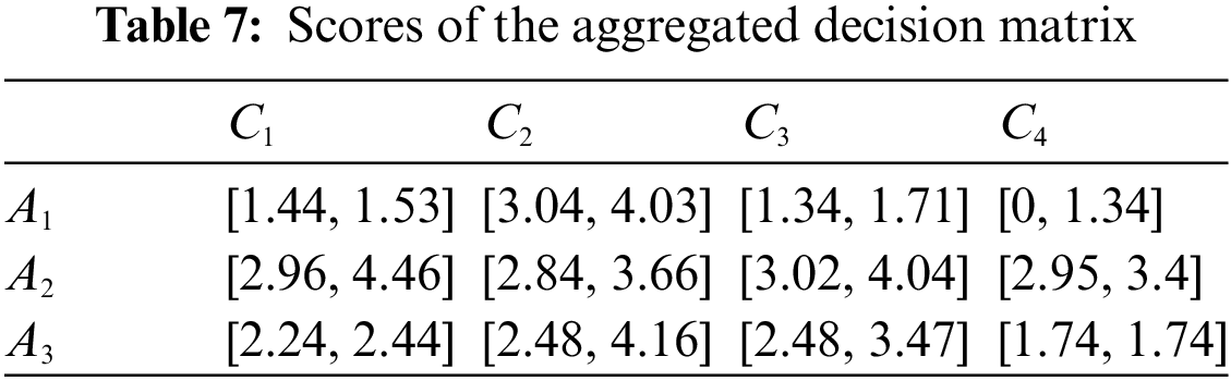
5.1.4 Aggregation of Attribute Information
Based on the attribute weights obtained and the decision matrix in Table 4, the evaluations of each alternative under different attributes can be aggregated by the aggregation operator in Section 3.2. First, the golden rule is used to transform the interval weight, without loss of generality, let
5.1.5 Calculation of the Ranking of Alternatives
According to the aggregated results, the final ranking of alternatives can be calculated by comparing the corresponding belief-based PLTSs. The sort value of
The decision method proposed in this study involves several parameters,
The parameter in the golden rule will be analyzed first. The function of the golden rule is to convert the interval weights into single values, where the parameter
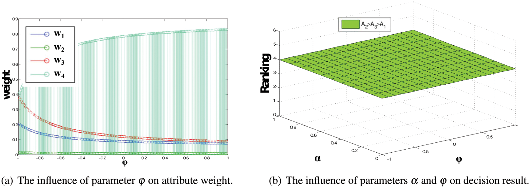
Figure 3: Sensitivity analysis of decision results to parameters
In addition, we analyze the influence of parameters
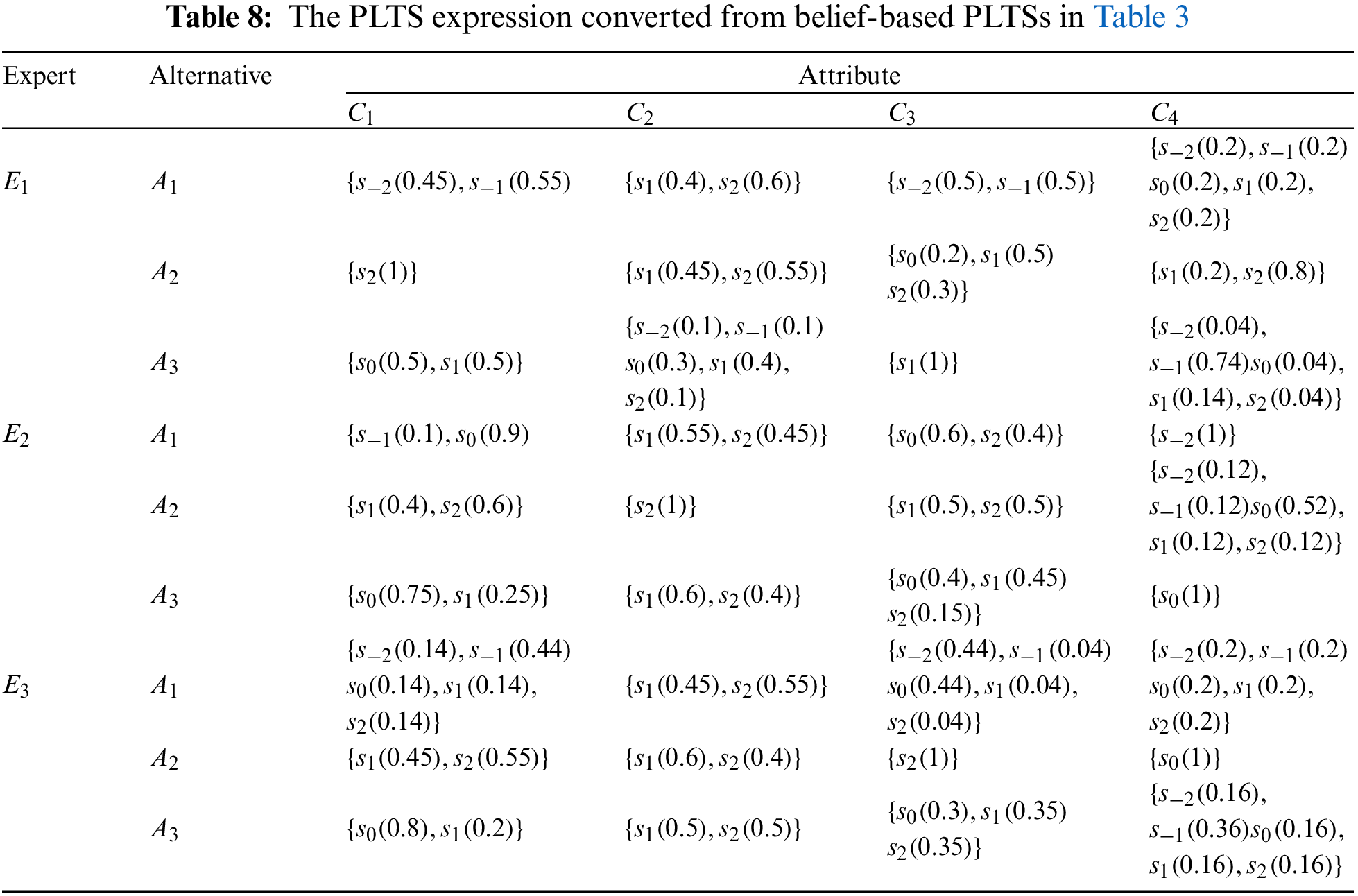
To further verify the effectiveness of the decision making method proposed in this paper, we conduct a group of comparative experiments and analyze the experimental results. We choose several decision methods with PLTS as the information expression to apply in the case in this paper. Since the data type in this study is belief-based PLTS, to adapt it to PLTS environment, we propose the following conversion method.
Definition 5.1. Let
where
Based on Definition 5.1, the belief-based PLTSs in Table 3 can be converted to PLTSs, as shown in Table 8. We will compare and analyze the different methods from the following aspects: aggregation operator, score function, attribute weight, applications, and ranking. The results of the comparison are shown in Table 9.
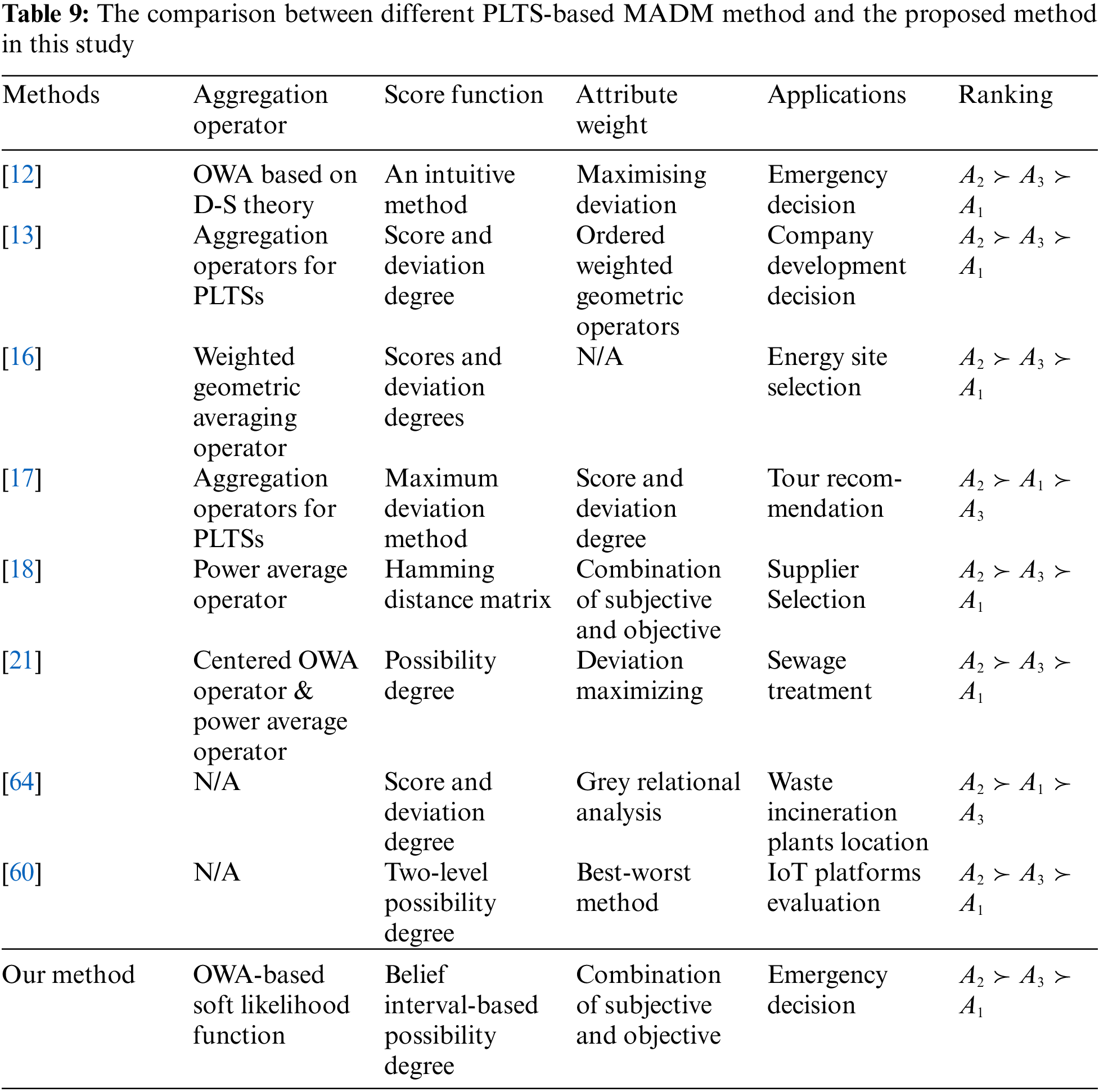
Through comparison, it can be seen that the advantages of the proposed method in this paper are as follows. First, the scope of expression of probabilistic linguistic information is extended, and the related operations that can be used in decision-making, including the aggregation operator and score functions, are proposed. Further, a decision-making framework is developed. In addition, in the determination of attribute weights, we take both subjective and objective aspects into consideration to avoid deviations caused by subjective weighting and make use of all decision information. Although other methods have their own unique characteristics, the superiority of the method presented in this study is quite obvious. From the ranking of the results, all methods suggest that option
6 Conclusions and Future Directions
Through a careful analysis of the relevant literature, we found that the traditional PLTS method has deficiencies in its expression of uncertain information. To overcome this limitation, we incorporated the belief function theory into PLTS to construct belief-based PLTS and proposed a corresponding decision analysis approach that is able to address the aforementioned deficiencies through methods such as probability allocation on multiple linguistic terms. We found that the OWA-based soft likelihood function can be employed to define the aggregation operator of belief-based PLTS, which has the advantage of being able to fully describe decision makers’ attitudes. In the actual decision-making environment, belief-based PLTSs are usually reliable, so we also put forward an aggregation operator that considers reliability. We found that the belief interval can express more complete linguistic information, so we defined a score function that uses the belief interval to compare different belief-based PLTSs. According to the results, a multi-attribute decision-making framework was constructed for linguistic environments that is suitable for emergency decisions and can potentially be applied to other areas. Finally, an example was given to demonstrate the usefulness and effectiveness of the proposed method.
In future research, we aim to further develop these theories and methods based on belief-based PLTS. First, we will study a variety of operations to further refine their mathematical forms. Second, more methods, such as the analytic network process and the best-worst method, will be used to determine attribute weights in the decision-making framework. Third, the decision problem presented by the heterogeneous attributes of the belief-based PLTS environment will be further studied. Finally, attribute interactivity should be taken into account in future research.
Funding Statement: The work is partially supported by National Social Science Foundation of China (Grant No. 17ZDA030).
Conflicts of Interest: The authors declare that they have no conflicts of interest to report regarding the present study.
References
1. Xu, X., Wang, L., Chen, X., Liu, B. (2019). Large group emergency decision-making method with linguistic risk appetites based on criteria mining. Knowledge-Based Systems, 182, 104849. DOI 10.1016/j.knosys.2019.07.020. [Google Scholar] [CrossRef]
2. Hao, Z., Xu, Z., Zhao, H., Fujita, H. (2017). A dynamic weight determination approach based on the intuitionistic fuzzy Bayesian network and its application to emergency decision making. IEEE Transactions on Fuzzy Systems, 26(4), 1893–1907. DOI 10.1109/TFUZZ.91. [Google Scholar] [CrossRef]
3. Karanci, A. N., Aksit, B., Dirik, G. (2005). Impact of a community disaster awareness training program in Turkey: Does it influence hazard-related cognitions and preparedness behaviors. Social Behavior and Personality: An International Journal, 33(3), 243–258. DOI 10.2224/sbp.2005.33.3.243. [Google Scholar] [CrossRef]
4. Tsai, M. H., Chang, Y. L., Shiau, J. S., Wang, S. M. (2020). Exploring the effects of a serious game-based learning package for disaster prevention education: The case of battle of flooding protection. International Journal of Disaster Risk Reduction, 43, 101393. DOI 10.1016/j.ijdrr.2019.101393. [Google Scholar] [CrossRef]
5. Sun, B., Qi, C., Ma, W., Wang, T., Zhang, L. et al. (2020). Variable precision diversified attribute multigranulation fuzzy rough set-based multi-attribute group decision making problems. Computers & Industrial Engineering, 142, 106331. DOI 10.1016/j.cie.2020.106331. [Google Scholar] [CrossRef]
6. Xu, X., Zhang, Q., Chen, X. (2020). Consensus-based non-cooperative behaviors management in large-group emergency decision-making considering experts’ trust relations and preference risks. Knowledge-Based Systems, 190, 105108. DOI 10.1016/j.knosys.2019.105108. [Google Scholar] [CrossRef]
7. Zeng, S., Chen, S. M., Fan, K. Y. (2020). Interval-valued intuitionistic fuzzy multiple attribute decision making based on nonlinear programming methodology and topsis method. Information Sciences, 506, 424–442. DOI 10.1016/j.ins.2019.08.027. [Google Scholar] [CrossRef]
8. Ding, W., Wang, J., Wang, J. (2020). Multigranulation consensus fuzzy-rough based attribute reduction. Knowledge-Based Systems, 105945. DOI 10.1016/j.knosys.2020.105945. [Google Scholar] [CrossRef]
9. Zavadskas, E. K., Bausys, R., Lescauskiene, I., Usovaite, A. (2021). Multimoora under interval-valued neutrosophic sets as the basis for the quantitative heuristic evaluation methodology hebin. Mathematics, 9(1), 66. DOI 10.3390/math9010066. [Google Scholar] [CrossRef]
10. Meng, F., Chen, S. M., Tang, J. (2020). Group decision making based on acceptable multiplicative consistency of hesitant fuzzy preference relations. Information Sciences, 524, 77–96. DOI 10.1016/j.ins.2020.03.037. [Google Scholar] [CrossRef]
11. Garg, H. (2020). Linguistic interval-valued pythagorean fuzzy sets and their application to multiple attribute group decision-making process. Cognitive Computation, 12(6), 1313–1337. DOI 10.1007/s12559-020-09750-4. [Google Scholar] [CrossRef]
12. Li, P., Wei, C. (2019). An emergency decision-making method based on ds evidence theory for probabilistic linguistic term sets. International Journal of Disaster Risk Reduction, 37, 101178. DOI 10.1016/j.ijdrr.2019.101178. [Google Scholar] [CrossRef]
13. Pang, Q., Wang, H., Xu, Z. (2016). Probabilistic linguistic term sets in multi-attribute group decision making. Information Sciences, 369, 128–143. DOI 10.1016/j.ins.2016.06.021. [Google Scholar] [CrossRef]
14. Liao, H., Wu, X. (2020). DNMA: A double normalization-based multiple aggregation method for multi-expert multi-criteria decision making. Omega, 94, 102058. DOI 10.1016/j.omega.2019.04.001. [Google Scholar] [CrossRef]
15. Jiang, L., Liao, H. (2020). Mixed fuzzy least absolute regression analysis with quantitative and probabilistic linguistic information. Fuzzy Sets and Systems, 387, 35–48. DOI 10.1016/j.fss.2019.03.004. [Google Scholar] [CrossRef]
16. Nie, R. X., Wang, J. Q. (2020). Prospect theory-based consistency recovery strategies with multiplicative probabilistic linguistic preference relations in managing group decision making. Arabian Journal for Science and Engineering, 45(3), 2113–2130. DOI 10.1007/s13369-019-04053-9. [Google Scholar] [CrossRef]
17. Wang, X., Wang, J., Zhang, H. (2019). Distance-based multicriteria group decision-making approach with probabilistic linguistic term sets. Expert Systems, 36(2), e12352. DOI 10.1111/exsy.12352. [Google Scholar] [CrossRef]
18. Wei, G., Wei, C., Wu, J., Wang, H. (2019). Supplier selection of medical consumption products with a probabilistic linguistic mabac method. International Journal of Environmental Research and Public Health, 16(24), 5082. DOI 10.3390/ijerph16245082. [Google Scholar] [CrossRef]
19. Li, B., Zhang, Y., Xu, Z. (2020). The medical treatment service matching based on the probabilistic linguistic term sets with unknown attribute weights. International Journal of Fuzzy Systems, 22, 1487–1505. DOI 10.1007/s40815-020-00844-7. [Google Scholar] [CrossRef]
20. Liang, D., Dai, Z., Wang, M., Li, J. (2020). Web celebrity shop assessment and improvement based on online review with probabilistic linguistic term sets by using sentiment analysis and fuzzy cognitive map. Fuzzy Optimization and Decision Making, 19, 561–586. DOI 10.1007/s10700-020-09327-8. [Google Scholar] [CrossRef]
21. Feng, X., Zhang, Q., Jin, L. (2019). Aggregation of pragmatic operators to support probabilistic linguistic multi-criteria group decision-making problems. Soft Computing, 24, 7735–7755. [Google Scholar]
22. Xie, W., Xu, Z., Ren, Z., Herrera-Viedma, E. (2020). A new multi-criteria decision model based on incomplete dual probabilistic linguistic preference relations. Applied Soft Computing, 106237. DOI 10.1016/j.asoc.2020.106237. [Google Scholar] [CrossRef]
23. Yang, J. B., Wang, Y. M., Xu, D. L., Chin, K. S. (2006). The evidential reasoning approach for mada under both probabilistic and fuzzy uncertainties. European Journal of Operational Research, 171(1), 309–343. DOI 10.1016/j.ejor.2004.09.017. [Google Scholar] [CrossRef]
24. Fang, R., Liao, H., Yang, J. B., Xu, D. L. (2021). Generalised probabilistic linguistic evidential reasoning approach for multi-criteria decision-making under uncertainty. Journal of the Operational Research Society, 72(1), 130–144. DOI 10.1080/01605682.2019.1654415. [Google Scholar] [CrossRef]
25. Lin, M., Xu, Z., Zhai, Y., Yao, Z. (2017). Multi-attribute group decision-making under probabilistic uncertain linguistic environment. Journal of the Operational Research Society, 68, 1–15. [Google Scholar]
26. Mi, X., Liao, H., Wu, X., Xu, Z. (2020). Probabilistic linguistic information fusion: A survey on aggregation operators in terms of principles, definitions, classifications, applications, and challenges. International Journal of Intelligent Systems, 35(3), 529–556. DOI 10.1002/int.22216. [Google Scholar] [CrossRef]
27. Liao, H., Mi, X., Xu, Z. (2020). A survey of decision-making methods with probabilistic linguistic information: Bibliometrics, preliminaries, methodologies, applications and future directions. Fuzzy Optimization and Decision Making, 19(1), 81–134. DOI 10.1007/s10700-019-09309-5. [Google Scholar] [CrossRef]
28. Fei, L., Feng, Y. (2021). Modeling interactive multiattribute decision-making via probabilistic linguistic term set extended by Dempster–Shafer theory. International Journal of Fuzzy Systems, 23(2), 599–613. DOI 10.1007/s40815-020-01019-0. [Google Scholar] [CrossRef]
29. Dempster, A. P. (1967). Upper and lower probabilities induced by a multivalued mapping. Annals of Mathematics and Statistics, 38(2), 325–339. DOI 10.1214/aoms/1177698950. [Google Scholar] [CrossRef]
30. Shafer, G. (1976). A mathematical theory of evidence. Princeton: Princeton University Press. [Google Scholar]
31. Wu, X., Liao, H., Zavadskas, E. K., Antuchevičienė, J. (2022). A probabilistic linguistic vikor method to solve mcdm problems with inconsistent criteria for different alternatives. Technological and Economic Development of Economy, 28(2), 559–580. DOI 10.3846/tede.2022.16634. [Google Scholar] [CrossRef]
32. Deng, Y. (2020). Information volume of mass function. International Journal of Computers, Communications & Control, 15(6), 3983. DOI 10.15837/ijccc.2020.6.3983. [Google Scholar] [CrossRef]
33. Xiao, F. (2021). CEQD: A complex mass function to predict interference effects. IEEE Transactions on Cybernetics, 52(8), 7402–7414. [Google Scholar]
34. Deng, Y. (2020). Uncertainty measure in evidence theory. Science China Information Sciences, 63(11), 1–19. DOI 10.1007/s11432-020-3006-9. [Google Scholar] [CrossRef]
35. Xiao, F. (2021). CaFtR: A fuzzy complex event processing method. International Journal of Fuzzy Systems, 1–14. DOI 10.1007/s40815–021–01118–6. [Google Scholar] [CrossRef]
36. Deng, X., Jiang, W. (2020). On the negation of a Dempster–Shafer belief structure based on maximum uncertainty allocation. Information Sciences, 516, 346–352. DOI 10.1016/j.ins.2019.12.080. [Google Scholar] [CrossRef]
37. Zhang, H., Jiang, W., Deng, X. (2020). Data-driven multi-attribute decision-making by combining probability distributions based on compatibility and entropy. Applied Intelligence, 50(11), 4081–4093. DOI 10.1007/s10489-020-01738-9. [Google Scholar] [CrossRef]
38. Mahmood, T., Ali, Z. (2020). Aggregation operators and vikor method based on complex q-rung orthopair uncertain linguistic informations and their applications in multi-attribute decision making. Computational and Applied Mathematics, 39(4), 1–44. DOI 10.1007/s40314-020-01332-2. [Google Scholar] [CrossRef]
39. Xu, Z. (2005). Deviation measures of linguistic preference relations in group decision making. Omega, 33(3), 249–254. DOI 10.1016/j.omega.2004.04.008. [Google Scholar] [CrossRef]
40. Deng, Y. (2022). Random permutation set. International Journal of Computers Communications & Control, 17(1), 4542. DOI 10.15837/ijccc.2022.1.4542. [Google Scholar] [CrossRef]
41. Ding, W., Lin, C. T., Liew, A. W. C., Triguero, I., Luo, W. (2020). Current trends of granular data mining for biomedical data analysis. Information Sciences, 510, 341–343. DOI 10.1016/j.ins.2019.10.002. [Google Scholar] [CrossRef]
42. Fang, R., Liao, H., Mardani, A. (2022). How to aggregate uncertain and incomplete cognitive evaluation information in lung cancer treatment plan selection? A method based on dempster-shafer theory. Information Sciences, 603, 222–243. DOI 10.1016/j.ins.2022.04.060. [Google Scholar] [CrossRef]
43. Qiang, C., Deng, Y., Cheong, K. H. (2022). Information fractal dimension of mass function. Fractals, 30(6), 2250110. DOI 10.1142/S0218348X22501109. [Google Scholar] [CrossRef]
44. Zhou, Q., Deng, Y., Pedrycz, W. (2022). Information dimension of Galton board. Fractals, 30(4), 2250079. DOI 10.1142/S0218348X22500797. [Google Scholar] [CrossRef]
45. Liu, R., Fei, L., Mi, J. (2022). An evidential multimoora approach to assessing disaster risk reduction education strategies under a heterogeneous linguistic environment. International Journal of Disaster Risk Reduction, 78, 103114. DOI 10.1016/j.ijdrr.2022.103114. [Google Scholar] [CrossRef]
46. Denoeux, T., Shenoy, P. P. (2020). An interval-valued utility theory for decision making with dempster-shafer belief functions. International Journal of Approximate Reasoning, 124, 194–216. DOI 10.1016/j.ijar.2020.06.008. [Google Scholar] [CrossRef]
47. Deng, Z., Wang, J. (2020). A novel decision probability transformation method based on belief interval. Knowledge-Based Systems, 208, 106427. DOI 10.1016/j.knosys.2020.106427. [Google Scholar] [CrossRef]
48. Yager, R. R. (1988). On ordered weighted averaging aggregation operators in multicriteria decisionmaking. IEEE Transactions on Systems, Man, and Cybernetics, 18(1), 183–190. DOI 10.1109/21.87068. [Google Scholar] [CrossRef]
49. Jin, L., Mesiar, R., Kalina, M., Yager, R. R. (2020). Canonical form of ordered weighted averaging operators. Annals of Operations Research, 295(2), 605–631. DOI 10.1007/s10479-020-03802-6. [Google Scholar] [CrossRef]
50. Jin, L., Mesiar, R., Yager, R. (2020). Parameterized preference aggregation operators with improved adjustability. International Journal of General Systems, 49(8), 843–855. DOI 10.1080/03081079.2020.1786822. [Google Scholar] [CrossRef]
51. Yager, R. R. (1996). Quantifier guided aggregation using owa operators. International Journal of Intelligent Systems, 11(1), 49–73. DOI 10.1002/(SICI)1098-111X(199601)11:1<49::AID-INT3>3.0.CO;2-Z. [Google Scholar] [CrossRef]
52. Klir, G. J., Wierman, M. J. (2013). Uncertainty-based information: Elements of generalized information theory, vol. 15. New York: Physica. [Google Scholar]
53. Yager, R. R., Elmore, P., Petry, F. (2017). Soft likelihood functions in combining evidence. Information Fusion, 36, 185–190. DOI 10.1016/j.inffus.2016.11.013. [Google Scholar] [CrossRef]
54. Zhu, R., Liu, Q., Huang, C., Kang, B. (2022). Z-ACM: An approximate calculation method of z-numbers for large data sets based on kernel density estimation and its application in decision-making. Information Sciences, 610, 440–471. DOI 10.1016/j.ins.2022.07.171. [Google Scholar] [CrossRef]
55. Flores-Sosa, M., Avilés-Ochoa, E., Merigó, J. M., Yager, R. R. (2021). Volatility garch models with the ordered weighted average (OWA) operators. Information Sciences, 565, 46–61. DOI 10.1016/j.ins.2021.02.051. [Google Scholar] [CrossRef]
56. Mi, X., Tian, Y., Kang, B. (2020). A modified soft-likelihood function based on powa operator. International Journal of Intelligent Systems, 35(5), 869–890. DOI 10.1002/int.22228. [Google Scholar] [CrossRef]
57. Fei, L., Wang, Y. (2022). An optimization model for rescuer assignments under an uncertain environment by using dempster-shafer theory. Knowledge-Based Systems, 109680. DOI 10.1016/j.knosys.2022.109680. [Google Scholar] [CrossRef]
58. Fei, L., Feng, Y. (2021). A dynamic framework of multi-attribute decision making under pythagorean fuzzy environment by using Dempster–Shafer theory. Engineering Applications of Artificial Intelligence, 101, 104213. DOI 10.1016/j.engappai.2021.104213. [Google Scholar] [CrossRef]
59. Xu, Z., Da, Q. (2003). Possibility degree method for ranking interval numbers and its application. Journal of Systems Engineering, 18(1), 67–70. [Google Scholar]
60. Lin, M., Huang, C., Xu, Z., Chen, R. (2020). Evaluating iot platforms using integrated probabilistic linguistic mcdm method. IEEE Internet of Things Journal, 7(11), 11195–11208. DOI 10.1109/JIoT.6488907. [Google Scholar] [CrossRef]
61. Yager, R. R. (2014). On the maximum entropy negation of a probability distribution. IEEE Transactions on Fuzzy Systems, 23(5), 1899–1902. DOI 10.1109/TFUZZ.2014.2374211. [Google Scholar] [CrossRef]
62. Fei, L. (2019). On interval-valued fuzzy decision-making using soft likelihood functions. International Journal of Intelligent Systems, 34(7), 1631–1652. DOI 10.1002/int.22110. [Google Scholar] [CrossRef]
63. Kraiger, K., Ford, J. K., Salas, E. (1993). Application of cognitive, skill-based, and affective theories of learning outcomes to new methods of training evaluation. Journal of Applied Psychology, 78(2), 311–328. DOI 10.1037/0021-9010.78.2.311. [Google Scholar] [CrossRef]
64. Lei, F., Wei, G., Lu, J., Wu, J., Wei, C. (2019). Gra method for probabilistic linguistic multiple attribute group decision making with incomplete weight information and its application to waste incineration plants location problem. International Journal of Computational Intelligence Systems, 12(2), 1547–1556. DOI 10.2991/ijcis.d.191203.002. [Google Scholar] [CrossRef]
Cite This Article
 Copyright © 2023 The Author(s). Published by Tech Science Press.
This work is licensed under a Creative Commons Attribution 4.0 International License , which permits unrestricted use, distribution, and reproduction in any medium, provided the original work is properly cited.
 Downloads
 Citation Tools