Importance of Three-Dimensional Piezoelectric Coupling Modeling in Quantitative Analysis of Piezoelectric Actuators

1  Introduction

Piezoelectric materials can serve as sensors based on the accumulation of electric charge in response to mechanical strain, called the direct piezoelectric effect (DPE) [1], or as actuators based on the change in size in response to an applied electric potential, called the inverse piezoelectric effect (IPE) [2]. Both sensor and actuator modes have been incorporated in intelligent structures [3]. Piezoelectric devices have become increasingly applied in vibration control [4,5], energy harvesting [6–8], and nano-aerial vehicles [9–11].

A typical simplified model of these devices is the thin cantilevered piezoelectric bimorph beam. Its electromechanical behavior has been extensively studied using a variety of theoretical approaches [8,12–14] using a closed-form solution under the Euler-Bernoulli beam assumption.

In general, the configuration of piezoelectric devices is more complicated in terms of geometry, material positioning, and electrode patterns. Numerical approaches are needed to simulate the electromechanical behavior of such systems [15,16]. Numerical studies often introduce simplified modeling such as order reduction of piezoelectric effects for electric circuit elements [17,18] and weakly coupled DPE and IPE [19,20]. Several algorithms for strongly coupled DPE and IPE have been compared with each other [21]. The partitioned method can be effectively used for a thin piezoelectric bimorph plate analysis [22]. Most recently, a partitioned method has been proposed for strongly coupled DPE, IPE, and fluid flow field or electric circuit [23,24].

The present study mainly focuses on thin cantilevered piezoelectric bimorph actuators and sensors. Previous studies used various simplified models for this configuration for both analytical and numerical approaches. However, a thin cantilevered piezoelectric bimorph sensor can have a complicated three-dimensional (3-D) distribution of the electric field in the thin piezoelectric continuum [25].

Similarly, for a thin cantilevered piezoelectric bimorph actuator, cases for which direct modeling of 3-D piezoelectric coupling is important must be determined. Many studies focus on the finite element modeling of adaptive structural elements, namely, solids, shells, plates and beams [15]. However, as long as we know, few studies have considered this task because of the complexity of 3-D piezoelectric coupling. Therefore, in the present study, coupling of the DPE and the IPE (i.e., piezoelectric coupling) and the 3-D IPE in a thin cantilevered piezoelectric bimorph actuator is systematically investigated as follows:

In Section 3, the bending of the beam with various piezoelectric coupling coefficients taken from actual materials is considered. Here, the theoretical solution, which considers the 1D IPE, the numerical weak coupling (NWC) solution, which considers the 3-D IPE, and the numerical strong coupling (NSC) solution, which considers both the 3-D IPE and the piezoelectric coupling effect (PCE), are compared with each other to illustrate the importance of the piezoelectric coupling modeling. In Section 4, the bending of the plate is considered. Here, first, the theoretical and NWC solutions are compared with each other to illustrate the importance of the 3-D IPE, and then they are compared with the NSC solution in order to illustrate how the combination of this two importance appears in the NSC solution. The results demonstrate that 3-D piezoelectric coupling modeling is important for quantitatively evaluating the electromechanical behavior of a thin cantilevered piezoelectric bimorph actuator.

2  Materials and Methods

2.1 Governing Equations for Piezoelectric Material and Finite Element Formulations

The electromechanical behavior of a piezoelectric material can be expressed as

σij,j+fi=0(1)

Di,i=0(2)

where σij, fi, and Di are the ij-th component of the mechanical stress tensor, the i-th component of the body force vector, and the i-th component of the electric displacement vector, respectively. Note that ‘, j’ denotes the differential with respect to the j-th coordinate. The constitutive equations for the linear piezoelectric effect can be written using a tensor representation of the stress-electric displacement form as

σij=CijklESkl−ekijEk(3)

Di=eiklSkl+εikSEk(4)

where Cijkl, Sij, eijk, Ei, and εij are the ijkl-th component of the elastic tensor, the ij-th component of the mechanical strain tensor, the ijk-th component of the piezoelectric constant tensor, the i-th component of the electric field vector, and the ij-th component of the dielectric constant tensor, respectively. The superscripts E and S indicate that the quantities are determined under constant electric and strain fields, respectively. Sij and Ei are respectively given as

Sij=(ui,j+uj,i)/2(5)

Ei=−φ,i(6)

where ui and φ are the i-th component of the mechanical displacement vector and the electric potential, respectively. The conditions imposed on the elementary and natural boundaries can be expressed as

ui=ui∗ on Γu(7)

φ=φ∗ on Γφ(8)

σijnj=fi∗ on Γσ(9)

Dini=q∗ on Γq(10)

where fi and q are the surface force and charge, respectively, the superscript * denotes that the quantities are prescribed, and ni is the i-th component of the unit vector outward normal to each boundary.

The weak forms of Eqs. (1) and (2) are obtained using the method of weighted residuals [26,27]. For arbitrary space-variable and virtual displacements δui, and virtual electric potential δφ, Eqs. (1) and (2) can be written in integral forms, which are respectively reduced using integration by parts and the divergence theorem to

−∫Ωσijδui,jdΩ+∫ΓσσijnjδuidΓ+∫ΩfiδuidΩ=0(11)

−∫ΩDiδφ,idΩ+∫ΓqDiniδφdΓ−∫ΩqδφdΩ=0(12)

Substituting Eq. (9) and the virtual strain δSij into Eq. (11) gives

−∫ΩσijδSijdΩ+∫ΓσfiδuidΓ+∫ΩfiδuidΩ=0(13)

Substituting Eq. (10) and the virtual electric field δEi into Eq. (12) gives

−∫ΩDiδφ,idΩ+∫ΓqDiniδφdΓ−∫ΩqδφdΩ=0(14)

By substituting the piezoelectric constitutive equations (Eqs. (3) and (4)) into the principle of virtual displacement equation (Eq. (13)) and the principle of virtual electric potential equation (Eq. (14)), respectively, the following set of equations is obtained after suitable rearrangement:

∫ΩCijklESklδSijdΩ−∫ΩekijEkδSijdΩ=∫Γσfi∗δuidΓ+∫ΩfiδuidΩ(15)

∫ΩeiklSklδEidΩ+∫ΩεikSEkδEidΩ=−∫Γqq∗δφdΓ(16)

Based on these equations, the spatially discretized equations of motion for linear piezoelectricity in the global coordinate system are derived as

Kuuu+Kuφφ=f(17)

KuφTu+Kφφφ=q(18)

where Kuu is the global mechanical stiffness matrix, Kuφ is the global piezoelectric stiffness matrix, Kφφ is the global dielectric stiffness matrix, u is the nodal global vector for the mechanical displacement, φ is the nodal global vector for the electric potential, f is the global equivalent vector for the mechanical external force, q is the global equivalent vector for the external surface charge, and the superscript T denotes the transpose of the matrix. In this study, Eqs. (17) and (18) are respectively referred to as the IPE and DPE equations.

Piezoelectric ceramics such as lead zirconate titanate (PZT), lithium niobate (LiNbO3), and lithium tantalate (LiTaO3) are the most commonly used piezoelectric materials. In general, these poled piezoceramics are transversely isotropic materials [8]. Here, the plane of isotropy is defined as the xy-plane, and thus the piezoelectric material exhibits symmetry about the z-axis, which is the poling axis of the material. The piezoelectric constitutive equations (Eqs. (3) and (4)) can be given in matrix form as

[σD]=[CEeTeεS][SE](19)

where C is the elastic constitutive matrix, e is the piezoelectric stress coefficient matrix, and ε is the dielectric permittivity matrix. An alternative form of C is the elastic compliance matrix S, which is defined as S = C−1. The vectors for the stress σ, strain S, electric displacement D, and electric field E are respectively defined as

σ=[σ11σ22σ33σ23σ13σ12]T(20)

S=[S11S22S332S232S132S12]T(21)

D=[D1D2D3]T(22)

E=[E1E2E3]T(23)

For PZT, which is used in this study, the expanded forms of CE, e, and εS can be respectively given as

CE=[C11EC12EC13E000C11EC13E000C33E000C44E00Sym.C44E0C66E](24)

e=[0000e150000e1500e31e31e33000](25)

εS=[ε11S000ε11S000ε33S](26)

C66E is given as C66E=(C11E−C12E)/2 and e is given using the piezoelectric strain coefficient matrix d as

e=dCE(27)

2.2 Strong and Weak Coupling Methods

The focus of this study is the importance of 3-D piezoelectric coupling in the thin cantilevered piezoelectric bimorph actuator. For this purpose, strong and weak coupling methods are developed. These methods were implemented as in-house computer programs.

Various coupling modeling (monolithic, partitioned, or splitting; strong or weak; implicit or explicit) can be seen in previous literatures. The coupling methods can be roughly divided into two approaches. One is the monolithic approach, and the other is the partitioned approach. The monolithic approach gives strong coupling methods, while the partitioned approach gives both strong and weak coupling methods.

The performance comparison of the several coupling methods including the strong coupling method used here, the monolithic method, and the explicit method was conducted in our previous study for the purpose of illustrating the relative merit and demerit of these methods [21]. Sections 3 and 4 include the basic validation of two coupling method, which was conducted using the theoretical solution.

2.2.1 Strong Coupling Method Using Block Gauss-Seidel Algorithm

We consider a method based on the block Gauss-Seidel (BGS) algorithm, which is a partitioned iterative coupling algorithm. If convergence is achieved in the solution procedure of this method, the solution will exactly satisfy the coupled equation system. Such a method is said to be strongly coupled [28]. Applying the BGS algorithm to Eqs. (17) and (18) yields the following reduced equations:

Kφφφ(i)=q−KuφTu(i−1)(28)

Kuuu(i)=f−Kuφφ(i)(29)

For a given i, the potential φ(i) is obtained by solving the DPE Eq. (28) using u(i−1), which is obtained in the previous iteration i−1, and then the current displacement u(i) is obtained by solving the IPE equation (Eq. (29)) using the current potential φ(i). This procedure is repeated for i = 1, 2, …, until convergence is achieved. The initial displacement u(0) is set to 0. The convergence criterion for terminating an iteration is

|(U(i)−U(i−1))/U(i)|<10−6(30)

where U(i) is the maximum bending displacement at the i-th BGS iteration.

2.2.2 Weak Coupling Method

We denote φ in the piezoelectric continuum subjected to an external voltage with no coupling effect as φ∗. This predictor can be obtained by solving the DPE Eq. (18) with u = 0 as

Kφφφ∗=q(31)

Then, the displacement u can be obtained by solving the IPE equation (Eq. (19)) using the predictor φ∗ as

Kuuu=f−Kuφφ∗(32)

This procedure results in a weak coupling method because it ignores the DPE, and the solution does not exactly satisfy the coupled equation system (Eqs. (17) and (18)).

2.3 Piezoelectric Actuator Model and Theoretical Solution

As shown in Fig. 1, the cantilevered symmetric and uniform bimorph configuration is considered as the piezoelectric actuator model. In the composite structure, the piezoceramic and electrode layers are assumed to be perfectly bonded to each other. The outer two layers are piezoceramics poled in the thickness direction and the bracketed layer is a metallic substructure, which serves as an electrode. The electrodes cover the opposite transverse faces of the piezoceramic layers. All electrodes are assumed to be very thin compared to the overall thickness such that their contribution to the overall stiffness is negligible. Hence, only the piezoceramic layers are assumed to be present.

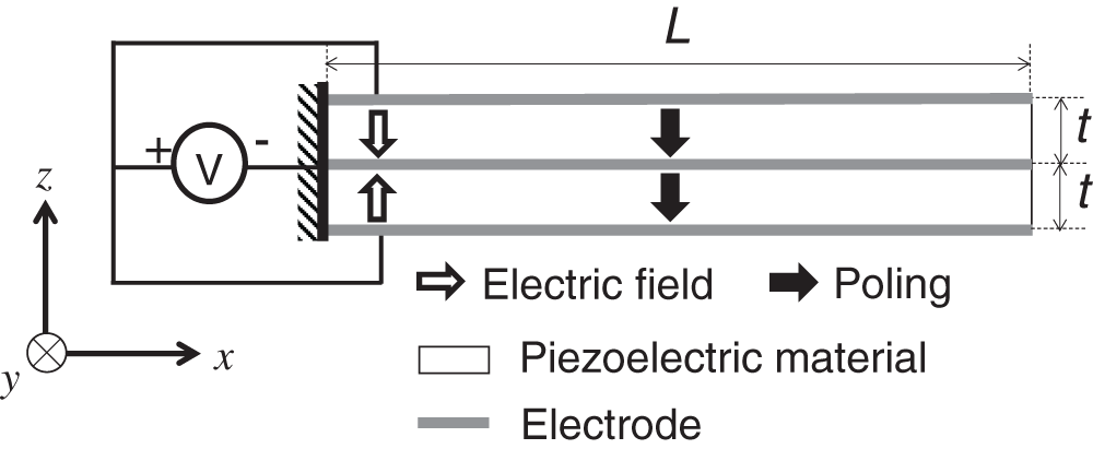
Figure 1: Piezoelectric actuator model with the cantilevered symmetric and uniform bimorph configuration subjected to an external voltage

As shown in Fig. 1, the length, width, and thickness directions of the bimorph actuator are assigned as the x-, y-, and z-directions, respectively. The directional parameters for the piezoelectric constants are indicated by the subscripts 1, 2, and 3, which correspond to the x-, y-, and z-directions, respectively. The electrodes that cover the top and bottom faces and the interface of the piezoceramic layers are assumed to be perfectly conductive.

The piezoceramic layers are poled in the same direction, namely the thickness direction or the z-direction. This configuration represents the parallel connection of the piezoceramic layers. As shown in Fig. 1, this configuration is subjected to an external voltage that produces an electric field across each individual layer with opposite polarity. The induced electric forces in the upper and lower half thicknesses cancel each other. The upper and lower piezoelectric layers contract and expand, respectively, resulting in pure bending in the upward direction.

It should be noted here that the solution procedure for the weak coupling method in the previous section is equivalent to that used to obtain the following closed-form solution of the tip bending displacement of the cantilevered bimorph beam [29]:

δ=(3/4)d31(L/t)2V(33)

where d31 is the piezoelectric strain constant, L is the length of the bimorph, t is the thickness of each piezoelectric layer, and V is the external voltage applied to the bimorph. This solution is given under the Euler-Bernoulli beam assumption. Furthermore, the one-way coupling of the piezoelectricity is assumed [8,29]. That is, it is assumed that the electric field applied across each individual layer with opposite polarity is determined by the external voltage only; that is, it is independent of the DPE caused by the deformation. Hence, the instantaneous electric fields induced in the piezoceramic layers are assumed to be uniform throughout the length of the beam.

3  Importance of Piezoelectric Coupling Modeling

In this section, the effect of piezoelectric coupling on the analysis results is investigated. A thin cantilevered piezoelectric bimorph actuator is analyzed using the theoretical solution, the numerical weak coupling solution, and the numerical strong coupling solution. The ratio of the length to the sectional dimension is 100, which is large enough to sufficiently satisfy the Euler-Bernoulli beam assumption. Hence, the differences in the solutions are caused only by the differences in the coupling models. The weak coupling model, which considers only the IPE, is used for the theoretical and numerical weak coupling formulations, and the strong coupling model, which considers both the DPE and the IPE (i.e., piezoelectric coupling), is used for the numerical strong coupling formulation.

3.1 Problem Setup

The piezoelectric actuator model presented in Section 2.3 is used here. The piezoelectric bimorph in Fig. 1 has a length of L = 100 mm, a layer thickness of t = 0.5 mm, and a width of w = 1 mm. The ratio of the bimorph length to the sectional dimension is sufficiently large. The material properties of PZT used in this section are summarized in Table 1. The external voltage applied to the bimorph is 1 V. The section of the one end is fixed in the length direction, one edge of this section along the thickness direction is fixed in the width direction, and one edge of this section along the width direction is fixed in the thickness direction.

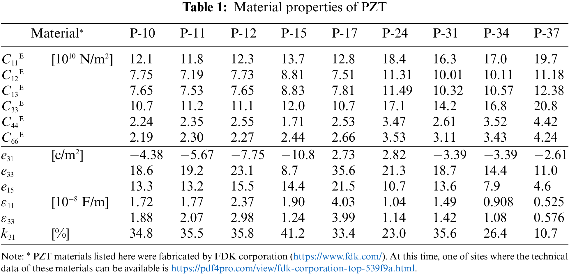
The typical finite element mesh is shown in Fig. 2, where 20-node hexahedral elements are used. As shown in this figure, each mesh is uniformly divided in all directions. The finer meshes are considered as follows: (1) the finer mesh-1 (Fig. 2), where 100, 4, and 1 element divisions are used along the length (x-axis), thickness (z-axis), and width (y-axis) directions, respectively, and (2) the finer mesh-2, where 100, 4, and 2 element divisions are used along the length, thickness, and width directions, respectively. The coarser meshes are considered as follows: (1) the coarser mesh-1, where 50, 4, and 1 element divisions are used along the length, thickness, and width directions, respectively, and (2) the coarser mesh-2, where 100, 2, and 1 element divisions are used along the length, thickness, and width directions, respectively.

Figure 2: Finite element mesh for piezoelectric actuator model, of which boundary conditions are illustrated in Fig. 1

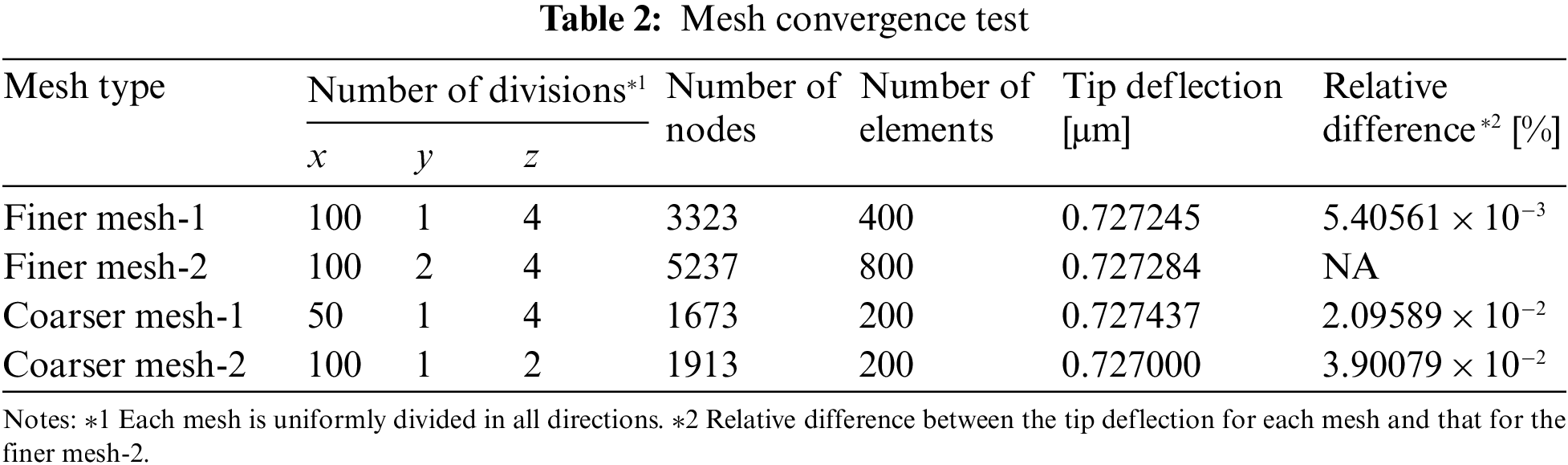
In order to check the mesh convergence, the bimorph with the P-15 material in Table 1 is analyzed using the numerical strong coupling solution. The results are summarized in Table 2. As shown in this table, the relative difference among the tip deflections is sufficiently small. Hence, in the following section, the finer mesh-1 is used.

3.2 Results and Discussion

The strong and weak coupling methods are used to analyze the problem described in Section 3.1. The relative differences in their solutions for the tip displacement in the z-direction compared to the corresponding theoretical solution are investigated for various PZT materials. The electromechanical coupling factor kij, which indicates the effectiveness of a piezoelectric material at converting between electrical energy and mechanical energy [30], is used to measure the coupling strength between the DPE and the IPE. For kij, the subscript i denotes the polarized direction or the direction along which the electrodes are applied (i.e., the direction of the electric field), and the subscript j denotes the direction perpendicular to the polarized direction or the direction along which the mechanical energy is developed. Hence, k31 is used here, which is given as [31]

k31=d31/ε33S11E(34)

where d31 is the piezoelectric strain constant, ε33 is the dielectric constant, and SE11 is the elastic compliance constant. The values of k31 for the PZT materials are summarized in Table 1.

Fig. 3 shows the relationship between k31 and the relative difference between the numerical solution and the theoretical solution for the tip displacement. The relative difference between the numerical weak coupling solution and the theoretical solution (white circles) ranges from + 0.028% to + 0.053% and is almost independent of k31. The Euler-Bernoulli beam assumption is sufficiently satisfied for the present cantilever and the same weak coupling model for piezoelectricity is used for the theoretical formulation in Eq. (33) and the numerical weak coupling formulation in Section 2.2. Hence, the numerical weak coupling solution is very close to the theoretical solution, as shown in Fig. 3. In contrast, the relative difference between the numerical strong coupling solution and the theoretical solution (black circles) shows an almost linear dependence on k31. For the tested materials shown in Table 1, a smaller k31 value led to a smaller relative difference between the solutions. For example, the relative difference is −0.68% for k31 = 10.7% (the lowest value of k31 for the tested materials, i.e., PZT material P-37 in Table 1) and increases almost linearly up to −8.32% for k31 = 41.2% (the highest value of k31 for the tested materials, i.e., PZT material P-15 in Table 1). As shown, the difference between the strong and weak coupling solutions will be significant for actual piezoelectric materials with high conversion effectiveness between electrical energy and mechanical energy. In such cases, the DPE and the IPE need to be solved simultaneously.

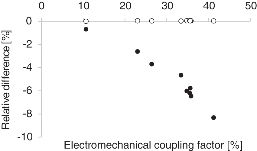
Figure 3: Relationship between electromechanical coupling factor and relative difference of strongly (black circles) and weakly (white circles) coupled numerical solutions compared to the theoretical solution

To provide more direct evidence of the importance of the DPE, the electric potential distributions in the thin piezoelectric continuum at the free and fixed ends are plotted along the thickness direction in Figs. 4A and 4B, respectively. As shown, the electric potential for k31 = 10.7% is distributed linearly along the thickness direction, as assumed in the theoretical formulation. In contrast, the electric potential for k31 = 41.2% (PZT material P-15 in Table 1) is distributed quadratically along the thickness direction because the electric potential at each point except on the electrodes is reduced by the DPE to be lower than that of the linear distribution while the electric potential on each electrode is prescribed to be 0 or 1 V.

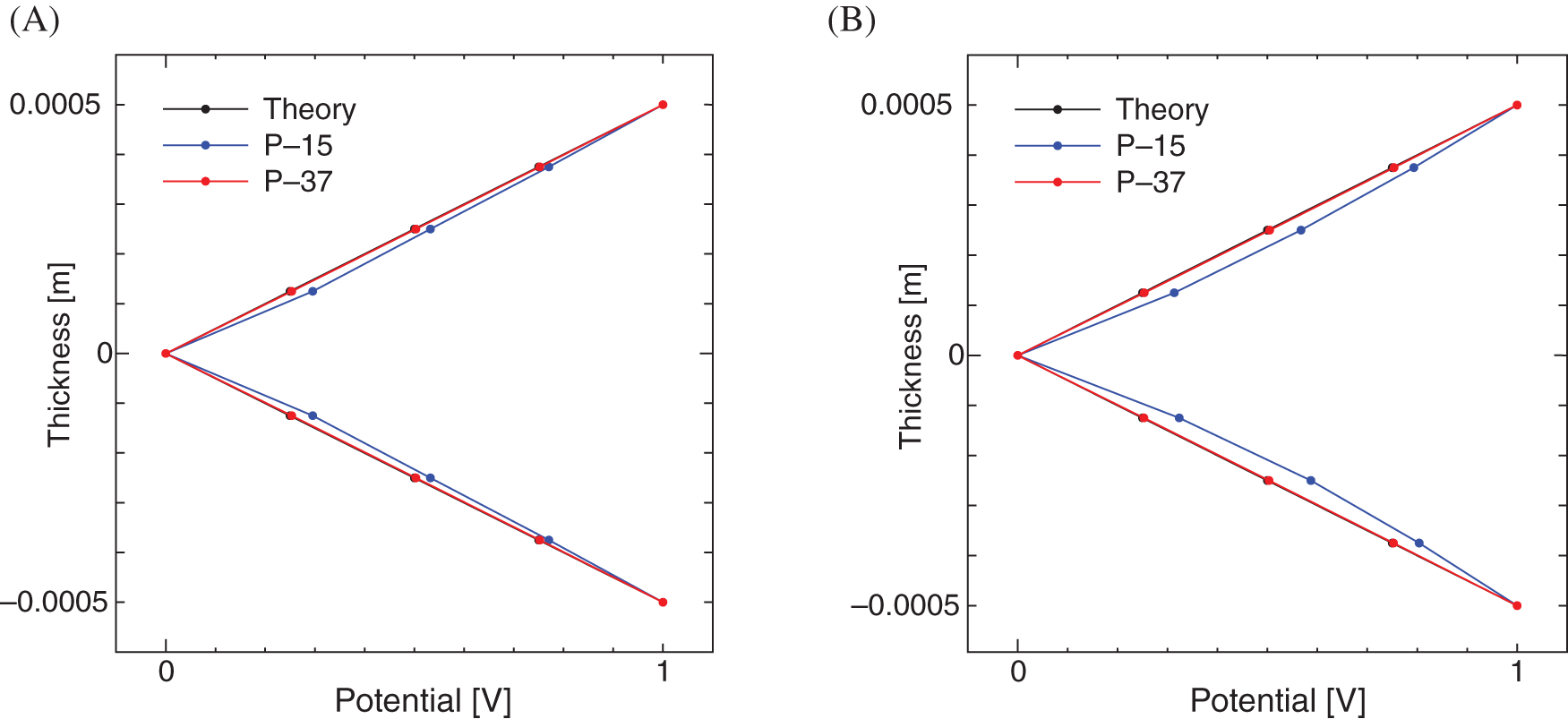
Figure 4: Potential distributions along thickness direction for thin piezoelectric continuum at free end (A) and fixed end (B). The black, blue, and red curves respectively show the theoretical solution, the numerical solution for the PZT material P-15 in Table 1, and the numerical solution for the PZT material P-15 in Table 1

4  Importance of Three-Dimensional Piezoelectric Modeling

In this section, the importance of the 3-D piezoelectric effect in the analysis is investigated. First, a thin cantilevered piezoelectric bimorph actuator is analyzed using the theoretical solution and the numerical weak coupling solution. This structure is sufficiently thin but wider than the beam used in the previous section. The dimensions used here are based on an actual actuator. Roller support is used at the fixed end, as shown in Fig. 5. In the pure elastic analysis for this setup, the theoretical solution well agrees with the 3-D finite element solution. Hence, the only difference between the theoretical solution and the numerical weak coupling solution in the piezoelectric analysis for this setup is that the numerical weak coupling solution considers the IPE in the x-, y-, and z-directions, whereas the theoretical solution given by Eq. (33) considers only that in the x-direction. Finally, a thin cantilevered piezoelectric bimorph actuator is analyzed using the strong coupling solution as well as the theoretical solution and the numerical weak coupling solution. Their comparison clearly illustrates the importance of 3-D piezoelectric modeling for the detailed analysis of piezoelectric devices.

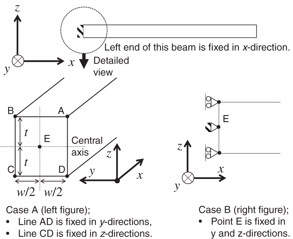
Figure 5: Boundary conditions at left end of bimorph

4.1 Problem Setup

The piezoelectric actuator model presented in Section 2.3 is used here. The piezoelectric bimorph in Fig. 1 has a length of L = 20 mm, a layer thickness of t = 0.25 mm, and a width of w = 1, 2, …, and 7 mm. The finite element meshes use 20-node hexahedral elements and are equally divided into 40 regions along the length direction (x-axis) and 4 regions along the thickness direction (z-axis). The numbers of mesh divisions along the width direction (y-axis) are 2, 4, 8, 10, 12, and 14 for w = 1, 2, 4, 5, 6, and 7 mm, respectively, and thus all elements have the same aspect ratio. The material properties of the PZT with the highest k31 in Table 1 (P-15) are used in this section. The external voltage applied to the bimorph is 1 V. A roller support is imposed on the fixed end of the bimorph (Case A in Fig. 5).

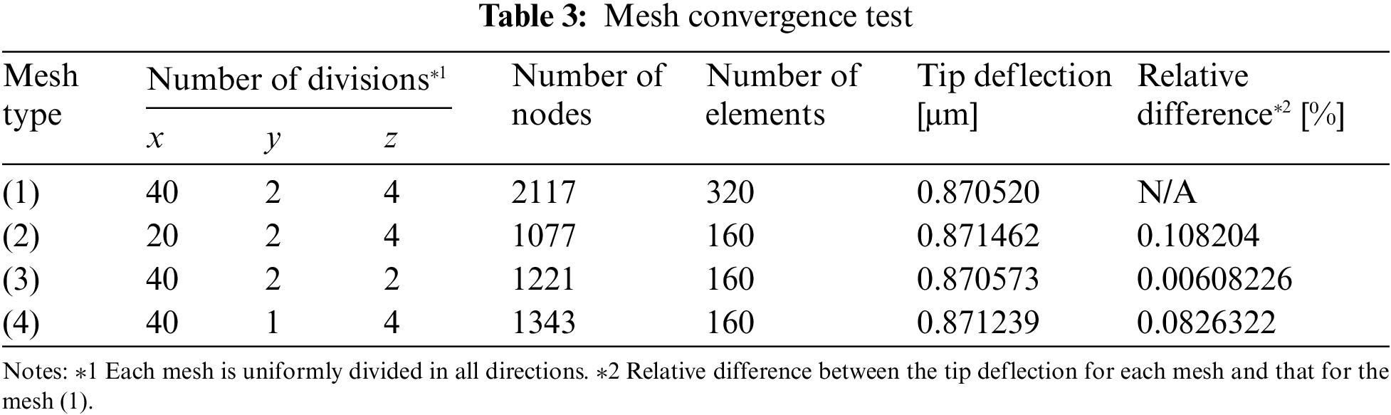
In order to check the mesh convergence, the bimorph with the P-15 material in Table 1 and w = 1 mm is analyzed using the numerical weak coupling solution. The results are summarized in Table 3, where the mesh type (1) corresponds to the above meshes. As shown in this table, the relative difference among the tip deflections is sufficiently small. Hence, in the following section, the above meshes are used.

4.2 Results and Discussion

4.2.1 Three-Dimensional Inverse-Piezoelectric Effect

The weak coupling analysis using the 3-D finite element method described in Section 2.2 and the theoretical solution based on the Euler-Bernoulli beam assumption (Eq. (33)) are applied for the problem in Section 4.1. Their formulations are based on the weak coupling model that ignores the DPE (i.e., it uses only the IPE). In the pure elastic bending analysis for the present problem setup, the theoretical solution based on the Euler-Bernoulli beam assumption agrees well with the 3-D finite element analysis result. Hence, the difference between the numerical weak coupling solution and the theoretical solution is caused only by the 3-D IPE. This effect can be described in terms of the piezoelectric constitutive equations using the strain-electric displacement form S = dTE as

{S1S2S3S4S5S6}=[00d3100d3100d330d150d1500000]{00E3}={d31E3d31E3d33E3000}(35)

where S, d, and E are given as

ST=[S1S2S3S4S5S6](36)

d=[d11d12d13d14d15d16d21d22d23d24d25d26d31d32d33d34d35d36]=[0000d150000d15d250d31d31d33000](37)

and

ET=[E1E2E3]=[00E3](38)

Fig. 6 plots the relative difference between the tip displacement in the z-direction given by the numerical weak coupling solution and that given by the theoretical solution (Eq. (33)) for the beam width. Note that the numerical result is taken at the center point of the section at the tip because the numerical result shows bending deformation along the y-direction. Fig. 7 shows the bending deformation along the y-direction, where the tip displacement in the z-direction is plotted along the central axis for each width of the beam. The difference shown in Fig. 6 increases almost linearly with increasing beam width. Note that this difference is sufficiently small when the width is close to the thickness. Importantly, this figure shows the necessity of the 3-D IPE analysis. The following section elucidates how this effect causes the difference shown in the figure.

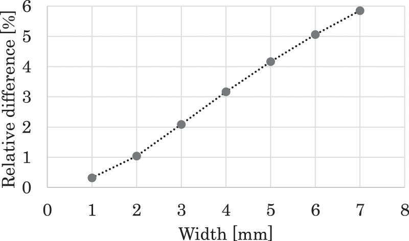
Figure 6: Relationship between width and relative difference between z displacements at tip given by theoretical and numerical solutions

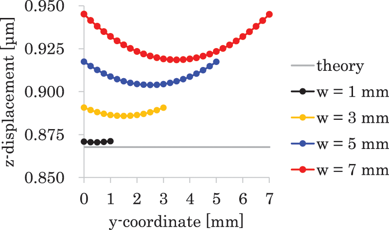
Figure 7: Deformation along width direction or z-displacement at tip plotted along central axis. In the numerical weak coupling analysis, the 3-D inverse piezoelectric effect was considered

4.2.2 Inverse Piezoelectric Effect in Length and Width Directions

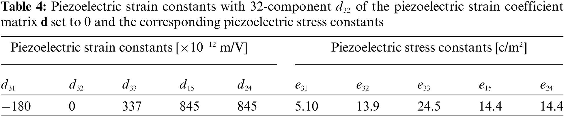
First, we set the 32-component d32 of the piezoelectric strain coefficient matrix d in the 3-D IPE (see Eq. (37)) to 0. Then, we remove the IPE in the width direction based on Eq. (35) as

{S1S2S3S4S5S6}=[00d3100000d330d150d1500000]{00E3}={d31E30d33E3000}(39)

The piezoelectric strain constant d and the corresponding piezoelectric stress constant e, obtained using Eq. (27), are shown in Table 4. In this case, the tip displacement in the z-direction is 0.8637 μm for w = 1, 3, 5, and 7 mm; the theoretical solution is 0.8640 μm (approximately 0.04% higher). Note that the theoretical solution uses only the IPE in the length direction.

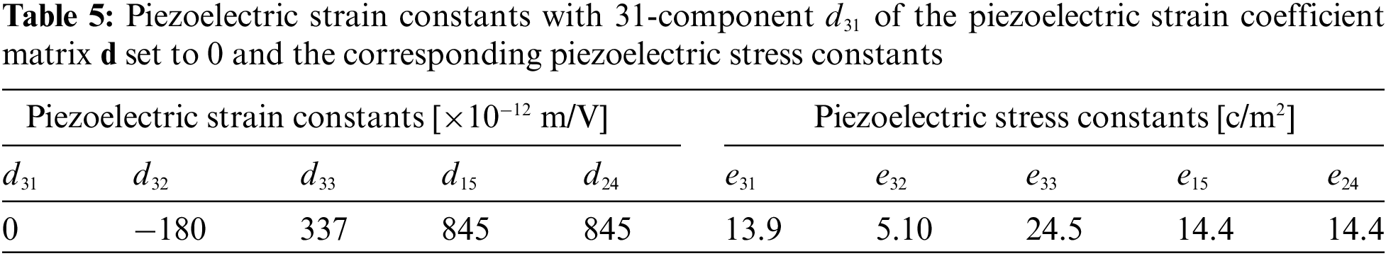
Next, we set the 31-component d31 of the piezoelectric strain coefficient matrix d in the 3-D IPE (see Eq. (37)) to 0. Then, we remove the IPE in the length direction based on Eq. (35) as

{S1S2S3S4S5S6}=[00000d3100d330d150d1500000]{00E3}={0d31E3d33E3000}(40)

The piezoelectric strain constant d and the corresponding piezoelectric stress constant e, obtained using Eq. (27), are shown in Table 5. There is bending deformation along the width direction, as shown in Fig. 8A, which shows the tip displacement in the z-direction plotted along the central axis for each beam width. This deformation causes bending deformation along the length direction, as shown in Fig. 8B, which shows the displacement in the z-direction plotted along the longitudinal axis between the center of the section at the fixed end and that at the free end.

The superposition of the numerical solution with the IPE in the length direction and the numerical solution with the IPE in the width direction is very close to the numerical solution with the 3-D IPE (the difference is approximately 0.04%). These results indicate that the difference between the weak coupling solution with the 3-D IPE and the theoretical solution is caused by the IPE in the width direction.

4.2.3 Longitudinal Bending Mechanism Due to Inverse-Piezoelectric Effect in Width Direction

In the previous section, we demonstrated that the IPE in the width direction causes longitudinal bending deformation. In this section, this mechanism is discussed. For a width of w = 7 mm, the overall deformations due to the IPE in the width direction using the boundary conditions for Cases A and B in Fig. 5 are considered. It should be noted here that Case A used in the previous sections does not allow bending deformation along the width direction at the fixed end, whereas Case B allows it. Figs. 10A and 10B show the overall deformations for Cases A and B, respectively. The deformation in Case A can be understood as a transition from Case B using an idea similar to that for thermal stress and strain.

In the first step, the deformation from the initial position in Case B occurs due to the IPE in the width direction. In this case, as shown in Fig. 9B, there is bending deformation along the width direction, and this deformation is almost uniform along the longitudinal direction. In the second step, forced displacement in the thickness direction is applied to the fixed end such that it satisfies the boundary condition for Case A. During this transition, with respect to the xz-plane of the symmetry shown in Fig. 9B, the two halves of this structure support each other via the action-reaction law. Hence, the forced displacement that pushes down the fixed end generates a clockwise moment about the width direction, which causes bending deformation along the length direction, as shown in Fig. 9A. Hence, the plate is twisted from both sides to form the concave near the midpoint of the fixed end as shown in Fig. 9A, which corresponds to the negative z-displacement in Fig. 8B.

Figure 8: The z-displacement at tip plotted along central axis (A), and the z-displacement plotted along longitudinal axis between center of section at the fixed end and that at free end (B). In this weak coupling analysis, the inverse piezoelectric effect in the length direction S1 = d31E3 was removed and that in the width direction S2 = d31E3 was kept

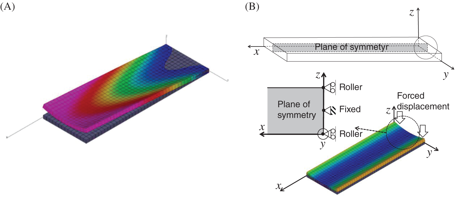
Figure 9: Overall deformations in Cases A and B (see Fig. 5). The color contours show the magnitude of the z-displacement

To confirm this interpretation, we consider a problem similar to the second step of this process, as shown in Fig. 10A. In this figure, a roller support is imposed at the left end of the xz-plane of the symmetry, and the force displacement is applied at the corner points along the thickness direction. Here, with respect to the xz-plane of the symmetry shown in Fig. 10A, the two halves of this structure support each other via the action-reaction law. Hence, the forced displacement that pushes down the corners generates a clockwise moment about the y-axis. This causes a tip displacement in the z-direction, as shown in Fig. 10B.

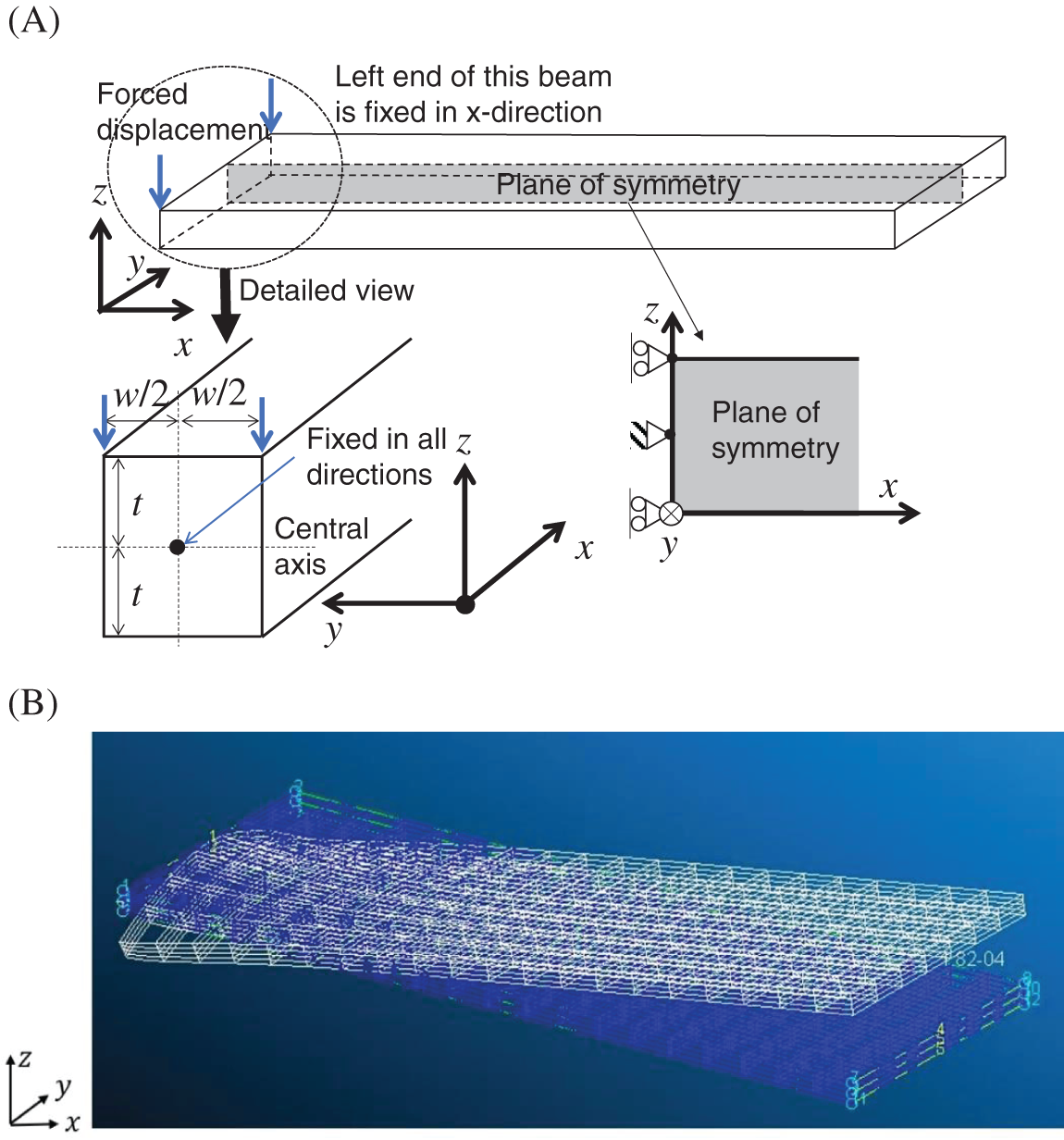
Figure 10: Bending deformation along length direction (A) caused by forced displacement along thickness direction (B)

4.2.4 Three-Dimensional Piezoelectric Coupling Analysis

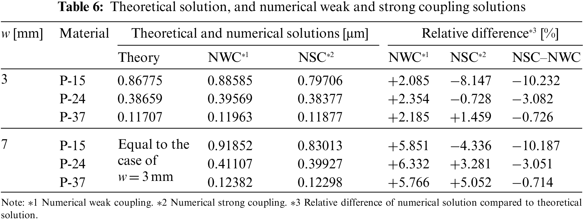
Tip bending displacements are given by theoretical, numerical weak coupling (NWC) and numerical strong coupling (NSC) solutions for the materials P-15, P-24, and P-37 (see Table 1) are summarized in Table 6, where the widths of w = 3 and 7 mm are used. We discuss the piezoelectric coupling effect (PCE) and the 3-D IPE using this table. As shown in the previous sections, the PCE decreases bending magnitude compared to the theory, and the 3-D IPE increases it compared to the theory. Assuming that the NSC solution is the superimposition of the two effects, we can evaluate the PCE by substituting the NWC solution from the NSC solution because the NWC solution is only the 3-D IPE. As shown in Table 6, the PCEs are evaluated as approximately −10.2% for P-15, −3.1% for P-24, and −0.7% for P-37 for both the widths of w = 3 and 7 mm. The IPEs are approximately + 2% for w = 3 mm and + 6% for 7 mm. We can understand the electromechanical behaviors of the cantilevered piezoelectric bimorph actuator in more detail using the 3-D piezoelectric coupling analysis above. In the case of w = 3 mm and P-24 in Table 6, the NSC solution is very close to the theoretical solution, and this is because the magnitudes of the PCE and the 3-D IPE are almost equivalent to each other and their sign is opposite (i.e., the former is approximately −3.1% and the latter is + 2.4%).

4.2.5 Comparison with the Experiment

Fig. 11 shows the relationship between the in-plane aspect ratio RA and the tip displacement along the z-direction given by the results in Section 4.2.1, where RA is defined as the ratio of the length to the width of the bimorph. In this figure, the numerical and theoretical solutions are distinguishable from each other for RA smaller than 5. Furthermore, in this range of RA, the numerical solution is larger than the theoretical solution, and their difference increases as RA decreases. In an experimental and theoretical study of the quasistatic response of the piezoelectric bimorph [12], the experimental results clearly show the same behavior for the theoretical solution. However, in previous studies, the mechanism of this characteristic behavior has not been discussed in detail as long as we know. On the contrary, this study revealed this characteristic behavior can be caused by the constraint of the bending along the width direction due to the IPE.

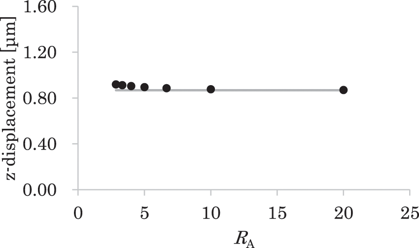
Figure 11: Relationship between the square of the aspect ratio RA and the z-displacement at the tip of the bimorph, where the RA is the ratio of the length and the width. The black circle corresponds to the numerical result, and the grey line corresponds to the theoretical solution

Fig. 12 shows the relationship between RA and the bowing at the tip of the bimorph, where the bending is the bending deformation along the width direction, the magnitude of the bowing is defined as the relative difference of the corner and midpoint displacements along the z-direction at the tip of the bimorph. The magnitudes of the bowing for RA = 5 in the present numerical result and the previous experimental result [12] are 0.97% and 1%, respectively, which are very close to each other. As shown in Fig. 12, the bowing exceeds about 1% for RA smaller than 5, and it becomes significant as RA decreases. This change of the bowing for RA correlates highly with the above-mentioned characteristic behaviors in the present computation and the previous experiment [12].

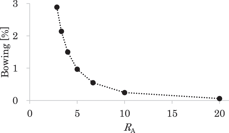
Figure 12: Relationship between the aspect ratio RA and the bowing at the tip, where the RA is the ratio of the length and the width, the bowing is the bending along the width direction, and the magnitude of the bowing is evaluated as the relative difference of the corner and midpoint displacements along the z-direction at the tip of the bimorph

5  Concluding Remarks

This study demonstrated the importance of 3-D piezoelectric coupling modeling for accurate predictions of the electromechanical behavior of piezoelectric devices. 3-D finite element analysis methods based on weak and strong coupling models were compared using a thin cantilevered piezoelectric bimorph actuator. An important difference between the strong coupling model for the numerical analysis and the weak coupling model for the numerical and theoretical analyses was that the former solution included the coupling of the DPE and the IPE (i.e., the piezoelectric coupling) accurately, whereas the latter solutions included only the IPE. Furthermore, an important difference between the numerical weak coupling solution and the theoretical solution was that the former included the 3-D IPE, whereas the latter included only the longitudinal IPE.

The present results can be summarized as follows. For a thin cantilevered piezoelectric bimorph actuator, the difference between the strong and weak coupling solutions given by piezoelectric coupling is almost proportional to the electromechanical coupling coefficient. This difference is significant for actual materials. In addition, the longitudinal bending caused by the constraint of the IPE in the width direction at the fixed end is almost proportional to the width dimension, and its contribution to the total longitudinal bending cannot be ignored even for a geometrical configuration where the Euler-Bernoulli beam assumption holds for the mechanical constitutive relationship. The results show that 3-D piezoelectric coupling modeling is important for the accurate analysis of typical piezoelectric devices such as a thin cantilevered piezoelectric bimorph actuator. In addition, the strength of the piezoelectric coupling can be quantitatively measured using the electromechanical coupling coefficient.

Funding Statement: This research was supported by the Japan Society for the Promotion of Science under KAKENHI Grant Nos. 19F19379 and 20H04199.

Conflicts of Interest: The authors declare that they have no conflicts of interest to report regarding the present study.

References

1. Tuloup, C., Harizi, W., Aboura, Z., Meyer, Y., Khellil, K. et al. (2019). On the use of in-situ piezoelectric sensors for the manufacturing and structural health monitoring of polymer-matrix composites: A literature review. Composite Structures, 215, 127–149. DOI 10.1016/j.compstruct.2019.02.046. [Google Scholar] [CrossRef]
2. Shirbania, M. M., Sedighia, H. M., Ouakadb, H. M., Najar, F. (2018). Experimental and mathematical analysis of a piezoelectrically actuated multilayered imperfect microbeam subjected to applied electric potential. Composite Structures, 184, 950–960. DOI 10.1016/j.compstruct.2017.10.062. [Google Scholar] [CrossRef]
3. Chee, C., Tong, L., Steven, G. P. (1988). A review on the modelling of piezoelectric sensors and actuators incorporated in intelligent structures. Journal of Intelligent Material Systems and Structures, 9(1), 3–19. DOI 10.1177/1045389X9800900101. [Google Scholar] [CrossRef]
4. Nguyen, C. H., Pietrzko, S. J. (2006). FE analysis of a PZT-actuated adaptive beam with vibration damping using a parallel R-L shunt circuit. Finite Elements in Analysis and Design, 42(14–15), 1231–1239. DOI 10.1016/j.finel.2006.06.003. [Google Scholar] [CrossRef]
5. Sun, H., Yang, Z., Li, K., Li, B., Xie, J. et al. (2009). Vibration suppression of a hard disk driver actuator arm using piezoelectric shunt damping with a topology optimized PZT transducer. Smart Materials and Structures, 18(6), 065010. DOI 10.1088/0964-1726/18/6/065010. [Google Scholar] [CrossRef]
6. Matsuda, H., Tanaka, Y., Patel, R., Doi, Y. (2017). Harvesting flow-induced vibration using a highly flexible piezoelectric energy device. Applied Ocean Research, 68, 39–52. DOI 10.1016/j.apor.2017.08.004. [Google Scholar] [CrossRef]
7. Pan, D., Ma, B., Dai, F. (2017). Experimental investigation of broadband energy harvesting of a bi-stable composite piezoelectric plate. Smart Materials and Structures, 26(3), 035045. DOI 10.1088/1361-665X/aa5b41. [Google Scholar] [CrossRef]
8. Erturk, A., Inman, D. J. (2011). Piezoelectric energy harvesting. England: John Wiley & Sons, Ltd. [Google Scholar]
9. Karpelson, M., Wei, G. Y., Wood, R. J. (2008). A review of actuation and power electronics options for flapping-wing robotic insects. 2008 IEEE International Conference on Robotics and Automation, pp. 779–786. Pasadena, California. [Google Scholar]
10. Ishihara, D., Ohira, N., Takagi, M., Horie, T. (2017). Fluid-structure interaction design of insect-like micro flapping wing. Proceeding of the VII International Conference on Computational Methods for Coupled Problems in Science and Engineering, pp. 870–875. Rhodes Island, Greece. [Google Scholar]
11. Ishihara, D. (2022). Computational approach for the fluid-structure interaction design of insect-inspired micro flapping wings. Fluids, 7(26), 7010026. DOI 10.3390/fluids7010026. [Google Scholar] [CrossRef]
12. Steel, M. R., Harrison, F., Harper, P. G. (1978). The piezoelectric bimorph: An experimental and theoretical study of its quasistatic response. Journal of Physics D: Applied Physics, 11(6), 979–989. DOI 10.1088/0022-3727/11/6/017. [Google Scholar] [CrossRef]
13. Wang, Q. M., Du, X., Xu, B., Cross, L. E. (1999). Theoretical analysis of the sensor effect of cantilever piezoelectric benders. Journal of Applied Physics, 85(3), 1702–1712. DOI 10.1063/1.369314. [Google Scholar] [CrossRef]
14. Erturk, A., Inman, D. J. (2009). An experimentally validated bimorph cantilever model for piezoelectric energy harvesting from base excitations. Smart Materials and Structures, 18(2), 025009. DOI 10.1088/0964-1726/18/2/025009. [Google Scholar] [CrossRef]
15. Benjeddou, A. (2000). Advances in piezoelectric finite element modeling of adaptive structural elements: A survey. Computers & Structures, 76(1), 347–363. DOI 10.1016/S0045-7949(99)00151-0. [Google Scholar] [CrossRef]
16. Fish, J., Chen, W. (2003). Modeling and simulation of piezo composites. Computer Methods in Applied Mechanics and Engineering, 192(28), 3211–3232. [Google Scholar]
17. Amini, Y., Emdad, H., Farid, M. (2015). Finite element modeling of functionally graded piezoelectric harvesters. Composite Structures, 129, 165–176. DOI 10.1016/j.compstruct.2015.04.011. [Google Scholar] [CrossRef]
18. Wu, P. H., Shu, Y. C. (2015). Finite element modeling of electrically rectified piezoelectric energy harvesters. Smart Materials and Structures, 24(9), 094008. DOI 10.1088/0964-1726/24/9/094008. [Google Scholar] [CrossRef]
19. Elvin, N. G., Elvin, A. A. (2009). A coupled finite element-circuit simulation model for analyzing piezoelectric energy generators. Journal of Intelligent Material Systems and Structures, 20(5), 587–595. DOI 10.1177/1045389X08101565. [Google Scholar] [CrossRef]
20. Junior, C. D. M., Erturk, A., Inman, D. J. (2009). An electromechanical finite element model for piezoelectric energy harvester plates. Journal of Sound and Vibration, 327(1–2), 9–25. DOI 10.1016/j.jsv.2009.05.015. [Google Scholar] [CrossRef]
21. Ramegowda, P. C., Ishihara, D., Niho, T., Horie, T. (2019). Performance evaluation of numerical finite element coupled algorithms for structure–electric interaction analysis of MEMS piezoelectric actuator. International Journal of Computational Methods, 16(7), 1850106. DOI 10.1142/S0219876218501062. [Google Scholar] [CrossRef]
22. Ramegowda, P. C., Ishihara, D., Niho, T., Horie, T. (2019). A novel coupling algorithm for the electric field-structure interaction using a transformation method between solid and shell elements in a thin piezoelectric bimorph plate analysis. Finite Elements in Analysis and Design, 159, 33–49. DOI 10.1016/j.finel.2019.02.001. [Google Scholar] [CrossRef]
23. Ramegowda, P. C., Ishihara, D., Takata, R., Niho, T., Horie, T. (2020). Hierarchically decomposed finite element method for a triply coupled piezoelectric, structure, and fluid fields of a thin piezoelectric bimorph in fluid. Computer Methods in Applied Mechanics and Engineering, 365, 113006. DOI 10.1016/j.cma.2020.113006. [Google Scholar] [CrossRef]
24. Ishihara, D., Takata, R., Ramegowda, P. C., Takayama, N. (2021). Strongly coupled partitioned iterative method for the structure–piezoelectric–circuit interaction using hierarchical decomposition. Computers & Structures, 253, 106572. DOI 10.1016/j.compstruc.2021.106572. [Google Scholar] [CrossRef]
25. Ramegowda, P. C., Ishihara, D., Takata, R., Niho, T., Horie, T. (2020). Finite element analysis of a thin piezoelectric bimorph with a metal shim using solid direct-piezoelectric and shell inverse-piezoelectric coupling with pseudo direct-piezoelectric evaluation. Composite Structures, 245, 112284. DOI 10.1016/j.compstruct.2020.112284. [Google Scholar] [CrossRef]
26. Tan, X. G., Vu-Quoc, L. (2005). Optimal solid shell element for large deformable composite structures with piezoelectric layers and active vibration control. International Journal for Numerical Methods in Engineering, 64(15), 1981–2013. DOI 10.1002/(ISSN)1097-0207. [Google Scholar] [CrossRef]
27. Lenger, D., Klinkel, S., Wagner, W. (2013). An advanced finite element formulation for piezoelectric shell structures. International Journal for Numerical Methods in Engineering, 95(11), 901–927. DOI 10.1002/nme.4521. [Google Scholar] [CrossRef]
28. Ishihara, D., Horie, T. (2014). A projection method for the monolithic interaction system of an incompressible fluid and a structure using a new algebraic splitting. Computer Modeling in Engineering & Sciences, 101(6), 421–440. DOI 10.3970/cmes.2014.101.421. [Google Scholar] [CrossRef]
29. Moulson, A. J., Herbert, J. M. (2003). Electroceramics (second edition). England: John Wiley & Sons, Ltd. [Google Scholar]
30. Xu, T. B. (2016). Energy harvesting using piezoelectric materials in aerospace structures. Structural Health Monitoring in Aerospace Structures, 175–212. DOI 10.1016/B978-0-08-100148-6.00007-X. [Google Scholar] [CrossRef]
31. Uchino, K. (2012). Piezoelectric ceramics for transducers. Ultrasonic Transducers, 70–116. DOI 10.1533/9780857096302.1.70. [Google Scholar] [CrossRef]
Cite This Article
Copyright © 2023 The Author(s). Published by Tech Science Press.
This work is licensed under a Creative Commons Attribution 4.0 International License , which permits unrestricted use, distribution, and reproduction in any medium, provided the original work is properly cited.
Downloads
Citation Tools