The Influence of Saturated and Bilinear Incidence Functions on the Dynamical Behavior of HIV Model Using Galerkin Scheme Having a Polynomial of Order Two

1  Introduction

The study of epidemic models is a powerful tool for the dynamics of different infectious diseases in real-world phenomena. For the transmission dynamics of infectious diseases in a population, mathematicians and biologists used various epidemic models [1–4]. There are innovative scientific advances and significant health intervention measures in the globe, yet HIV/AIDS remains one of humanity’s graves devastating diseases. Many countries are still seriously afflicted by this disease. Currently, the global spread of HIV infection is influencing the occurrence of other infectious diseases such as tuberculosis (TB) [2]. HIV is a virus that causes HIV infection and is transferred during sexual activity, breastfeeding, and sharing injectable drug gear such as needles with HIV positive people. AIDS, the most severe stage of HIV infection, is triggered by the HIV pathogens. In 2018, the number of individuals living with HIV/AIDS and the number of deaths worldwide is expected to hit 37.9 million and 1.2 million, respectively. Approximately 62% of those infected were confirmed and started on antiretroviral therapy (ART) [4]. Many therapies have been proposed to improve the quality of life of HIV patients, including antiretroviral therapy [5], chemotherapy, and stem cell therapy. Antiretroviral therapy, which is the most commonly used combination of drugs to treat HIV infection, has many side effects [6]. Stem cell therapy is very limited due to the high cost of the procedure as well as the difficulty of obtaining healthy and consistent donors. A mathematical model is a mathematically based description of a dynamical system. It is essential for evaluating and controlling the HIV/AIDS infectious disease. Several assumptions and factors have substantial effects on the construction of a model, which may be changed employing controlling functions. Thus, using the idea of optimal control theory, a mathematical model of the HIV/AIDS pandemic can be reconstructed, and the disease’s regulating mechanisms may be studied. This theory contains several useful concepts that explain how disease, whether epidemic or pandemic, may be managed via biological controls. This concept has been adopted by many authors in order to control infection. Several HIV models have been developed in recent years to better understand the dynamics of HIV infection, disease progression, and the interaction of the immune system with HIV in the area of HIV infection of CD4+T cells.

Naresh et al. [7] presented a nonlinear HIV/AIDS mathematical model. They claimed that HIV infection has been reduced significantly because of increased awareness of HIV infectives as identified by screening and contact tracing, but that the illness remains prevalent due to immigration and the lack of contact tracking. Finally, they believe that the most effective way to minimize the disease burden is to spread awareness about HIV/AIDS. Nyabadza et al. [8] investigated a deterministic HIV/AIDS model that describes condom usage, HIV counselling and testing (HCT), and therapy. They examined the concept because HCT practice is still in its early stages. According to the model, this campaign has very little impact on reducing HIV endemicity. A mathematical model for HIV/AIDS dynamics was proposed by Mushanyu [9]. He looked at the effects of HIV late diagnosis on the disease’s spread. His numerical findings show that early HIV/AIDS treatment motivation and improved HIV self-testing schedules offer more undiagnosed people the knowledge they need to know their HIV status, reducing HIV transmission. Ullah et al. [10] established an optimal control model for the COVID-19 pandemic. They used real-world data to quantitatively evaluate the model. They proved that the proposed method could control the disease. Geffen et al. [11] proposed a mathematical model of the hepatitis B virus, including isolation, treatment, and vaccine technology. Alrabaiah et al. [12] used the Galerkin method to solve the HIV infection model. They used a method called residual correction. The purpose of this technique is to reduce the error rate of the solution. Yüzbaşı et al. [13] used the cGP (2) and “LWCM” to approximate the solution of the proposed model. Furthermore, they solved the model using the traditional RK4-method. Finally, they compared the results obtained from the RK4-method to those acquired from the proposed schemes in order to ensure their validity. Sohaib [14] came up with a completely new way to think about the HIV pandemic. This model allows for a lot of new people to get infected. They examined the impact of public health education initiatives on the prevalence of the condition and found that they had no effect. In order to define the control and determine the best system, they employed “Pontryagin’s maximal principle”. Seatlhodi [15] developed and tested HIV/AIDS models using Caputo-fractional derivatives as a medical therapy. They first established Caputo-fractional order HIV/AIDS models with switching parameters and studied their dynamics using the Lyapunov–Razumikhin approach, based on the fractional derivative order linked to memory and genetic effects, and considering that the model coefficients are time-varying parameters. Wang et al. [16] proposed an SIR model with long-range temporal memory. The proposed model consists of delayed differential equations. They considered that the susceptible individual is following the logistic form, in which the incidence term takes the saturated form. The existence of steady states and the stability of those states are also examined. The concept of the Lyapunov function is used to figure out a new set of conditions that keep the steady states stable. The dynamical behavior of various infectious diseases are described using the idea of mathematical modeling (see [17–30] for detail information). Attaullah et al. [31] established a mathematical model for the dynamics of Human Immunodeficiency Virus (HIV) infection. They implemented the continuous Galerkin Petrov time discretization scheme and a fourth-order Runge-Kutta (RK4)-method to illustrate the dynamical behavior of the model, as well as a detailed description of the effects of different physical parameters of interest, which are depicted graphically and discussed how the level of healthy, infected CD T-cells, and free HIV particles varies related to the emerging parameters in the model. Sabir et al. [32] considered a novel designed prevention class in the HIV nonlinear model and solved numerically. Amin et al. [33] used the Haar wavelet approach to estimate the solution of the mathematical model of HIV infection CD4+T-Cells.

In this manuscript, we implemented a new method, namely the continuous Galerkin-Petrov scheme for finding the approximate solution of the non-linear model for HIV infection presented by Mehdi et al. [1]. The proposed model is divided into four different compartments. We presented the impact of saturated and bilinear incidence functions and different clinical parameters (the parameter φ shows the default treatment rate for the individual, ζ is concerned with HIV treatment rate for the individual) on the dynamical behavior of the model. The present findings are conducive in the field of mathematical modeling of HIV infection of CD4+T-cells. This will be used to analyzed the population dynamics of CD4+T-cells in the presence and absence of HIV, helpful to observe the symptoms of AIDS seen clinically and valuable to hold back the disease. Medically, it provides sufficient information to clinicians to reduce the viral load of the infection.

2  Mathematical Description of the Model

In the absence of HIV, it is important to understand the population of T-cells produced by the bone marrow. Therefore, the premature cells shifted to an organ called the thymus, which is present in the chest sternum for further maturation and conversion into immune component T-cells. In humans, at the time of puberty, the thymus secretion in adults has minimal consequences, despite the thymus being in full operation and the fever lymphocytes performing as precursors of T-cells and immune component T-cells. The progression chain can be calculated by the number of T-cells, which shows us the initial symptoms. Enormous models have been developed for HIV infection. Mehdi et al. [1] suggested that the HIV infection model consists of four variables as follows:

dSdt=λ−γS(t)−ψ(S(t),I(t))I(t),(1)

dIdt=ψ(S(t),I(t))I(t)−(φ+ζ+γ)I(t)+εA(t)+σC(t),(2)

dCdt=ζI(t)−(σ+γ)C(t),(3)

dAdt=φI(t)−(ε+γ+η)A(t)(4)

initial conditions are given as follows:

S(0)=S0≥0,I(0)=I0≥0,C(0)=C0≥0,A(0)=A0≥0,(5)

the unknows S(t),I(t),C(t),A(t) illustrate the susceptible individuals, HIV infected individuals (with no clinical symptoms of AIDS), HIV infected individuals (under ART treatment with a viral load remaining low) and HIV infected individuals, respectively. The detailed description of the parameters used in the model are presented in Table 1.

The general incidence function ψ(S,I) which is assumed to depend on the effective contact rate ρ>0. Then,ψ can take many forms. Table 2 is composed of some special incidence functions.

3  The Continuous Galerkin Petrov Technique

The Galerkin technique is an effective tool for numerically investigating critical challenges. This approach is commonly employed for complicated problems and is capable of dealing with nonlinear system and complicated problems.

This section is focused on the application and implementation of the suggested technique to the aforementioned model. For simplicity some assumptions are given, i.e., u1(t)=S(t),u2(t)=I(t),u3(t)=C(t),u4(t)=A(t), initially at t=0,

u1(0)=S(0)=ρ1,u2(0)=I(0)=ρ2,u3(0)=C(0)=ρ3,u4(0)=A(0)=ρ4.

Find u:J=[0,T]→V. Here J = [0,T] describes the time interval, for function

u:J×V→ and t∈T

dtu(t)=ψ(t,u(t))∀t∈J=[0,T]u(0)=u0,(6)

Here dtu(t) refers to the time derivative of u(t). The derivative of u(t) w.r.t tu(t)= (u1(0),u2(0),u3(0))∈V represents u(t) at t = 0, and ψ=(ψ1,ψ2,ψ3) and describes as ψ:J×V→V. The formulation of Eq. (6) is: find u∈X′ such that u(0)=uo and

∫J⟨dtu(t),ϑ(t)⟩dt=∫J⟨ψ(t,u(t),ϑ(t)⟩dtforallϑ∈Y′,(7)

where X′, and Y′ represent the solution space and the test space respectively. To describe function t→u(t), we consider the space E(J ,V)=EO(J,V) as the space of contionuous functions u:J→V equipped with norm

||u||E(J ,V)=EO(J ,V)=supt∈=[0,T]||u(t)||V.

M2(J,V) represents the space of square integrable function M2(J ,V) by containing discontinuous functions, which is expressed in the form as M2(J ,V)={u:[0,T]→V:||u||M2(J ,V)<∞} with ||u||M2(J ,V)=(∫J||u(t)||V2dt)12

We divide the time interval J into N subintervals for the Galerkin time discretization. Jn=[tn−1,tn], where n=1,2,3,…,N, and 0 = t0<t1<…tN−1<tn=T. The symbol τ denotes the time discretization parameter, which will be used to determine the maximum time step size τ=max1≤n≤Nτn, where τn=tn−tn−1, which is the length of each Jn. Now we will approximate u:J→V using a function uτ:J→V (see [14,26,27,30,31] for details). Then, we will find the space for

Xτ′l={u∈E(J→V):u|Jn∈Hl(Jn,V)for all Jn∈Gτ},

where Hl(Jn,V)={u:Jn→V,u(t)=∑j=0lUjtj,∀t∈Jn,Uj∈V,forallj}, and the test space for uτ is Yτk, illustrated as:

Y′τl={V∈M2(J,V):V|Jn∈Hl−1(Jn,V)for all Jn∈Gτ},

where Y′τl consists of piecewise polynomials of order l−1, which are discontinuous at the end points of the time intervals. By taking a test function ϑτ∈Y′τl and multiplying it by Eq. (6) , and integrate over J (see [14,26,27,30] for details). Find uτ∈X′τl such that uτ(0)=0 and

∫J⟨dtuτ(t),ϑτ(t)⟩dt=∫J⟨ψ(t,uτ(t)),ϑτ(t)⟩dt∀ϑτ∈Y′τl.(8)

This discretization is called the exact cGP-technique of order l. (see [14,22–31] for details). Now, to find u|Jn∈Hl(Jn,V) such that

∫Jn⟨dtuτ(t),ϑ⟩φ(t)dt=∫Jn⟨φ(t,uτ(t)),ϑ⟩φ(t)dt∀ϑ∈Vand∀φ∈H(Jn),(9)

with the initial condition uτ|Jn(tn−1)=uτ|Jn−1(tn−1), for n≥2 and uτ|Jn(tn−1)=u0 for n=1. As a general case of a nonlinear function ψ⟨.,.⟩, we approximate the integral on the right-hand side of Eq. (9) by the (l+1)-points Gauss-Lobatto quadrature formula (see [14,22–31] for details). Find

u|Jn∈Hl(Jn,V), such that

uτ(tn−1)=un−1

∑j=0lwjdtuτ(tn,j)φ(tn,j)=∑j=0lwjψ(tn,j,uτ(tn,j))φ(tn,j)∀φ∈Hk−1(Jn),(10)

where wj are the weights.

To determine uτ|Jn, we represent it by a polynomial ansatz

uτ(t)=∑j=0lUnj∅n,j(t)∀t∈Jn(11)

where the coefficient Unj is the elements of V and the real valued function ∅n,jH(Jn) are the Lagrange basis functions with respect to (l+1) suitable nodal points tn,j∈Jn satisfying the conditions.

∅n,j(tn,j)=δi,j,i,j=0,1,2,…,l,(12)

where δi,j is the Kronecker delta that is

δi,j={1:ifi=j0:ifi≠j.

For the choice of initial conditions, we set tn,0 = tn−1, which implies that the initial conditions for Eq. (9) is given as

Un0=uτ|Jn(tn−1),ifn≥2,

Un0=u0,ifn=1.(13)

The other points tn,1,tn,2,…,ttn,l are chosen as the quadrature points of the l-points Gauss-Lobatto formula on the time interval Jn. For representation (11), for dtuτ, we get

dtuτ=∑j=0lUnj∅′n,j(t),∀t∈Jn,(14)

Using Eq. (14) in Eq. (9), we get

∫Jn⟨dtuτ(t),ϑ⟩φ(t)dt=∫Jn⟨∑j=0lUnj,ϑ⟩∅′j(t)φ(t)dt.

This implies that

∫Jn⟨dtuτ(t),ϑ⟩φ(t)dt=∑j=0l⟨Unj,ϑ⟩∫Jn∅′j(t)φ(t)dt.(15)

We define the basis functions ∅n,j∈Hk(Jn) via the affine reference transformation

ϖn: J^→Jn, where J^=[−1,1] and

t=ϖnt^=tn+tn−12+τn2t^∈Jn∀t^∈J^,n=1,2,3,…,N.(16)

Let ∅^j∈Hk(J^), j=0,1,2,…,l, denote the basis functions satisfying the conditions

∅^(t^i)=δi,j,i,j=0,1,2,…,l,(17)

where t^0=−1andt^i,i=1,2,3,…,l, are the quadrature points for the interval J^. Then, we define the basis functions on the original time interval Jn by the mapping

∅n,j(t)=∅^j(t^)witht^=ϖn−1(t)=2τn(t+tn−1−tn2)∈J^.

Similarly, we define the test basis functions φn,i by suitable reference basis functions

φ^i∈Hl−1(J^), i.e.,

φn,i(t)=φ^i(ϖn−1(t)∀t∈Jn,i=1,2,3,…,l.(18)

Now, we transform the integral into a reference interval J^=[−1,1] and approximate it by the (l+1) point Gauss-Lobatto quadrature formula which leads, for each test basis function φ∈Hl−1 and for all ϑ∈V, to the following:

∫J^n∑j=0l⟨Unj,ϑ⟩∅^j′(t^)φ^(t^)dt^=τn2∫J^n⟨ψ(ωn(t^),∑j=0lUnj(t^)),ϑ⟩φ^(t^)dt^∀ϑ∈V.

This implies that

∑μ=0lϖμ^∑j=0l⟨Unj,ϑ⟩∅^j′(t^μ)φ^(t^μ)=τn2∑μ=0lϖμ^⟨ψ(ωnt^μ,∑j=0lUnj(t^μ)),ϑ⟩φ^(t^μ).(19)

Here ϖμ^ are the weights and t^μ∈ [1, −1] are the integration points with the t^0=−1 and t^l=1

φ^i(t^μ)=(ϖμ^)−1δi,μi,μ={1,2,3,…,l}.(20)

Then we get the special form of the numerically integrated J^n-problem of cGP (k), find the l unknown coefficients Unj∈V where j=1,2,3,…,l, such that

∑j=olϖ^i,jUnj=τn2{ψ(tn,i,Unj)+σiψ(tn,0,Uno)}∀i=1,2,3,…,l(21)

where Uno=Un−1lforn>1andU1o=u0forn=1, indicated initial values and zi,j and σi are defined as

ϖ^i,j=∅^j′(t^μ)+σi∅^j′(t^μ),tn,μ=ϖ^n(t^μ)andσi=ϖ^0φ^i(t^μ).(22)

3.1 The cGP(2)-Method

Here, we apply the Gauss-Lobatto formula (Simpson rule) along the points tn,0=tn−1, tn,1=(tn+tn−12),tn,2=tn and the weights ϖ0^=ϖ2^=13, ϖ1^=43. Then we get the coefficients

ϖ^i,j=(−541142−42),σi=(12−1),i=1,2j=0,1,2.

with respect to the time interval J^n=[tn−1,tn], we have to compute the system for the two unknowns ϖ^

Unj=uτ(tn,j) with tn,j=ϖn(t^) for j=(1,2). The couple (2 × 2) block-system for Un1,Un2∈V, is as follows:

ϖ^1,1Un1+ϖ^1,2Un2=−ϖ^1,0Un0+τn2{ψ(tn,1,Un1)+σ1ψ(tn,0,Uno)},(23)

ϖ^2,1Un1+ϖ^2,2Un2=−ϖ^2,0Un0+τn2{ψ(tn,2,Un2)+σ2ψ(tn,0,Uno)},(24)

Un0 indicates the initial value at the time interval J^n obtaining from the time interval or the initial value u0.

4  Results and Discussions

In this study, we consider the global dynamics of a HIV infection model with general incidence rate. The aforesaid model represents the dynamical behavior of four different compartments. In the given model, we insert two types of incidence function to observe distinct variations through the graphical representation. Figs. 1–4 show the dynamical behavior for the bilinear incidence function ψ1(S,I) and saturated incidence function ψ2(S,I) initially. In Fig. 1, ψ1(S,I) and ψ2(S,I) show graphical results at time t, but after some intervals of time, we observe a sharp decrease in ψ1(S,I) and a gradual decrease in ψ2(S,I). In Fig. 2, at the initial stage, it is noticed that ψ1(S,I) and ψ2(S,I) are in dynamical equilibrium. However, a sudden rise occurs in the graph of ψ1(S,I), while gradual rises are observed in ψ2(S,I). Fig. 3 shows the graphical results for HIV infected individuals C(t). At the start, the curves for ψ1(S,I) and ψ2(S,I) having the same behavior and after some time a rapid increase occurs in ψ1(S,I) and a slow increase in ψ2(S,I). In Fig. 4, by increasing the concentration of HIV infected individuals A(t), the curves for both functions remain the same for some time, but after increase in time, the graph of ψ1(S,I) reaches the top with higher rate, while the graph of ψ2(S,I) reaches with lower rate. Figs. 5–8 present the bilinear incidence function ρS to illustrate the graphical results for S(t),C(t),I(t), and A(t), respectively. It could be seen in Fig. 5 that by varying the parameter values of (default treatment rate), the population of S(t) could be observed with no change at the beginning, but with the increase in default rate, a significant variation is observed in the population of S(t). Fig. 6 depicts that the increase in default treatment rate, i.e., I(t) population exhibits slow to rapid behavior. In Fig. 7, the graphical simulation of bilinear incidence function ρS for HIV infected individuals C(t) by varing φ have been examined. The population of C(t) is not affected initially, but after changing the value of φ from 0.1 to 0.4, a gradual influence occurs in the corresponding curves. The same variation in φ is considered for HIV infected individuals A(t) in Fig. 8. Figs. 9–12 show the influence of the saturated incidence function ρS1+ε1S for HIV susceptible individuals S(t), HIV infected individuals I(t), HIV infected individuals C(t), HIV infected individuals A(t), respectively. The effect of saturated incidence functions on the population dynamics of HIV susceptible individual S(t) are depicted in Fig. 9.

Figure 1: Population dynamics of the HIV susceptible individuals S(t)

Figure 2: Population dynamics of the HIV infected individuals I(t)

Figure 3: Population dynamics of HIV infected individuals C(t)

Figure 4: Population dynamics of the HIV infected individuals A(t)

Figure 5: Graphical simulations of bilinear incidence function for S(t) by varying φ

Figure 6: Graphical simulations of bilinear incidence function for I(t) by varying φ

Figure 7: Graphical simulations of bilinear incidence function for C(t) by varying φ

Figure 8: Graphical simulations of bilinear incidence function for A(t) by varying φ

Figure 9: Influence of saturated incidence function for S(t) by varying φ

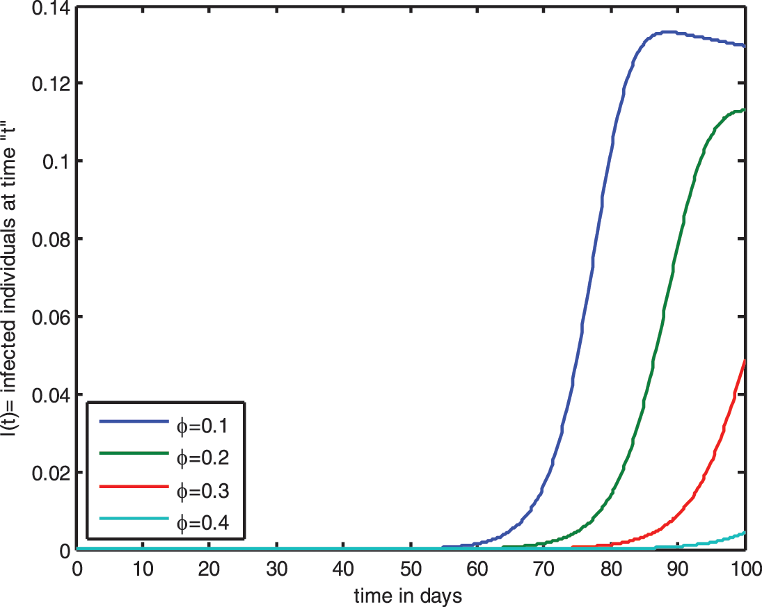
Figure 10: Influence of saturated incidence function for I(t) by varying φ

Figure 11: Influence of saturated incidence function for C(t) by varying φ

Figure 12: Influence of saturated incidence function for A(t) by varying φ

The graph shows that raising the value of φ raises the susceptible population consistently. However, as time passes, the concentration of this population falls. The same phenomenon is observed for HIV infected individuals I(t), HIV infected individuals C(t), HIV infected individuals A(t) in Figs. 10–12. Figs. 13–16 demonstrate the impact of bilinear incidence function for S(t),I(t),C(t), and A(t) populations. From the graph, it is concluded that when the value of parameter ζ (HIV treatment rate) increases, the strength of population also increases. Initially, the susceptible population exhibits almost similar behavior; but, when the value of ζ is increased, a diminution in the population graphing could be noticed. The Fig. 13 displays the impact of HIV treatment rate on healthy population S(t). In the beginning, the concentration level of S(t) increases in uniform succession. However, increasing the HIV treatment rate ζ, a decline is observed in the graph of healthy cells population. Fig. 14 represents a minor change in the concentration of I(t), but after some time, the growth rate of the infected population increases by varying ζ. The similar behavior is stated in the Figs. 15 and 16 for C(t), and A(t), respectively.

Figure 13: Impact of bilinear incidence function for S(t) by varying ζ

Figure 14: Impact of bilinear incidence function ρS for A(t) by varying ζ

Figure 15: Impact of bilinear incidence function for C(t) by varying ζ

Figure 16: Impact of bilinear incidence function ρS for A(t) by varying ζ

Figs. 17–20 demonstrate the dependence of the saturated incidence function ρS1+ε1S on each population one by one. The curves for the susceptible population follow the uniform trajectory initially in Fig. 17. However, after changing the parameter values of ζ from 1.1to1.4, a regular decrease is noticed in the graph. Fig. 18 states that the infected population I(t) is initially in decline, but after varying the HIV treatment rate ζ a regular increase is noticed in the curves. The same behavior is observed in the concentration of the C(t)andA(t) individuals.

Figure 17: Dependence of saturated incidence function ρS1+ε1S for S(t) by varying ζ

Figure 18: Dependence of saturated incidence function for I(t) by varying ζ

Figure 19: Dependences of saturated incidence function for C(t) by varying ζ

Figure 20: Dependences of saturated incidence function for A(t) by varying ζ

5  Mathematical Formulation

Consider an infinite horizontal parallel disk in which incompressible laminar flow of the nanomaterial fluid is examined. The plates are porous and rotating with angular velocity Ω=(0,Ω1,0) along the y−axis. The inspiration of Hall, and radiation is also considered. The nan-fluid model characterizes the Brownian motion and thermophoresis. The framework of the Cartesian coordinate system has been used to determine the problem’s geometry, in which the x−axis is analogous to the platters, the y−axis is the normal, and the z−axis is oblique to the xy-plane. The flow is represented in Fig. 21 as a schematic diagram. When a consistent magnetic flux is pragmatic, the fluid becomes electrically conduct. The lower plate is elongated linearly uw=cx in the x-direction at y=0, while the top plate is at y = h. The lower plate suctions fluid at v=−v0(v0>0 correlates to suction, while v0<0 refers to injection). The imprint of the temperature-thermal conductivity, varied heat generation/absorption mixed with chemical response, and stimulation energy enhance heat and mass transmission. The model equations of nano-fluid stream are [34–39]:

Figure 21: Geometry of the problem

The basic flow equations of Nano liquid are [34–39]:

∂xu~+∂yv~=0,(25)

u~∂xu~+v~∂yu~+2Ω1w~=−1ρ∂xρ+ν(∂xxu~+∂yyu~)+σ1B02ρ(1+m2)(u~−mw~),(26)

u~∂xu~+v~∂yv~=−1ρ∂yρ+ν(∂xxv~+∂yyv~),(27)

u~∂xw~+v~∂yw~−2Ω1u~=ν(∂xxw~+∂yyw~)−σ1B02ρ(1+m2)(mu~+w~),(28)

u~∂xT~+v~∂yT~=1ρCP∂y[k(T)∂yT~]+τ[DB∂yC~∂yT~+DTT~l(∂YT~)2]−1ρcp∂yqr+K(t)uwxvρcp[D(T~w−T~l)f′+H(T~−T~l)],(29)

u~∂xC~+v~∂yC~=DB[(∂xxC~+∂yyC~]+DTT~l(∂xxT~+∂yyT~)−kr2(T~T~l)exp(−EakT~)(30)

With bounded conditions [34,36,37,40]

u~|y=0=uw=cx,v~|y=0=−v0,w~|y=0=0,T~|y=0=T~w,C~|y=0=C~wu~|y=h=0,v~|y=h=0,w~|y=h=0,T~|y=h=T~l,C~|y=h=C~l.(31)

The radioactive heat flux is expressed by the following relation [34,35]:

qr=−43ϱ¯k¯∂yT4,whereT4=4Tl3T−3Tl4(32)

The varying thermal conductivity given in Eq. (29) is explored as [37,39,41,42]:

K=k0(1+d(T−TlTw−Tl))(33)

By using Eqs. (32) and (33), Eq. (29) becomes

u~∂xT~+v~∂yT~=1ρCP∂y[k(t)∂yT~]+τ[DB∂yC~∂yT~+DTT~l(∂YT~)2]+163ϱ¯k¯∂yyT+k0(1+dθ)uwxvρcρ[D(T~w−T~l)f′+H(T~−T~l)],(34)

By proper conversion [34,35,38]

u~=cxf′(η),v~=−chf(η),w~=cxj(η),θ(ζ)=T~−T~lT~w−T~l,(η)=C~−C~lC~w−C~l,ζ=YH.(35)

By using the upstairs conversion Eq. (25) is triflingly equated. However, Eqs. (26)–(28), (30), (31), and (34) yield the system

d4fdη4=Re(dfdηd2fdη2−fd3fdη3)+2α1djdη−Ha2(1+m2)(d2fdη2−mdjdη),(36)

d2jdη2=Re(fdjdη−fdfdηj)−2α1dfdη+Ha2(1+m2)(j+mdfdη),(37)

((1+dθ)+43Rd)Re)d2θdη2=−Pr(fdθdη+Re(Nbdθdηdϕdη+Nt(dθdη)2))−(1+dθ)(Ddfdη+Hdθdη)−Red(dθdη)2,(38)

d2dη2=−NtNbd2θdη2+Sc(δ(1+αθ)nexp(−E(1+αθ))−f.Redϕdη).(39)

The boundary constraints gross the form:

Lower plate:dfdη(0)=1,f(0)=K,j(0)=0,θ(0)=1,ϕ(0)=1,

Upper plate:dfdη(1)=0,f(1)=0,j(1)=0,θ(1)=0,ϕ(1)=0.(40)

The physical quantities of interest are as follows:

Cf,lower=μρuw2∂yu|y=0(41)

Cf,upper=μρuw2∂yu|y=h(42)

Nulower=hQwk0(Tw−Tl),Qw=−k(t)∂yT+qr|y=0(43)

Nuupper=hQwk0(Tw−Tl),Qw=−k(t)∂yT+qr|y=h(44)

Shlower=hQmDB(Cw−Cl),Qm=−DB∂yC|y=0(45)

Shlower=hQmDB(Cw−Cl),Qm=−DB∂yC|y=h.(46)

Using Eqs. (35), (41)–(46) are transformed into

(RehCf)flower=d2fdη2|ζ=0,(RehCf)upper=d2fdη2|η=1(47)

(Nu)lower=−(1+(43).Rd1+dθ)dθdη|η=0,(Nu)upper=−(1+(43).Rd1+dθ)dθdη|η=1(48)

(Sh)lower=−dφdη|η=0,(Sh)upper=−dφdη|η=1.(49)

5.1 Numerical Solutions

This segment is devoted to enclosing a well-known Galerkin scheme to handle the aforementioned nonlinear problems. For the validity of the obtained solution, we compared the present solution with those exist in the published literature. Table 3 provides a comparative analysis of the current study with Tlili et al. [37]. There is a significant correlation between the outcomes.

6  Conclusions

In this paper, we considered the HIV infection model, which consists of four nonlinear ordinary differential equations. We applied an innovative numerical approach known as the continuous Galerkin-Petrov scheme to determine the solution of the model. In addition, we analyzed the dynamics of HIV-infected model with a different incidence rate. Assessed the effects of various clinical parameters on the dynamical behavior of distinct compartments. In the suggested model, we included two types of incidence functions (bilinear and saturated incidence functions) in order to observe visually distinctive fluctuations. By varying the values of various parameters, we observed the periodic rise and fall of the curves of various populations. The bilinear incidence function and the saturated incidence function initially exhibit identical dynamical behavior, as indicated in the illustrations. Nevertheless, with time, various graphical representations evolve. The aforementioned results highlight the importance for mathematical modelling of HIV infection. This will be performed to analyze the population dynamics of CD4+T-cells in the existence and exclusion of HIV, which will be beneficial in identifying clinical AIDS manifestations and in halting the epidemic. It enables physicians with enough information to minimize the viral burden of the disease. The aforementioned approach was employed to investigate a mathematical model for nano-material fluid flow between two analogous infinite disks. The findings are validated through comparison toward those reported in the literature.

Future Recommendations:

It is a well-known observation that fractional analysis has increasingly become a prominent research area. It has been demonstrated that fractional calculus is especially beneficial for imitating a number of legitimate situations. Employing fractional order derivatives and integrals, researchers have evaluated infectious maladies such as COVID-19, HIV, AIDS, and others. The future challenge will involve assessing the quantitative and qualitative aspects of our concept with various fractional order derivatives.

Acknowledgement: The authors would like to thank the editor and anonymous reviewers.

Funding Statement: The authors received no specific funding for this study.

Conflicts of Interest: The authors declare that they have no conflicts of interest to report regarding the present study.

References

1. Mehdi, L. E., Mahrouf, M., Maziane, M., Silva, J., Torres, D. F. M. et al. (2019). A mimimal HIV/AIDS infection model with general incidence and application to Morocco data. Statistics, Optimization & Information Computing, 7, 1–15. [Google Scholar]
2. Corbett, E. L., Watt, C. J., Walker, N., Maher, D., Williams, B. G. et al. (2003). The growing burden of tuberculosis: Global trends and interactions with the HIV epidemic. Archives of Internal Medicine, 163(9), 1009–1021. DOI 10.1001/archinte.163.9.1009. [Google Scholar] [CrossRef]
3. Surur, A. S., Teni, F. S., Wale, W., Ayalew, Y., Tesfaye, B. (2017). Health related quality of life of HIV/AIDS patients on highly active anti-retroviral therapy at a university referral hospital in Ethiopia. BMC Health Services Research, 17(1), 1–8. [Google Scholar]
4. Mannheimer, S. B., Matts, J., Telzak, E., Chesney, M., Child, C. et al. (2005). Quality of life in HIV-infected individuals receiving antiretroviral therapy is related to adherence. AIDS Care, 17(1), 10–22. DOI 10.1080/09540120412331305098. [Google Scholar] [CrossRef]
5. Chávez, J. P., Gürbüz, B., Pinto, C. M. (2019). The effect of aggressive chemotherapy in a model for HIV/AIDS-cancer dynamics. Communications in Nonlinear Science and Numerical Simulation, 75, 109–120. DOI 10.1016/j.cnsns.2019.03.021. [Google Scholar] [CrossRef]
6. Ammassari, A., Murri, R., Pezzotti, P., Trotta, M. P., Ravasio, L. et al. (2001). Self-reported symptoms and medication side effects influence adherence to highly active antiretroviral therapy in persons with HIV infection. JAIDS Journal of Acquired Immune Deficiency Syndromes, 28(5), 445–449. DOI 10.1097/00042560-200112150-00006. [Google Scholar] [CrossRef]
7. Naresh, R., Tripathi, A., Sharma, D. (2011). A nonlinear HIV/AIDS model with contact tracing. Applied Mathematics and Computation, 217(23), 9575–9591. DOI 10.1016/j.amc.2011.04.033. [Google Scholar] [CrossRef]
8. Nyabadza, F., Mukandavire, Z. (2011). Modelling HIV/AIDS in the presence of an HIV testing and screening campaign. Journal of Theoretical Biology, 280(1), 167–179. DOI 10.1016/j.jtbi.2011.04.021. [Google Scholar] [CrossRef]
9. Mushanyu, J. (2020). A note on the impact of late diagnosis on HIV/AIDS dynamics: A mathematical modelling approach. BMC Research Notes, 13(1), 1–8. DOI 10.1186/s13104-020-05179-y. [Google Scholar] [CrossRef]
10. Ullah, S., Khan, M. A. (2020). Modeling the impact of non-pharmaceutical interventions on the dynamics of novel coronavirus with optimal control analysis with a case study. Chaos, Solitons & Fractals, 139, 110075. DOI 10.1016/j.chaos.2020.110075. [Google Scholar] [CrossRef]
11. Geffen, N., Welte, A. (2018). Modelling the human immunodeficiency virus (HIV) epidemic: A review of the substance and role of models in South Africa. Southern African Journal of HIV Medicine, 19(1). DOI 10.4102/sajhivmed.v19i1.756. [Google Scholar] [CrossRef]
12. Alrabaiah, H., Safi, M. A., DarAssi, M. H., Al-Hdaibat, B., Ullah, S. et al. (2020). Optimal control analysis of hepatitis B virus with treatment and vaccination. Results in Physics, 19, 103599. DOI 10.1016/j.rinp.2020.103599. [Google Scholar] [CrossRef]
13. Yüzbaşı, Ş., Karaçayır, M. (2017). An exponential galerkin method for solutions of HIV infection model of CD4+T-cells. Computational Biology and Chemistry, 67, 205–212. DOI 10.1016/j.compbiolchem.2016.12.006. [Google Scholar] [CrossRef]
14. Sohaib, M. (2020). Mathematical modeling and numerical simulation of HIV infection model. Results in Applied Mathematics, 7, 100118. DOI 10.1016/j.rinam.2020.100118. [Google Scholar] [CrossRef]
15. Seatlhodi, T. (2015). Mathematical modelling of HIV/AIDS with recruitment of infected (Dissertation). University of the Western Cape, Department of Mathematics and Applied Mathematics, University of the Western Cape, South Africa. [Google Scholar]
16. Wang, X., Wang, W., Li, Y. (2021). Global stability of switched HIV/AIDS models with drug treatment involving caputo-fractional derivatives. Discrete Dynamics in Nature and Society, 2021. DOI 10.1155/2021/6613171. [Google Scholar] [CrossRef]
17. Rihan, F. A., Al-Mdallal, Q. M., AlSakaji, H. J., Hashish, A. (2019). A fractional-order epidemic model with time-delay and nonlinear incidence rate. Chaos, Solitons & Fractals, 126, 97–105. DOI 10.1016/j.chaos.2019.05.039. [Google Scholar] [CrossRef]
18. Parand, K., Kalantari, Z., Delkhosh, M. (2018). Quasilinearization-lagrangian method to solve the HIV infection model of CD4 $$^+$$+ T cells. SeMA Journal, 75(2), 271–283. DOI 10.1007/s40324-017-0133-1. [Google Scholar] [CrossRef]
19. Ji, C., Jiang, D. (2014). Threshold behaviour of a stochastic SIR model. Applied Mathematical Modelling, 38(21–22), 5067–5079. DOI 10.1016/j.apm.2014.03.037. [Google Scholar] [CrossRef]
20. Kermack, W. O., McKendrick, A. G. (1927). A contribution to the mathematical theory of epidemics. Proceedings of the Royal Society of London Series A, Containing Papers of a Mathematical and Physical Character, 115(772), 700–721. [Google Scholar]
21. Liu, X., Yang, L. (2012). Stability analysis of an SEIQV epidemic model with saturated incidence rate. Nonlinear Analysis: Real World Applications, 13(6), 2671–2679. DOI 10.1016/j.nonrwa.2012.03.010. [Google Scholar] [CrossRef]
22. Attaullah, J. M., Alyobi, S., Yassen, M. F., Weera, W. (2023). A higher order galerkin time discretization scheme for the novel mathematical model of COVID-19. AIMS Mathematics, 8(2), 3763–3790. DOI 10.3934/math.2023188. [Google Scholar] [CrossRef]
23. Ngina, P., Mbogo, R. W., Luboobi, L. S. (2017). The in vivo dynamics of HIV infection with the influence of cytotoxic t lymphocyte cells. International Scholarly Research Notices, 2017. DOI 10.1155/2017/2124789. [Google Scholar] [CrossRef]
24. Ayele, T. K., Goufo, E. F. D., Mugisha, S. (2021). Mathematical modeling of HIV/AIDS with optimal control: A case study in Ethiopia. Results in Physics, 26, 104263. [Google Scholar]
25. Tufail Khan, M., Alyobi, S., Yassen, M. F., Prathumwan, D. (2022). A computational approach to a model for HIV and the immune system interaction. Axioms, 11(10), 578. DOI 10.3390/axioms11100578. [Google Scholar] [CrossRef]
26. Attaullah, Y. Ş., Alyobi, S., Yassen, M. F., Weera, W. (2022). A higher-order galerkin time discretization and numerical comparisons for two models of HIV infection. Computational and Mathematical Methods in Medicine, 2022. DOI 10.1155/2022/3599827. [Google Scholar] [CrossRef]
27. Hussain, S., Schieweck, F., Turek, S. (2011). Higher order galerkin time discretizations and fast multigrid solvers for the heat equation. 19(1), 41–61. DOI 10.1515/jnum.2011.003. [Google Scholar] [CrossRef]
28. Attaullah, R. D., Weera, W. (2022). Galerkin time discretization scheme for the transmission dynamics of HIV infection with non-linear supply rate. Journal: AIMS Mathematics, (6), 11292–11310. DOI 10.3934/math.2022630. [Google Scholar] [CrossRef]
29. Attaullah, R. J. (2020). Solution of the HIV infection model with full logistic proliferation and variable source term using galerkin scheme. Matrix Science Mathematic, 4(2), 37–43. [Google Scholar]
30. Attaullah, J. R., Yüzbaşı, Ş. (2021). Dynamical behavior of HIV infection with the influence of variable source term through galerkin method. Chaos, Solitons & Fractals, 152, 111429. DOI 10.1016/j.chaos.2021.111429. [Google Scholar] [CrossRef]
31. Attaullah, A. S., Yassen, M. F. (2022). A study on the transmission and dynamical behavior of an HIV/AIDS epidemic model with a cure rate. AIMS Mathematics, 7(9), 17507–17528. DOI 10.3934/math.2022965. [Google Scholar] [CrossRef]
32. Sabir, Z., Umar, M., Asif, M., Baleanu, D. (2021). Numerical solutions of a novel designed prevention class in the HIV nonlinear model. Computer Modeling in Engineering & Sciences, 129(1), 227–35. DOI 10.32604/cmes.2021.016611. [Google Scholar] [CrossRef]
33. Amin, R., Yüzbası, Ş., Nazir, S. (2022). Efficient numerical scheme for the solution of HIV infection CD4+T-cells using haar wavelet technique. Computer Modeling in Engineering & Sciences, 131(2), 639–653. DOI 10.32604/cmes.2022.019154. [Google Scholar] [CrossRef]
34. Nadeem, S., Tumreen, M., Ishtiaq, B., Abbas, N., Shatanawi, W. (2022). Second-grade nanofluid flow above a vertical slandering Riga surface with double diffusion model. International Journal of Modern Physics B, 36(32), 2250237. DOI 10.1142/S021797922250237X. [Google Scholar] [CrossRef]
35. Nadeem, S., Ishtiaq, B., Almutairi, S., Ghazwani, H. A. (2022). Impact of Cattaneo–Christov double diffusion on 3D stagnation point axisymmetric flow of second-grade nanofluid towards a Riga plate. International Journal of Modern Physics B, 234205. DOI 10.1142/S0217979222502058. [Google Scholar] [CrossRef]
36. Ishtiaq, B., Zidan, A. M., Nadeem, S., Alaoui, M. K. (2022). Analysis of entropy generation in the nonlinear thermal radiative micropolar nanofluid flow towards a stagnation point with catalytic effects. Physica Scripta, 97(8), 085204. DOI 10.1088/1402-4896/ac79d7. [Google Scholar] [CrossRef]
37. Tlili, I., Hamadneh, N. N., Khan, W. A., Atawneh, S. (2018). Thermodynamic analysis of MHD couette-poiseuille flow of water-based nano fluids in a rotating channel with radiation and hall effects. Journal of Thermal Analysis and Calorimetry, 132(3), 1899–1912. DOI 10.1007/s10973-018-7066-5. [Google Scholar] [CrossRef]
38. Tripathi, R., Seth, G. S., Mishra, M. K. (2017). Double diffusive flow of a hydro magnetic nano fluid in a rotating channel with hall effect and viscous dissipation: Active and passive control of nanoparticles. Advanced Powder Technology, 28(10), 470–481. [Google Scholar]
39. Ramzan, M., Gul, H., Kadry, S. (2019). Onset of Cattaneo-Christov heat flux and thermal stratification in ethylene-glycol based nano fluid flow containing carbon nanotubes in a rotating frame. IEEE Acces, (s7), 146190–146197. DOI 10.1109/Access.6287639. [Google Scholar] [CrossRef]
40. Fuzhang, W., Akhtar, S., Nadeem, S., El-Shafay, A. S. (2022). Mathematical computations for the physiological flow of casson fluid in a vertical elliptic duct with ciliated heated wavy walls. Waves in Random and Complex Media. DOI 10.1080/17455030.2022.2072973. [Google Scholar] [CrossRef]
41. Attia, H. A. (2008). Unsteady hydro magnetic couette flow of dusty fluid with temperature dependent viscosity and thermal conductivity. International Journal of Non-Linear Mechanics, 43(8), 707–715. DOI 10.1016/j.ijnonlinmec.2008.03.007. [Google Scholar] [CrossRef]
42. Hayat, T., Farooq, S., Ahmad, B., Alsaedi, A. (2018). Consequences of variable thermal conductivity and activation energy on peristalsis in curved configuration. Journal of Molecular Liquids, 263, 258–267. DOI 10.1016/j.molliq.2018.04.109. [Google Scholar] [CrossRef]
Cite This Article
Copyright © 2023 The Author(s). Published by Tech Science Press.
This work is licensed under a Creative Commons Attribution 4.0 International License , which permits unrestricted use, distribution, and reproduction in any medium, provided the original work is properly cited.
Downloads
Citation Tools