Theory and Semi-Analytical Study of Micropolar Fluid Dynamics through a Porous Channel

1  Introduction

The Navier-Stokes model of classical hydrodynamics has some limitations. It has no bearing on the fluid’s microstructure. The best explanation for the hypothesis of microstructure fluid is micropolar fluid. Eringen [1] proposed the theory of micropolar fluid for the first time in 1966, When he was working on various classes of fluid that demonstrated specific microscopic effects coming from micro-motion of the fluid elements. It consists of a non-Newtonian fluid and a combination of tiny hard particles orientated randomly. To put it another way, a fluid whose molecules may spin independently of the flow of the fluid stream. Micropolar fluid flow has a wide range of applications in industries such as chemistry, biomedicine, and medicine. It may also be used on natural materials like sandstone, capillary blood system of the lungs and limestone. Researchers have recently concentrated their efforts on micropolar fluids and related phenomena [2–7]. Mass and heat transport in the porous channel and material media get much attention of researchers, because of many applications such as thermal storage of power, geothermal recovery of energy, oil extraction, collector of solar power, process of electro chemical, grain storage, regenerative heat and flow through filtering device [8–16].

The majority of scientific issues, particularly mass transfer and certain heat transfer, as well as other phenomena in our environment, are nonlinear. Nonlinear DEs describe these nonlinear issues and occurrences. Many mathematical models of physical systems give rise to nonlinear DEs. As a result, some of them can be solved numerically while others may be solved analytically using perturbation techniques, spectrum approaches and decompositions, etc. However, there are some nonlinear situations that do not have a perturbation quantity like HAM [17,18], HPM [19], OHAM [20] and ADM [21]. Similarly some further updated versions of the aforementioned methods have been applied to study various problems in fluid mechanics, we refer few as [22–25].

The differential transform technique (DT) is a semi-analytical approach for solving nonlinear and linear differential equations. DTM core concept was first proposed by Ayaz [26] in 1986 in electrical circuit analysis for handling linear and nonlinear problems. The DTM is an iterative method for obtaining analytical Taylor series solutions to nonlinear and linear differential equations. However, it is not the same as the Taylor series approach. Because of the high order derivatives, the Taylors series approach is computationally difficult. This approach has the benefit of being able to be used directly to nonlinear and linear DEs without the need for linearization or discretization. As a result, the discretization defect has no effect on DTM.

The DTM was utilized by Hatami et al. [27] to solve PDEs. The similar approach was also utilized by Jang et al. [28], for the solution of a system of DEs. To demonstrate the correctness and simplicity of this technique, Hatami et al. [29] adapted it for the solution of a coupled system of nonlinear DEs. The two-dimensional DTM was presented by Sheikholeslami et al. [30], for the solution of PDEs. This approach for solving non-Newtonian flow in an axi-symmetric porous channel was presented by Sepasgozar et al. [31]. By taking into account thermophoresis and the Brownian effect, Bejawada et al. [32] have expanded their work on DTM to the solution of nano-fluid flow between parallel plates.

The major goal of this research is to use DTM to solve nonlinear DEs that are two-dimensional laminar, steady flow and incompressible, that are governed by micropolar flow in a porous channel. DTM may also be considered as a powerful tool for solving nonlinear systems, modeling ODEs and PDEs, and solving integral equations. We compare our findings to those obtained using a numerical approach such as RK4. We also evaluate the influence of factors like the bouncy ratio, spin gradient viscosity parameter, Reynolds number and related parameters when calculating the flow model equations. Using mathematica, the various behavior of these parameters is illustrated on graphs.

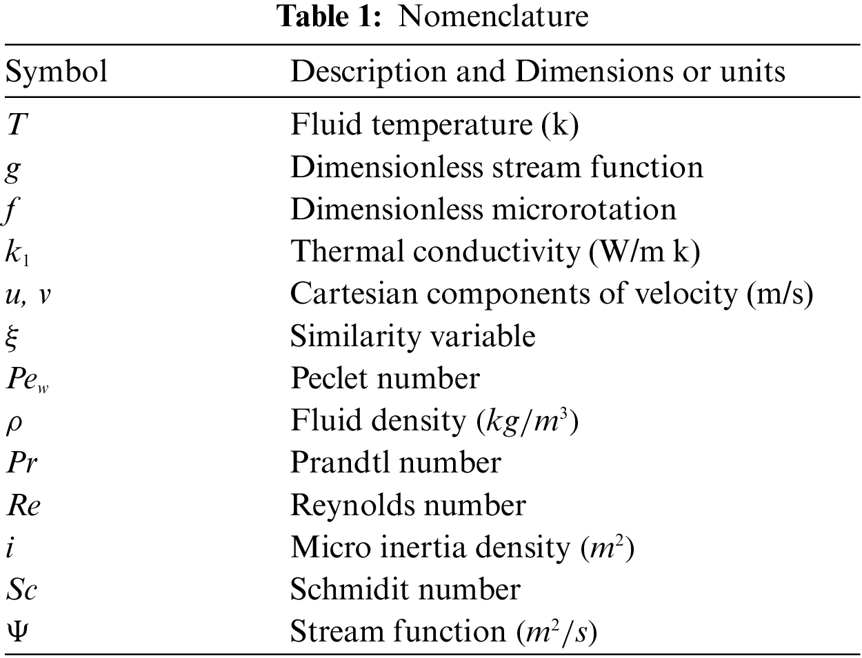
Here we remark that the DTM is a powerful method in handling many weakly and strongly nonlinear problems. The computation is easy and the method does not need any kinds of axillary parameters to control the procedure like HAM. Also the procedure does not required any prior discretization or collocation like other numerical methods need. The method is rapidly convergent and this phenomenon has been proved in many articles. We refer in this regards some papers as [33–35]. Here we give a Nomenclature in Table 1.

2  Mathematical Formulation of the Flow Problem

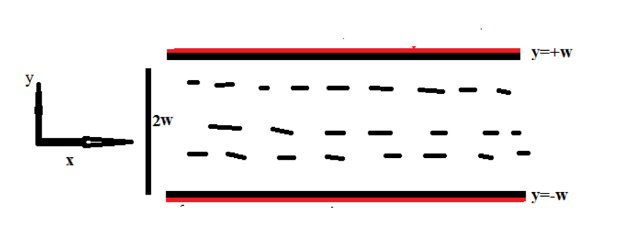
We address laminar incompressible, steady, two-dimensional micropolar flow in a porous channel in this formulation. In this formulation, we consider steady, laminar incompressible and two-dimensional micropolar flow in a porous channel. The flow uniformly injected or moved with speed s. The channel walls placed at y=±h and parallel to x−axis, 2h is the separated distance of channel walls. The flow was evenly injected or transported at a constant s speed. 2w is the separated distance of channel walls, which are located at y=±w and parallel to the x−axis. The governing equations of the flow in invariant form [36] is given as

{∂p∂t+∇(pv→)=0,ρ(Dv→Dt)=−∇p+(μ+k)∇2v→+k∇N,ρ(DNDt)=−ki(2N+∇×v→)+vsi∇2N.(1)

By including temperature effect in (1), the following model [37] was formulated as

∂p∂t+∇(pv→)=0,(2)

ρ(Dv→Dt)=−∇p+(μ+k)∇2v→+k∇N,(3)

ρ(DNDt)=−kj(2N+∇×v→)+vsi∇2N.(4)

ρCp(v→⋅∇T)=k∇2T.(5)

In Fig. 1, we provide physical description of the considered model. Since the flow is in 2-dimension, so the above equation in component form can be written as

∂u∂x+∂v∂y=0,(6)

ρ(u∂u∂x+v∂u∂y)=−∂p∂x+(μ+r)(∂2u∂x2+∂2u∂y2)+k∂𝒜∂y,(7)

ρ(u∂v∂x+v∂v∂y)=−∂p∂y+(μ+k)(∂2v∂x2+∂2v∂y2)−k∂𝒜∂x,(8)

ρ(u∂θ∂x+v∂θ∂y)=−ki+(2𝒜+∂u∂y−∂v∂x)+(μsj)(∂2𝒜∂x2+∂2𝒜∂y2),(9)

ρ(u∂T∂x+v∂T∂y)=k1cρ∂2T∂y2.(10)

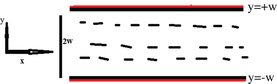
Figure 1: Plot which shows the physical description of the considered problem

Using

y=−w:v=v∘,u=0𝒜=−s∂u∂y|y=−w,y=+w:u=0,v=v0,𝒜=−s∂u∂y|y=+w.(11)

where v0>0 is suction case, and when v0<0 is injective case, and s is boundary parameter. If s=0, then concentrated particle flows where microclimates are unable to rata close to the wall. Next we introduce the following similarity variables:

ξ=yw,ψ=−v0xg(ξ),𝒜=v0xw2f(ξ),θ(ξ)=T−T2T1−T2,T2=T1−Ax,(12)

where A is constant. Further, we use stream functions as

u=∂ψ∂y,v=−∂ψ∂x.(13)

Using (11)–(13), the proposed equations from (6)–(10) are transformed to the following system of nonlinear ordinary differential equations:

(1+𝒜1)giv−𝒜1f″−Re(gg‴+g′g″)=0,(14)

𝒜2f″+𝒜1(g″−2f)−𝒜3Re(gf′−fg′)=0,(15)

θ″+Pewg′θ−Pemgθ′=0,(16)

with boundary conditions as

ξ=−1:g=−1,f=g′=0,θ=1,ξ=−1:g=+1:g′=f=θ=0.(17)

The buoyancy ratio 𝒜, the Peclet number of the diffusion of heat Pew and mass Pem have of fundamental interest. There are two cases for the Reynolds number (Re), if Re>0 corresponding to suction and if Re<0 to injection. Also 𝒜1=kμ,𝒜2=vsμw,𝒜3=iw2,Re=v0wv,Pr=vρcρk1,Pew=PrRe,Pem=ScRe, where Pr stands for Prandtl number and Sc is the generalized Schmidt number. Also 𝒜1 and 𝒜2 are coupling parameter and spin gradient velocity parameter, respectively.

3  Basic Definitions and Operations of DTM

In this section, we define some basic operations and definitions of DTM [15] as given below: The differential transform of function h(ξ) for the nth derivative of the function is define by

H(ξ)=1n![dnh(ξ)dξn]ξ=ξ∘,(18)

where H(n) is the transform function of h(ξ) in the domain “n” at ξ=ξ∘. which also know as T−function or spectrum of h(ξ).

The inverse transformation as define by

h(ξ)=∑n=0∞H(n)(ξ−ξ∘)n.(19)

Combining Eqs. (18) and (19), we get the following result:

h(ξ)=∑n=0∞[dnh(ξ)dξn]ξ=ξ∘(ξ−ξ∘)nn!.(20)

From above Eq. (20), it is clear that the basic concept of DTM is obtain from Taylor’s series expansion, but the procedure does not calculate the derivatives symbolically, relative derivative are evaluate by an iterative method. Which can be obtain from transformation of the given original functions. In case of finite series, where M is the series size, the Eq. (19) can be express as follows:

h(ξ)=∑n=0MH(n)(ξ−ξ∘)n.(21)

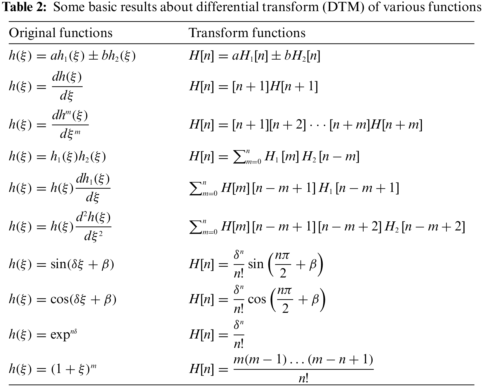
The basic results and operations of DTM which are obtain from Eqs. (19) and (20) are need throughout in this work, which are given below on the Table 2.

4  Computation of Solution for the Obtained ODEs (14)–(16)

Now we apply DTM into governing coupled system of nonlinear ODEs (14)–(16) and boundary conditions (17) as

(1+𝒜1)(n+1)(n+2)(n+3)(n+4)G[n+4]−(𝒜1)(n+1)(n+2)F[n+2]−Re∑m=0nG[n−m](m+1)(m+2)(m+3)G[m+3]−Re∑m=0n(n−m+1)G[n−m+1](m+1)(m+2)G[m+2]=0,(22)

(𝒜2)(n+1)(n+2)F[n+2]+𝒜1(n+1)(n+2)G[n+2]−2𝒜1F[n]−𝒜3Re∑m=0nG[n−m](m+1)F[m+1]+𝒜3Re∑m=0nF[n−m](m+1)G[m+1]=0,(23)

(n+1)(n+2)Θ[n+2]+eh[∑m=0n(m+1)G[m+1](n−m)Θ[n−m]]−eh[∑m=0nG[m](n−m+1)Θ[n−m+1]]=0,(24)

with boundary conditions are

ξ=−1:G[0]=G[1]=0,F[0]=0,Θ[0]=0ξ=+1:G[0]=0,G[1]=−1,F[0]=1,Θ[0]=1,(25)

where G[n], F[n] and Θ[n] are the transformed function of g(ξ), f(ξ) and θ(ξ), respectively, and are given below:

g(ξ)=∑n=0∞G[n]ξn,(26)

f(ξ)=∑n=0∞F[n]ξn.(27)

and

θ(ξ)=∑n=0∞Θ[n]ξn.(28)

Hence, we substituting the value of G[n], F[n] and Θ[n] in Eqs. (26)–(28) to get the series solution of coupled system of nonlinear ODEs.

We consider the following additional boundary conditions which lead the solution of the Eqs. (22)–(24) as

G[0]=α1,G[1]=α2,G[2]=α3,G[3]=α4,F[0]=β1,F[1]=β2,Θ[0]=γ1,Θ[1]=γ2,(29)

where αi(i=1,2,3,4), βi(i=1,2) and γi(i=1,2) are constants which can be determine through the computational software like mathematica. For instance, if 𝒜1=𝒜2=𝒜3=0.5, Peh=Pem=0.3 and Re=0.7, we compute the approximate values of αi(i=1,2,3,4), βi(i=1,2) and γi(i=1,2) as

α1=−0.04567,α2=1.01879,α3=0.056743,α4=−1.02735,β1=0.0123456,β2=−1.02735,γ1=0.78765,γ2=−0.168694(30)

Using the values given in (30), we obtain the required series solution as

g(ξ)=−0.005678+1.01879ξ+0.0345678ξ2−1.02735ξ3−0.0463553ξ4+0.0352885ξ5−0.0023456ξ6−0.00234516ξ7−0.00032145ξ8+⋯,f(ξ)=0.0123456−0.168694ξ−0.66879ξ2+0.733401ξ3+0.055008ξ4−2.12446ξ5−0.00654321ξ6−0.0123789ξ7−0.000453217ξ8+⋯,θ(ξ)=0.78765−0.78768ξ+0.00056789ξ2−0.0000000453ξ3−0.000055008ξ4−0.0065432ξ5−0.000001326ξ6−0.000000089ξ7−0.0000009876ξ8+⋯.(31)

Remark 1. Here we remark that DTM is rapidly convergent procedure. In this regards, various results related to convergence of the mentioned method for ODEs has been given in [33–35].

5  Numerical Simulation and Results and Discussion

In this section, we introduce graphical representation of our results to show accuracy of DTM for the solution of micropolar flow in a porous channel. The Fig. 2 shows the combine graph of function f, g and θ. The Fig. 3 demonstrates the accuracy of DTM for the flow model. Here, we compare our result with the results of RK4 method for the obtained nonlinear Eqs. (14)–(16). We see that our solution has good agreement with the numerical solution obtained by RK4 method. Beside this, we also check the parametric effects which show different effect on the profile of f, g and θ. In Figs. 4–6, we have shown the effect of Re on the profile of f, g and θ by fixing the values of 𝒜i(i=1,2,3). Also, in Figs. 7–9, we have testified the effect of 𝒜i(i=1,2,3) on the profile of f, g and θ by taking the values Re=1. From Figs. 4–9, we see that Re as well as the values of 𝒜i(i=1,2,3) have great effect on the profile of f, g and θ. The effect on the concerned profile can be obviously observed from Figs. 4–9.

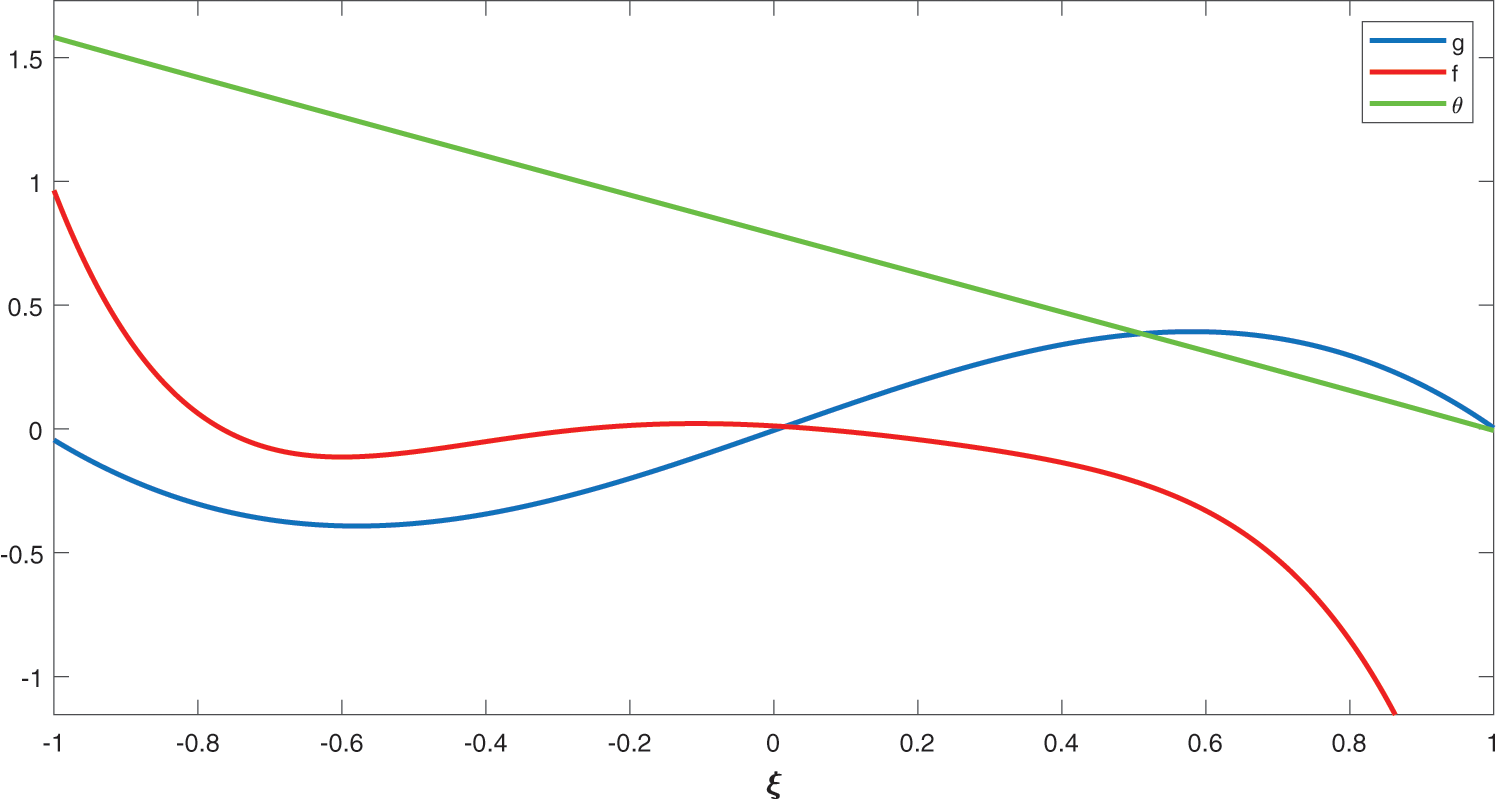
Figure 2: Combine of the profiles of f, g and θ

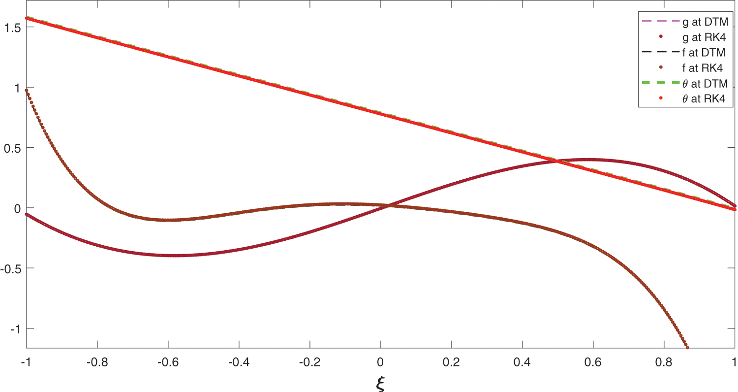
Figure 3: Comparison of 9th-order approximate solation of DTM with RK4 with Re=0.4,Peh=Pem=0.4

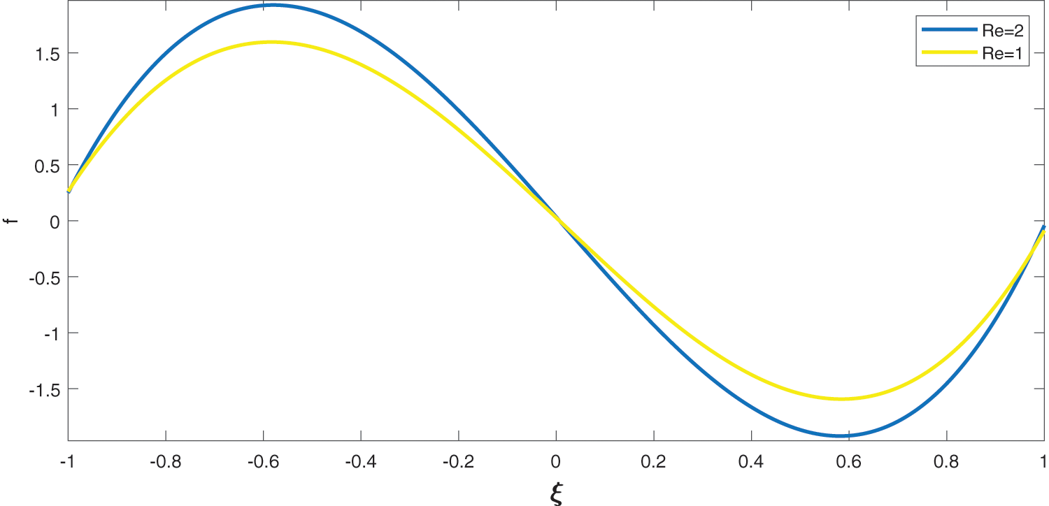
Figure 4: Effect of Re on g with 𝒜1=𝒜2=𝒜3=0.5

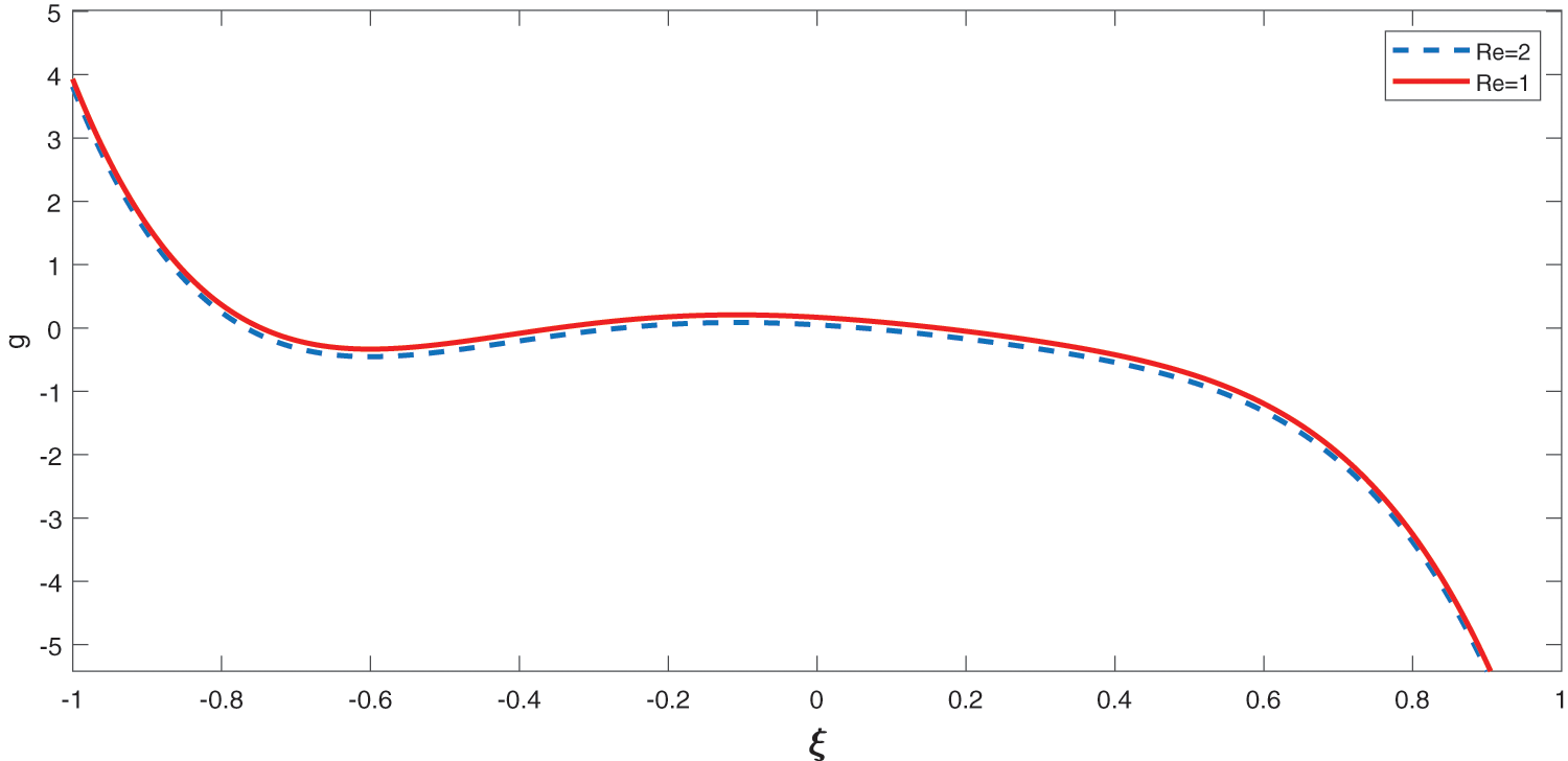
Figure 5: Effect of Re on f with 𝒜1=𝒜2=𝒜3=0.5

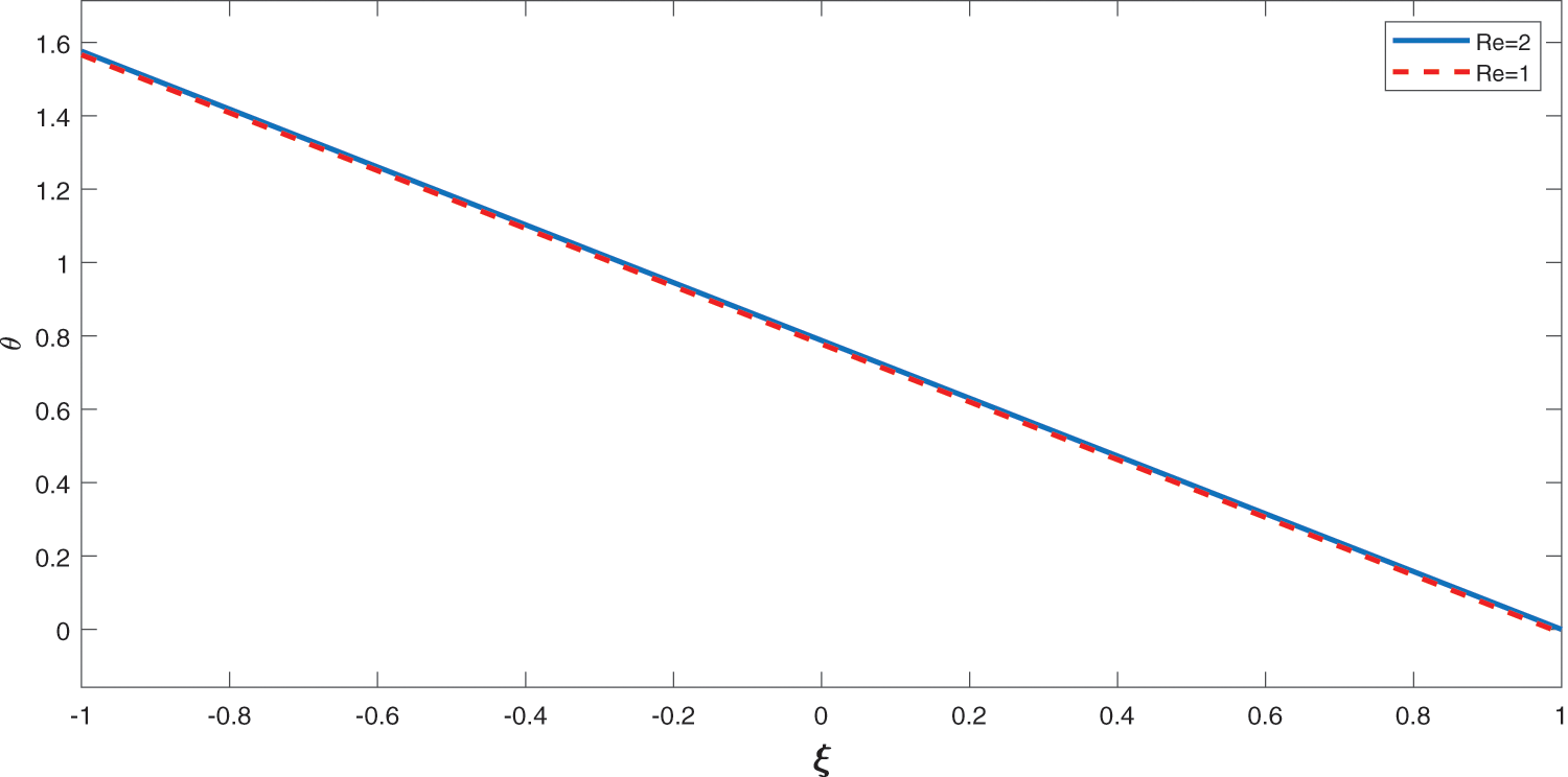
Figure 6: Effect of Re on θ with 𝒜1=𝒜2=𝒜3=0.5

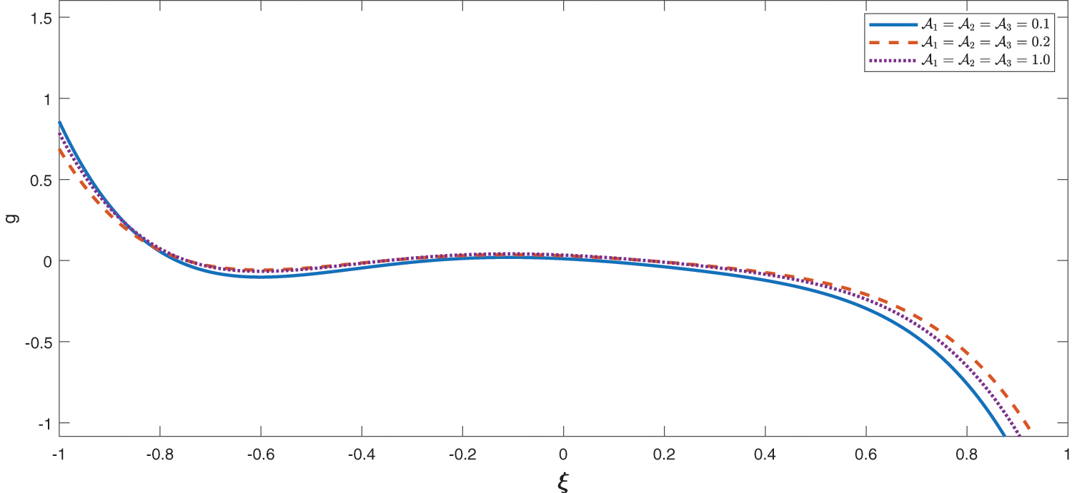
Figure 7: Effect of 𝒜1,𝒜2,𝒜3 on the profile of g with Re=1

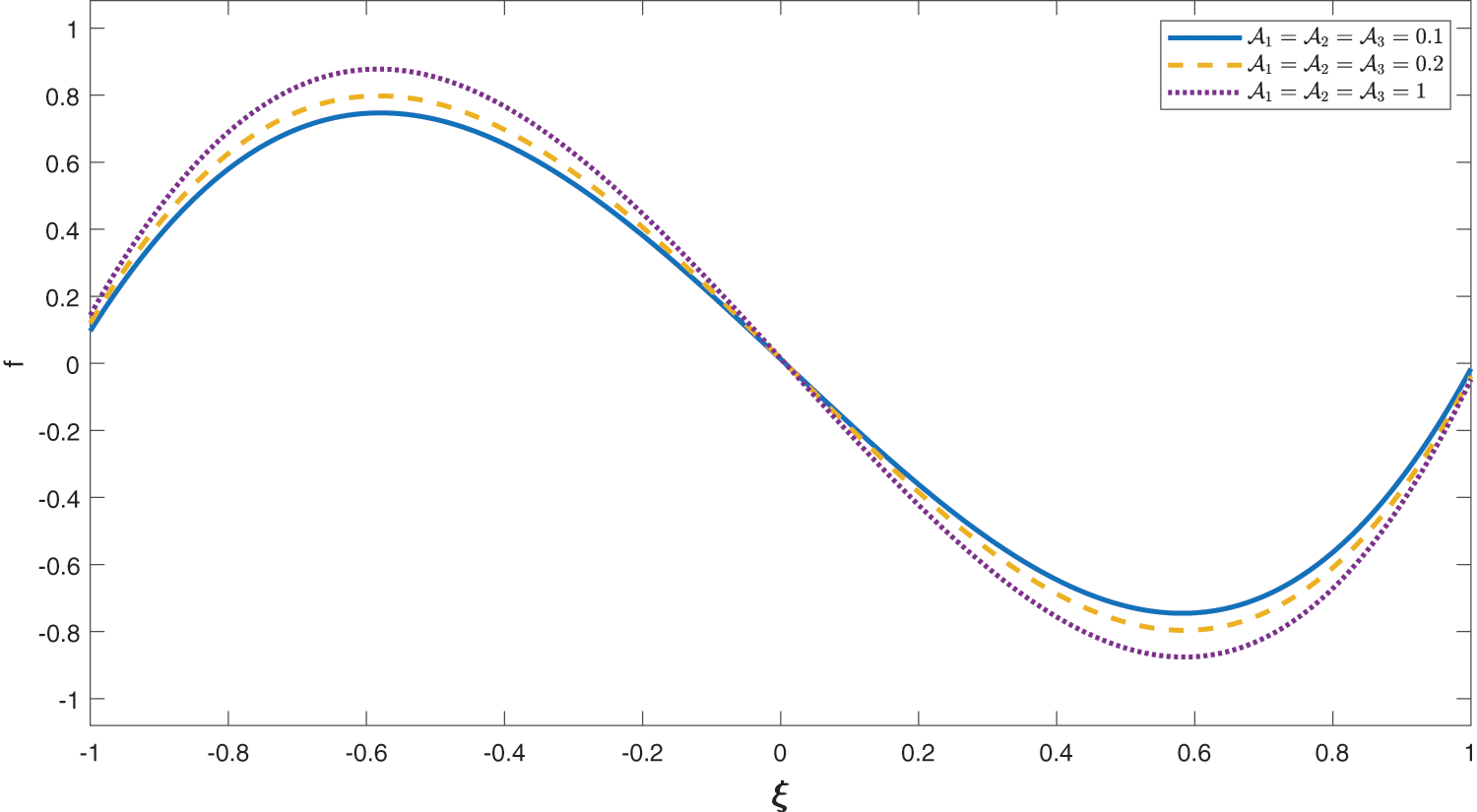
Figure 8: Effect of 𝒜1,𝒜2,𝒜3 on the profile of f with Re=1

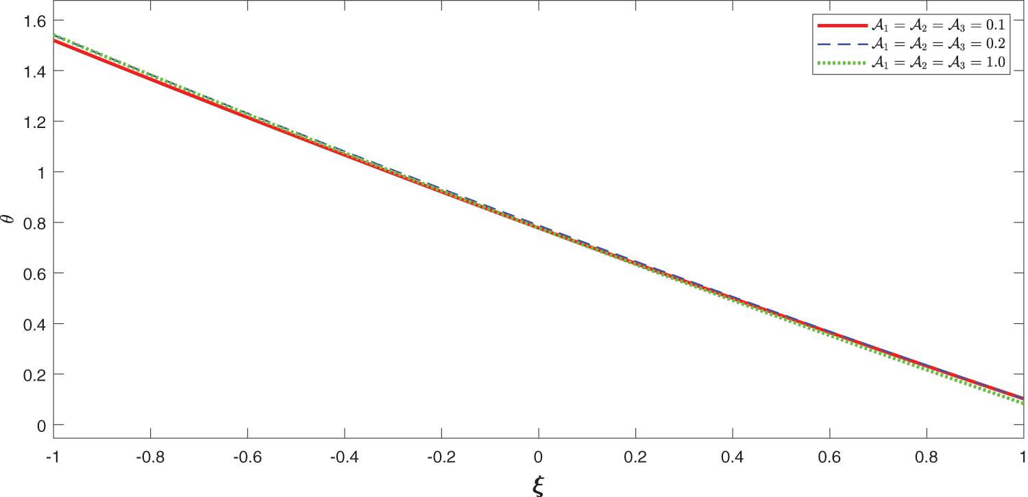
Figure 9: Effect of 𝒜1,𝒜2,𝒜3 on the profile of θ with Re=1

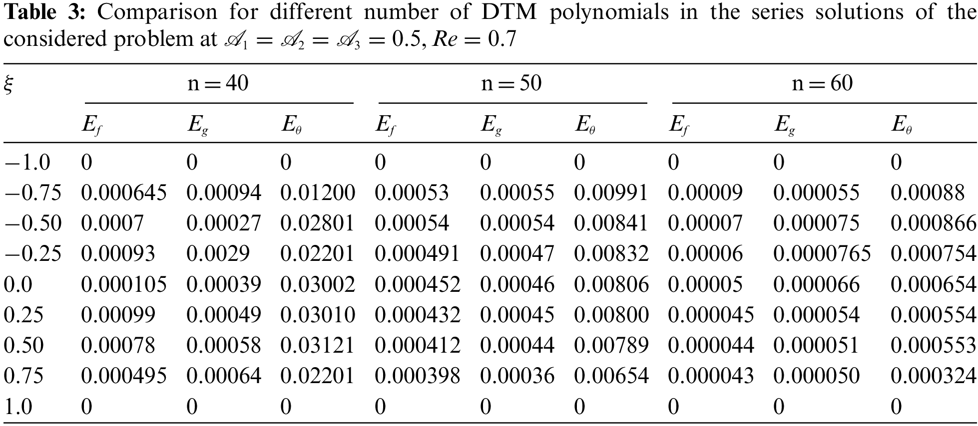
In Table 3, we have computed absolute error of different numbers of polynomials of DTM that are for n=40 polynomials, n=50 and n=60 polynomials. We see that as the numbers of polynomials are increasing, the error is reducing, so we conclude that the more the numbers of DTM polynomials more will be the accuracy and vice versa.

6  Concluding Remarks

We have examined in detail the nature of micropolar flow in porous channels with high mass transfer through the channel wall. The problem has been solved via a sort of analytical method called DTM. Hence we concluded that DTM is the powerful and efficient approach for solving nonlinear ODEs and their systems arising from micropolar flow in porous channel walls. In alternate ways, for this problem, we have compared our results with the famous numerical method RK4, which revealed that our analytical results have a close agreement with the numerical results (see Fig. 3). We have also discussed different parametric effects on the solutions of stream function, velocity profile and temperature of the flow model. The effect of Re and others parameters including 𝒜i(i=1,2,3) have been investigated. The respective effect on the profiles of the mentioned quantities has been presented graphically in Figs. 4–9. Here it should be kept in mind that DTM needs no prior discretization of data nor requires any collocation of data elements. Further, the method is independent of axillary parameters which control the procedure like in Homotopy analysis and perturbation method. Further, the DTM is a rapidly convergent method.

Funding Statement: Princess Nourah bint Abdulrahman University Researchers Supporting Project No. (PNURSP2023R14), Princess Nourah bint Abdulrahman University, Riyadh, Saudi Arabia. Further, authors Aziz Khan, K. Shah and T. Abdeljawad would like to thank Prince Sultan University for the support through the TAS Research Lab.

Author Contributions: All authors contributed equally and significantly in writing this article. All authors read and approved the final manuscript.

Availability of Data and Materials: The data that supports the findings of this study are available within the article.

Conflicts of Interest: The authors declare that they have no known competing financial interests or personal relationships that could have appeared to influence the work reported in this paper.

References

    1. Eringen, A. C. (1966). Theoery of micropolar fluid. Mathematics and Mechanics, 16(1), 1–18. [Google Scholar]

    2. Cheng, C. Y. (2008). Natural convection heat and mass transfer from asphere in micropolar fluid with constant wall temperature and concentration. International Communications in Heat and Mass Transfer, 35(6), 750–755. DOI 10.1016/j.icheatmasstransfer.2008.02.004. [Google Scholar] [CrossRef]

    3. Goud, B. S. (2020). Heat generation/absorption influence on steady stretched permeable surface on MHD flow of a micropolar fluid through a porous medium in the presence of variable suction/injection. International Journal of Thermofluids, 7, 100044. [Google Scholar]

    4. Bejawada, S. G., Reddy, Y. D., Kumar, K. S., Kumar, E. R. (2021). Numerical solution of natural convection on a vertical stretching surface with suction and blowing. International Journal of Heat and Technology, 39, 1469–1474. [Google Scholar]

    5. Yanala, D. R., Mella, A. K., Vempati, S. R., Goud, B. S. (2021). Influence of slip condition on transient laminar flow over an infinite vertical plate with ramped temperature in the presence of chemical reaction and thermal radiation. Heat Transfer, 50(8), 7654–7671. DOI 10.1002/htj.22247. [Google Scholar] [CrossRef]

    6. Bejawada, S. G., Khan, Z. H., Hamid, M. (2021). Heat generation/absorption on MHD flow of a micropolar fluid over a heated stretching surface in the presence of the boundary parameter. Heat Transfer, 50(6), 6129–6147. DOI 10.1002/htj.22165. [Google Scholar] [CrossRef]

    7. Srinivasulu, T., Goud, B. S. (2021). Effect of inclined magnetic field on flow, heat and mass transfer of Williamson nanofluid over a stretching sheet. Case Studies in Thermal Engineering, 23, 100819. DOI 10.1016/j.csite.2020.100819. [Google Scholar] [CrossRef]

    8. Rashidi, M. M., Hayat, T., Keimanesh, T., Yousefian, H. (2012). A study on heat tranfer in a second grad fluid through a porous medium with the modifid differential transform method. Heat Transfer Asian Research, 1(24), 1–12. [Google Scholar]

    9. Hassan, H., Rashid, M. M. (2014). An analytical soluation of micropolar flow in porous channel with mass injection using homotopy analysis method. International Journal of Numerical Methods for Heat & Fluid Flow, 2(24), 419–437. [Google Scholar]

  10. Rashidi, M. M., Abbasbandy, S. (2011). Analytical approximate soluation for heat transfer of a micropolar fluid through a porous medium with radiation. Communications in Nonlinear Science and Numerical Simulation, 16(4), 1874–1889. DOI 10.1016/j.cnsns.2010.08.016. [Google Scholar] [CrossRef]

  11. Inç, M., Khan, H., Baleanu, D., Khan, A. (2018). Modified variational iteration method for straight fins with temperature dependent thermal conductivity. Thermal Science, 22(1), S229–S236. [Google Scholar]

  12. Baleanu, D., Khan, H., Jafari, H., Khan, R. A. (2015). On the exact solution of wave equations on cantor sets. Entropy, 17(9), 6229–6237. DOI 10.3390/e17096229. [Google Scholar] [CrossRef]

  13. Abro, K. A., Atangana, A. (2020). A comparative study of convective fluid motion in rotating cavity via Atangana–Baleanu and Caputo–Fabrizio fractal–fractional differentiations. The European Physical Journal Plus, 135(2), 1–16. [Google Scholar]

  14. Shah, Z., Islam, S., Gul, T., Bonyah, E., Khan, M. A. (2018). The electrical MHD and hall current impact on micropolar nanofluid flow between rotating parallel plates. Results in Physics, 9, 1201–1214. DOI 10.1016/j.rinp.2018.01.064. [Google Scholar] [CrossRef]

  15. Shah, Z., Islam, S., Ayaz, H., Khan, S. (2019). Radiative heat and mass transfer analysis of micropolar nanofluid flow of Casson fluid between two rotating parallel plates with effects of hall current. Journal of Heat Transfer, 141(2), 022401. DOI 10.1115/1.4040415. [Google Scholar] [CrossRef]

  16. Shoaib, M., Raja, M. A. Z., Farhat, I., Shah, Z., Kumam, P. et al. (2022). Soft computing paradigm for Ferrofluid by exponentially stretched surface in the presence of magnetic dipole and heat transfer. Alexandria Engineering Journal, 61(2), 1607–1623. DOI 10.1016/j.aej.2021.06.060. [Google Scholar] [CrossRef]

  17. Sheikholeslami, M., Ellahi, R., Ashorynejad, H. R., Domairry, G., Hayat, T. (2014). Effects of heat transfer in flow of nanofluids over a permeable stretching wall in a porous medium. Journal of Computational and Theoretical Nanoscience, 11(2), 486–496. DOI 10.1166/jctn.2014.3384. [Google Scholar] [CrossRef]

  18. Sheikholeslami, M., Ganji, D. D., Rokni, H. B. (2013). Nanofluid flow in a semi-porous channel in the presence of uniform magnetics field. Flow between parallel plates. International Journal of Engineering, 26(6), 653–662. [Google Scholar]

  19. Sheikholeslami, M., Ganji, D. D., Ashorynejad, H. R. (2013). Investigation of squeezing unsteady nanofluid flow using ADM. Powder Technology, 239, 259–265. DOI 10.1016/j.powtec.2013.02.006. [Google Scholar] [CrossRef]

  20. Zhou, J. K. (1986). Differentail transformation and its applications for electrical circuits, pp. 1279–1289. Wuhan, China: Huarjung University Press. [Google Scholar]

  21. Türkyilmazoglu, M. (2019). Accelerating the convergence of adomian decomposition method (ADM). Journal of Computational Science, 31, 54–59. DOI 10.1016/j.jocs.2018.12.014. [Google Scholar] [CrossRef]

  22. Türkyilmazoglu, M. (2018). A reliable convergent adomian decomposition method for heat transfer through extended surfaces. International Journal of Numerical Methods for Heat & Fluid Flow, 28(11), 2551–2566. DOI 10.1108/HFF-01-2018-0003. [Google Scholar] [CrossRef]

  23. Turkyilmazoglu, M. (2015). Is homotopy perturbation method the traditional Taylor series expansion. Hacettepe Journal of Mathematics and Statistics, 44(3), 651–657. DOI 10.15672/HJMS.2015449416. [Google Scholar] [CrossRef]

  24. Türkyilmazoglu, M. (2019). Equivalence of ratio and residual approaches in the homotopy analysis method and some applications in nonlinear science and engineering. Computer Modeling in Engineering & Sciences, 120(1), 63–81. DOI 10.32604/cmes.2019.06858. [Google Scholar] [CrossRef]

  25. Türkyilmazoglu, M. (2021). Nonlinear problems via a convergence accelerated decomposition method of Adomian. Computer Modeling in Engineering & Sciences, 127(1), 1–22. DOI 10.32604/cmes.2021.012595. [Google Scholar] [CrossRef]

  26. Ayaz, F. (2004). Solution of the system of differential equation by differentail trasform method. Applied Mathematics and Computation, 147(2), 547–567. DOI 10.1016/S0096-3003(02)00794-4. [Google Scholar] [CrossRef]

  27. Hatami, M., Jing, D. (2016). Differential transform method for Newtonian and non-Newtonian flow analysis. Alexandria Engineering Journal, 55(2), 731–739. DOI 10.1016/j.aej.2016.01.003. [Google Scholar] [CrossRef]

  28. Jang, M. J., Chen, C. L., Liue, Y. C. (2001). Two-dimensional differential transform for partial differential equation. Applied Mathematics and Computation, 121(3), 261–270. [Google Scholar]

  29. Hatami, M., Jing, D. (2017). Optimization of wavy direct absorber solar collector (WDASC) using Al2O3-water nanofluid and RSM analysis. Applied Thermal Engineering, 121, 1040–1050. DOI 10.1016/j.aej.2016.01.003. [Google Scholar] [CrossRef]

  30. Sheikholeslami, M., Rashidi, M. M., Al Saad, D. M., Firouzi, F., Rokni, H. B. et al. (2016). Steady nanofluid flow between parallel plates considering thermophoresis and Brownian effects. Journal of King Saud University-Science, 28(4), 380–389. DOI 10.1016/j.jksus.2015.06.003. [Google Scholar] [CrossRef]

  31. Sepasgozar, S., Faraji, M., Valipour, P. (2017). Application of differential transformation method (DTM) for heat and mass transfer in a porous channel. Propulsion and Power Research, 6(1), 41–48. DOI 10.1016/j.jppr.2017.01.001. [Google Scholar] [CrossRef]

  32. Bejawada, S. G., Nandeppanavar, M. M. (2022). Effect of thermal radiation on magnetohydrodynamics heat transfer micropolar fluid flow over a vertical moving porous plate. Experimental and Computational Multiphase Flow, 1–10. DOI 10.1007/s42757-021-0131-5. [Google Scholar] [CrossRef]

  33. Oke, A. S. (2017). Convergence of differential transform method for ordinary differential equations. Journal of Advances in Mathematics and Computer Science, 24(6), 1–17. [Google Scholar]

  34. Odibat, Z. M., Kumar, S., Shawagfeh, N., Alsaedi, A., Hayat, T. (2017). A study on the convergence conditions of generalized differential transform method. Mathematical Methods in the Applied Sciences, 40(1), 40–48. DOI 10.1002/mma.3961. [Google Scholar] [CrossRef]

  35. Moosavi Noori, S. R., Taghizadeh, N. (2021). Study of convergence of reduced differential transform method for different classes of differential equations. International Journal of Differential Equations, 2021, 6696414. [Google Scholar]

  36. Lukaszewicz, G. (1999). Micropolar fluids: Theory and applications. New York: Springer Science & Business Media. [Google Scholar]

  37. Abdul Latiff, N. A., Uddin, M. J., Bég, O. A., Ismail, A. I. (2016). Unsteady forced bioconvection slip flow of a micropolar nanofluid from a stretching/shrinking sheet. Proceedings of the Institution of Mechanical Engineers, Part N: Journal of Nanomaterials, Nanoengineering and Nanosystems, 230(4), 177–187. [Google Scholar]