Metric Identification of Vertices in Polygonal Cacti

1  Introduction

The metric dimension is used in a variety of scientific disciplines, including chemical graph theory and computer networking. A technique for finding a vertex’s precise location or position in a network is called localization. In a work environment, localization is used when a computer sends a printing command to help locate nearby printers, broken equipment, network intruders, illegal or unauthorised connections, and wandering robots. The localization of a network is a difficult, expensive, time-consuming, and arduous procedure. The minimum number of vertices (the metric dimension of a graph representing the network) is picked in such a way that, with the aid of selected vertices, the location of the required vertex may be identified by its distinctive representation.

In robotic engineering, there is no concept of direction and no visibility on a polygonal type planar surface/mesh. So handling the navigation of a robot (a navigation agent) from point to point is a crucial task, which can be done quickly with the help of distinctively labelled landmarks. These landmarks help the robot locate itself on the surface (or graph). The visual detection of a landmark sends information to the robot about its direction, allowing it to determine its position. In this way, the robot’s position on the graph can be determined by its distances to the elements of the set of distinctively labelled landmarks. The problem of locating the fewest number of landmarks to determine the robot’s position is equivalent to finding a minimum metric generator of the graph on which the robot’s navigation is required [1].

Consider a connected graph G=(V(G),E(G)), where V(G) and E(G) represent vertex set and edge set of G, respectively. The distance, d(ν,w) between vertices ν,w∈V(G) is the length of a shortest path between ν and w. We use the notation u∼ν to indicate that the vertices u and ν are adjacent in G.

A vertex x identifies two distinct vertices ν,w∈V(G) if d(x,w)≠d(x,w). The metric vector of a vertex ν∈V(G) with respect to an ordered set W={w1,w2,…,wκ}⊆V(G), is the κ-ordered tuple

mW(ν)=(d(ν,w1),d(ν,w2),…,d(ν,wκ)).

The set W performs the metric identification of vertices x and y in G if and only if mW(x)=mW(y) implies x=y. A set of vertices, performing the metric identification of G, is called a metric generator for G. The minimum cardinality of a metric generator for G is called the metric dimension of G, symbolized by dim(G) [2,3].

Slater introduced the concept of metric identification by using the concept of metric generator with name reference (locating) set [3]. Since that, this concept was studied independently, by Melter and Harary where they used the terminology of resolving set for metric generator [2]. While working on the idea of navigating long range aids, Slater examined the usage of the concept of metric identification in 1975 [3]. Moreover, it has been described in [1,4] that how the navigation of robots and likely objects can be performed with this concept. The following short survey will develop the interest of relevant researchers working with the problem of metric identification for various graph families:

•   Some fundamental problems related to the metric identification in tree graphs and graphs having minimum and maximum metric dimension have been addressed in [4].

•   Using an algorithmic technique with mathematical induction, the problem of metric identification has been solved for a family of 3-regular circulant graphs by Salman et al. [5], and for two 4-regular families of circulant graphs by Khalid et al. [6].

•   For three families, P(2n,n−1),P(n,4) and P(n,3), of well-known generalized Petersen graphs, the metric identification problem has been solved in [7–9], respectively.

•   The study of metric identification has also been taken into account for various chemical networks such as for chordal ring networks in [10] (the authors used the algorithmic technique), for silicate networks in [11], for torus networks in [12] and for two hexa chemical networks in [13].

•   Various graph products have also been considered in the context of metric identification problem such as the lexicographic product in [14], the cartesian product in [15,16], and the corona product in [17].

The following theorem provides the minimum metric dimension for a connected graph:

Theorem 1.1. [1,4] Let G be a connected graph, then dim(G)=1 if and only if G is a path graph.

A connected graph in which no edge is a part of more than one cycle is called a cactus graph, see Fig. 1. A cycle Cκ of length κ is called a κ-polygon. If each edge in a cactus graph is a part of a κ-polygon, then the cactus is called a κ-polygonal (or simply polygonal) cactus. If Cκ contains precisely one cut-vertex, then Cκ is called a pendent polygon. Otherwise, Cκ is called a non-pendent polygon [18]. An induced subgraph of a jth κ-cycle Cκ in a polygonal cactus obtained by deleting its cut (vertex) vertices will be called a jth block Bj in the cactus. Two distinct vertices x and y in a polygonal cactus are said to be block-wise distance similar (in short BDS) if the distance of x and y is same with all the vertices of at least one block of the cactus. We label the vertices of a polygonal cactus as follows.

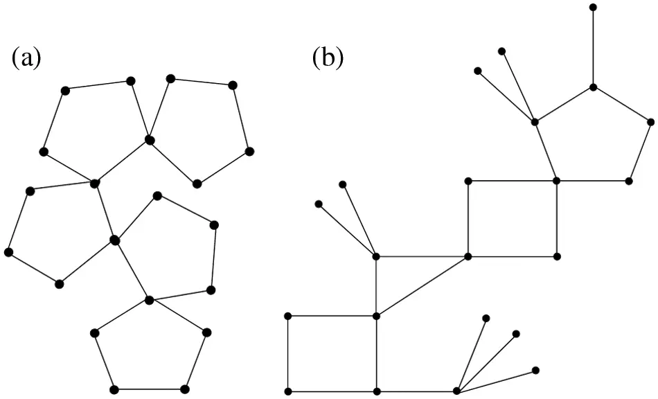
Figure 1: Cactus graphs: (a) is polygonal and (b) is non-polygonal

Let Vj={νij:1≤i≤κ} be the set of vertices in jth κ-cycle of a polygonal cactus for 1≤j≤n. Then the vertex set of the cactus is ∪j=1nVj. The aim of this paper is to explore the metric identification of vertices in polygonal cacti. We investigate the minimum number of vertices which perform the metric identification in chain and star polygonal cacti. It is worth noticing that the metric identification of certain graphs have been studied [19,20]. However, this notion has not been explored for the chain and star polygonal cacti which makes the paper different from the available literature.

2  Chain Polygonal Cactus

A chain polygonal cactus, denoted by Tn,κ, is a class of polygonal cactus in which each polygon has at most two cut vertices, where n is the number of κ-polygons, known as the length of Tn,κ.

Lemma 2.1. For κ≥3 with n≥2, if S is a metric generator for Tn,κ, then S must contain at least one vertex from both the end blocks of Tn,κ.

Proof. Without loss of generality, suppose that S does not contain any vertex from the first block of Tn,κ. Then for two vertices x, y such that x∼ν1 and y∼ν1 (ν1 is the cut vertex between first and second polygons of Tn,κ), we have mS(x)=mS(y), a contradiction.

According to the definition, cactus chain Tn,κ has exactly n−2 non-pendent polygons and two pendent polygons. For n≥3, Tn,3 is unique. However, Tn,κ is not unique for κ≥4 and n≥3. Hereafter, we define two special classes of cactus chains for κ≥4 and n≥3.

2.1 Tn,κ with Adjacent Cut Vertices

In Tn,κ, if we let νκj=ν1j+1=νj (a joint/cut vertex between jth and (j+1)th polygons/cycles) for 1≤j≤n−1, then cut vertices in Tn,κ are adjacent, and this type of chain polygonal cactus is denoted by Hn,κ. In fact, cut-vertices in Hn,κ, lying in the same non-pendent polygon, are adjacent. See Fig. 2.

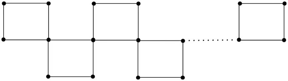
Figure 2: A 4-polygonal chain cactus with adjacent cut vertices

Lemma 2.2. For κ,n>3, it is not possible that two consecutive blocks do not contribute to form a metric generator for Hn,κ.

Proof. Contrarily, suppose that two consecutive blocks Bi and Bi+1 do not contribute to form a metric generator S for Hn,κ. Then, there are BDS x in Bi and y in Bi+1 and both x and y are neighbors of the joint νi, such that no vertex s∈S identified x and y. So, S is not a metric generator for Hn,κ, a contradiction.

Theorem 2.1. For n≥3, dim(Hn,3)=2.

Proof. By Theorem 1.1, only path graph has metric dimension equal to 1, so dim(Hn,3)≥2. Let W={ν11,ν3n} be a set of vertices of Hn,3, then metric vectors of all the vertices in Hn,3 with respect to W are:

mW(ν11)=(0,n−1), mW(ν3n)=(n−1,0),

mW(νj)=(j,n−j) for 1≤j≤n−1,

mW(ν2j+1)=(1+j,n−j) for 0≤j≤n−1.

We can see that all the metric vectors are distinct. So, W is a metric generator for Hn,3, and therefore dim(Hn,3)=2.

Theorem 2.2. For odd κ≥5, dim(H3,κ)=2.

Proof. By Theorem 1.1, only path graph has the metric dimension equals to 1. So, dim(H3,κ)≥2. Further, consider W={νκ−121,νκ+123}, and accordingly metric vectors of the vertices are:

mW(νi1)={(κ−12−i,κ+12+i),1≤i≤κ−32,(i+1−κ2,3κ+12−i),κ−12<i≤κ−1,(κ−12,κ+12),i=κ.

mW(νi2)={(κ−32+i,κ−12+i),1≤i≤κ−12,(i+κ−32,3κ−12−i),i=κ+12,(3κ+12−i,3κ−12−i),κ+12<i≤κ.

mW(νi3)={(κ−12+i,κ+12−i),1≤i≤κ+12,(3κ+32−i,i−κ+12),κ+12<i≤κ.

Obviously for every two vertices x, y of H3,κ with x≠y, mW(x)≠mW(y). Thus, W is a metric generator for H3,κ and dim(H3,κ)≥2.

Lemma 2.3. For even κ≥4, if S is a minimum metric generator for H4,κ, then |S|≥4.

Proof. We contrarily assume that |S|=3. By Lemma 2.1, S must contain one vertex from each end block. Let a vertex u be taken from the block B1 and a vertex w be taken from the block B4. Then S does not contain any vertex from one of the remaining two blocks. Without loss of generality, we suppose that S does not contain any vertex from block B3, then we have two possibilities:

1.    Whenever d(u,ν1)≠κ2≠d(w,ν3), then there are two vertices x and y, both are the neighbors of the joint ν3, such that they are BDS in H4,κ and mS(x)=mS(y), a contradiction.

2.    Whenever d(u,ν1)=κ2 (ord(w,ν3)=κ2), then there are two vertices x and y both are lying in the block B1 (or B3) and the neighbors of the joint ν1(or ν3) such that they are BDS in H4,κ and mS(x)=mS(y), a contradiction.

Hence, our supposition is wrong and |S|≥4.

Theorem 2.3. For even κ≥4, dim(H4,κ)=4.

Proof. Lemma 2.3 provides the lower bound for dim(H4,κ).

Now, we prove that dim(H4,κ)≤4. For this, let S={νκ2+11,νκ2+12,νκ2+13,νκ4}, and we have to show that for any pair (x, y) of vertices in H4,κ, there is always a vertex in S which identifies the pair (x, y). For this, we consider three cases:

Case-I Whenever x, y belong to the same block Bi of H4,κ, then there are two possibilities:

1.    If x and y are BDS, then a vertex in S, chosen from the block Bi, will identifies the pair (x, y).

2.    If x and y are not BDS, then d(x,ν)≠d(y,ν), where ν is the cut vertex of a cycle Ci. Thus, d(x,s)≠d(y,s) for at least one vertex s of S lying in the block Bi+1 (or in the block Bi−1).

Case-II If x, y do not belong to the same block Bi, then there are two possibilities:

1.    When x belongs to the block Bi and y belongs to the block Bi+1 (or Bi−1). If x and y are BDS, then there is a vertex of S lying either in the block Bi or Bi−1 or Bi+1, which identifies the pair (x, y). Otherwise, there is always a vertex s in S lying in the block containing x or y such that d(x,s)≠d(y,s).

2.    If x and y do not belong to the two adjacent blocks, i.e., x∈Bi and y∈Bj for j≠i+1 and i−1, then we always find a vertex w of S lying in Bi (or Bj) such that d(x,w)≠d(w,y).

Case-III Whenever x or y or both x and y is (are) a joint (s), then there are two possibilities:

1.   If x and y are adjacent, then there is a vertex u∈S, such that d(x,u)=1+d(y,u) where u and y lie on a same cycle, or d(y,u)=d(x,u)+1 where u and x lie on a same cycle. Accordingly, u identifies the pair (x, y).

2.   If x and y are not adjacent, then there are s1,s2 in S such that s1,x lie on the same cycle Ci (say) and s2,y lie on the a same cycle Cj, where j≠i,i+1,i−1. In this case, both s1 and s2 identify the pair (x, y), because

d(x,s2)=d(y,x)+d(y,s2) andd(y,s1)=d(x,y)+d(x,s1).

According to all these cases, it can be concluded that S is a metric generator of H4,κ.

Lemma 2.4. For even κ≥4 and any n≥3 with n≠4, if S is a minimum metric generator for Hn,κ, then |S|≥[n2]+2.

Proof. Let [n2]+2=m and S has two vertices x and y (say) from end blocks B1 and Bn respectively, by Lemma 2.1. Next, we show that S must contain at least m−2 more vertices from Hn,κ. Contrarily, assume that S contains m−3 more vertices. There are two claims to discuss:

Claim-1 Whenever d(x,ν1)=κ2 (ord(y,νn−1)=κ2), then S must contain one more vertex from B1 (or Bn).

Neighbors u and ν of x (or y) satisfy mS(u)=mS(ν), so S is not a metric generator. In this way, we get two consecutive blocks among them no vertex will contribute in S, because S contains m−3 more vertices from (n−2) blocks. It yields a contradiction of Lemma 2.2.

Claim-II Whenever d(x,ν1)≠κ2≠d(x,νn−1), then S must have at least one vertex from both the blocks B2 and Bn−1.

We suppose that S does not contain a vertex from the block B2 (say). Then there are two vertices, u1 in the block B1 and w1 in the block B2, such that mS(u1)=mS(w1), where u1∼ν1∼w1. So, S is not a metric generator. Thus our claim is true. Now, S must have at least one vertex from both the block B2 and Bn−1, and S must contain m−3 vertices from (n−2) blocks. So, there always exist two consecutive blocks from each and among them no vertex will contribute to form the set S, which is contradiction of Lemma 2.2.

Both the claims provide that our assumption is wrong. Hence S must contain at least m−2 more vertices other than x and y, which implies that |S|≥m.

Theorem 2.4. For even κ≥4 and any n≥3 with n≠4, dim(Hn,κ)=[n2]+2.

Proof. An establishment of upper and lower bounds for dim(Hn,κ) will complete the proof.

Lower bound: Lemma 2.4 provides the minimum metric generator for Hn,κ of cardinality [n2]+2, which yields the lower bound.

Upper bound: We discuss two cases according to the parity of n.

•   When n≥6 is even. Let W={νκ2+11,νκ2+12,νκ2+12i+1,νκn;1≤i≤n−22}. Then, with the similar reasoning given in the proof of Theorem 2.3 for the upper bound, the set W is a metric generator for Hn,κ.

•   When n≥3 is odd. Let S={νκ2+11,νκ22i,νκn;1≤i≤n−12}. Let p=(νtr,νum) be any arbitrary pair of vertices in Hn,κ. To prove that S is a metric generator, we have to show that there always a vertex in S which identifies the pair p. We will discuss three possibilities:

Possibility 1: When r=m, then we always have a vertex s∈S such that s∈Br+1 or s∈Br−1 and s identifies the pair p.

Possibility 2: When r∈{m,m+1,m−1}, then there is a vertex s in S from the block Br (or Bm) such that s identifies the pair p.

Possibility 3: When r∉{m−1,m,m+1}, then at least one of the following two observations must true:

•   S contains an element s from the block Br (or Bm) such that s identifies the pair p.

•   S contains an element s from the block Br+1 (or Bm+1) such that s identifies the pair p.

Hence, S is a metric generator for Hn,κ.

Lemma 2.5. For odd κ≥5 and any n≥4, if S is a minimum metric generator for Hn,κ, then |S|≥[n2]+1.

Proof. Let [n2]+1=l. By Lemma 2.1, S must have two vertices from both the end blocks of Hn,κ. Now, we have to show that S contains at least l−2 more vertices. Contrarily, assume that S contains l−3 more vertices. Then, with the similar reasoning given in the proof of Lemma 2.4, we get two consecutive blocks such that none of them contributes in the set S, which is a contradiction of Lemma 2.2. So, our supposition is wrong. Hence, S must contain at least l−2 more vertices, which implies that |S|≥l.

Theorem 2.5. For odd κ≥5 and any n≥4, dim(Hn,κ)=[n2]+1.

Proof. dim(H4,κ)≥[n2]+1, by Lemma 2.5. Moreover, with the similar justification proposed for the proof of upper bound in Theorem 2.4, Hn,κ has a metric generator W={νκ2+12i−1,νκn;1≤i≤n2} when n is even, and has a metric generator W={νκ22i−1;1≤i≤n+12} when n is odd. It follows that dim(Hn,κ)≤[n2]+1.

2.2 Tn,κ with Non Adjacent Cut Vertices

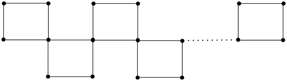
Rn,κ denotes a chain cactus Tn,κ such that the cut-vertices, lying in the same non-pendent polygon of Tn,κ, are not adjacent, see Fig. 3. We further classify Rn,κ into three types:

•   Whenever κ is even and the distance between cut vertices is κ2, then we let νκ2+1j=ν1j+1=νj (a joint/cut vertex between jth and (j+1)th polygons/cycles) for 1≤j≤n−1.

•   Whenever κ is odd and the distance between cut vertices is κ−12, then we let νκ+12j=ν1j+1=νj (a joint/cut vertex between jth and (j+1)th polygons/cycles) for 1≤j≤n−1.

•   Without loss of generality, we let νκ−1j=ν1j+1=νj, otherwise (a joint/cut vertex between jth and (j+1)th polygons/cycles) for 1≤j≤n−1.

Figure 3: A 5-polygonal chain cactus with non-adjacent cut vertices

With the similar justification proposed for the proof of Lemma 2.2, we have the following result:

Lemma 2.6. For κ>5 and n≥3, it is not possible that two consecutive blocks do not contribute to form any metric generator for Rn,κ.

Theorem 2.6. For odd κ≥3, dim(R2,κ)=2.

Proof. Since only a path graph has the metric dimension equals to 1, by Theorem 1.1, dim(R2,κ)≥2. Now, we have to prove that dim(R2,κ)≤2 by investigating a metric generator of cardinality 2. Let us consider the set of vertices W={ν11,νκ+122}. Then, metric vectors of all the vertices in R2,κ with respect to W are:

mW(νi1)={(i−1,i+κ−12),1≤i<κ−12,(κ−32,κ−1),i=κ−12,(k−i+1,3κ−12−i),κ−12<i≤κ.

mW(νi2)={(i,κ+12−i),1≤i≤κ+12,(κ−i+2,i−κ+12),κ+12<i≤κ.

It can be easily verified that for every pair x, y of distinct vertices, we have mW(x)≠mW(y). So, W is a metric generator for R2,κ, and dim(R2,κ)≤2.

Theorem 2.7. For even κ≥4, dim(R2,κ)=3.

Proof. The proof follows from the following two claims:

Claim I: (dim(R2,κ)≥3)

Suppose contrarily that dim(R2,κ)<3. Since any metric generator for R2,κ must contain a vertex from both end blocks, by Lemma 2.1, dim(R2,κ)≥2. Let S={x,y} be a minimum metric generator for R2,κ, where x∈B1 and y∈B2. Then, there are two possibilities:

1.    Whenever d(x,νκ1)=κ2 or d(y,ν12)=κ2, then there are two vertices u1 and u2, lying in the same block and both are neighbors of the joint, such that ms(u1)=ms(u2), a contradiction.

2.    Whenever d(x,νκ1)≠κ2≠d(y,ν12), then there are two vertices w1 (lying in the block B1), and w2 (lying in the block B2) such that w1, w2 are neighbors of the joint and ms(w1)=ms(w2), a contradiction.

Thus, according to these possibilities, S is not a metric generator. So, our supposition is wrong and dim(R2,κ)≥3.

Claim II: (dim(R2,κ)≤3)

Let us consider a set S={ν11,ν22,νκ−22} of vertices. Then, metric vectors of the vertices of R2,κ with respect to S are:

mS(νi1)={(i−1,1+i,i+1),1≤i≤κ2−2,(κ2−2,κ2,κ2−1),i=κ2−1,(κ2−1,κ2+1,κ2−2),i=κ2,(κ2,κ2,κ2−2),i=κ2+1,(κ−i+1,κ−i+1,κ−i+2),κ2+1<i≤κ−2,(2,2,1),i=κ−1,(1,1,2),i=κ.

mS(νi2)={(1,1,2),i=1,(κ−i+2,i−2,1+i),2≤i≤κ2+1,(κ2+2,κ2,κ2+3),i=κ2+2,(κ2+2,κ−i+2,κ−i+1),κ2+2<i≤κ.

It can be seen that all the metric vectors are different, which implies that S is a metric generator for R2,κ. Hence dim(R2,κ)≥3.

Let u,ν∈V(G) be any two vertices. Then, u,ν are called twins if either N[u]=N[ν] or N(u)=N(ν). The relation of twins between vertices of G is an equivalence relation, which partitioned V(G) into classes each of which is called a twin class. A twin class may be singleton [6]. The following results are useful tools to identify twins in a graph G.

Lemma 2.7. [6] If u and ν are twins in a connected graph G, then no vertex, except u and ν, of G identifies the vertices u and ν.

Accordingly, we have the following remark:

Remark 2.1. If U is twin class in a connected graph G with |U|=l≥2, then every metric generator for G contains at least l−1 vertices from U.

Theorem 2.8. For n≥3, dim(Rn,4)=n.

Proof. We prove the result with two cases providing lower and upper bounds for the metric dimension of Rn,4.

Case-I (Lower bound)

In Rn,4, we obtain n twin classes each of them has cardinality 2. Now, if S is a minimum metric generator for Rn,4, then S must contain at least one vertex from each twin class, by Remark 2.1. This implies that dim(Rn,4)=|S|≥n.

Case-II (Upper bound)

Let S={ν31,ν2t:2≤t≤n}⊂V(Rn,4). Then, S is a metric generator for Rn,4, because all the vertices have distinct metric vectors with respect to S as listed below:

for fixed 1≤j≤n,

mS(ν11)=(a1j,a2j,…,anj), where the lth coordinate is

alj={2l−1,for1≤l≤n.

mS(ν2j)=(a1j,a2j,…,anj), where the lth coordinate is

alj={2(j−l),whenever1≤l<j,0,wheneverl=j,2(l−j),wheneverj<l≤n.

mS(ν3j)=mS(ν1j+1)=(a1j,a2j,…,anj), where the lth coordinate is

alj={2j−2l+1,whenever1≤l<j,1,wheneverl=j,2l−2j−1,wheneverj<l≤n.

mS(ν4j)=(a1j,a2j,…,anj), where the lth coordinate is

alj={2(j−l),whenever1≤l<j,2,wheneverl=j,2(l−2j),wheneverj<l≤n.

This implies that dim(Rn,4)≤n.

Lemma 2.8. For even κ≥6, if S is a minimum metric generator for R3,κ, then |S|≥3.

Proof. By Lemma 2.1, S must contain a vertex from both the end blocks of R3,κ. Suppose that a 2-element set S={x,y} is a metric generator for R3,κ, where x lies in the block B1 and y lies in the block B3. We will discuss two possibilities:

1.    Whenever d(x,ν1)=κ2, then there are vertices u1, w1 in the block B1 such that u1 and w1 are BDS and u1∼ν1∼w1. It follows that mS(u1)=mS(w1), a contradiction to the fact that S is a metric generator. Similarly, if d(y,ν2)=κ2, then again we get a contradiction.

2.    Whenever d(x,ν1)≠κ2≠d(y,ν2), then there are two vertices, u2 in B1 and w2 in B2, such that u2∼ν1∼w2 and

    Hence mS(u2)=mS(w2), a contradiction. Similarly, there are two vertices u3, w3 both are the neighbors of the joint ν2, such that mS(u3)=mS(w3), a contradiction.

d(u2,x)=1+d(ν1,x),d(w2,x)=1+d(ν1,x).

It follows that our supposition is wrong, and no 2-element set is a metric generator for R3,κ. Thus |S|≥3.

Theorem 2.9. For even κ≥6, dim(R3,κ)=3.

Proof. By Lemma 2.8, dim(R3,κ)≥3. Moreover, dim(R3,κ)≤3, because the set S={νκ1,ν23,ν22} is a metric generator for R3,κ due to the following distinct metric vectors of the vertices with respect to S:

mS(νl1)={(l,l+4,l+2),1≤l≤κ2−1,(κ−l,κ−l+2,κ−l),κ2−1<l≤κ−1,(0,4,2),l=κ.

mS(νl2)={(1,3,1),l=1,(l,l+2,l−2),2≤l≤κ2−1,(l,κ−l,l−2),κ2−1<l≤κ2+2,(l,κ−l,κ−l+2),κ2+2<l≤κ−2,(κ−l+2,κ−l,κ−l+2),l=κ−1,(κ−l+2,2,κ−l+2),l=κ.

mS(νl3)={(3,1,3),l=1,(l+2,l−2,l+2),2≤l≤κ2+1,(κ−l+4,κ−l+2,κ−l+4),κ2+1≤l≤κ.

Theorem 2.10. For even κ≥6, dim(R4,κ)=4.

Proof. Let S={ν11,ν22,ν23,ν24}⊂V(R4,κ). Then the metric vector of νlj with respect to S is given below:

mS(νl1)={(l−1,l+2,l+4,l+6),1≤l≤κ2−1,(κ−l+1,κ−l+2,κ−l+4),κ2−1<l≤κ−1,(1,2,4,6),l=κ.

mS(νl2)={(2,1,3,5),l=1,(l+1,l−2,l+2,l+4),2≤l≤κ2−1,(κ2+1,κ2+1−2,κ2,κ2+1+2),l=κ2,(κ−l+3,κ−l+2,κ−l,κ−l+2),κ2+1≤l≤κ−1,(3,2,2,4),l=κ.

mS(νl3)={(4,3,1,3),l=1,(l+3,l+2,l−3,l+2),2≤l≤κ2−1,(κ2+3,κ2+2,κ2−2),l=κ2,(κ−l+5,κ−l+4,κ−l+2,κ−l),κ2+1≤l≤κ−1,(5,4,2,2),l=κ.

mS(νl4)={(6,5,3,1),l=1,(5+l,4+l,2+l,2−l),2≤lκ2+1,(κ−l+7,κ−l+6,κ−l+4,κ−l+2),κ2+1≤l≤κ.

It can easily verify that all metric vectors are distinct. Thus, S is a metric generator for R4,κ and dim(R4,κ)≤4.

Now, we claim that if S is a minimum metric generator for R4,κ, then |S|≥4. Suppose contrarily that |S|=3. By Lemma 2.1, S must contain one vertex from both the end blocks of R4,κ. Let S={x,y,z}, where x lies in the first block B1 and y lies in the last block B4. There are two cases to discuss:

1.    If z lies in the block B1 (or B4), then there exist BDS, u1 lies in the block B2 and w1 lies in the block B3 with u1∼ν2∼w1, such that mS(u1)=mS(w1), a contradiction.

2.    If z lies in the block B2 (or B3) and, without loss of generality, we suppose that z lies in the block B2, then there are two possibilities:

•      Whenever d(x,ν1)=κ2 (ord(y,ν3)=κ2), then there are BDS, u2 and w2 lying in the block B1(or in the block B4), such that both are the neighbors of joint ν1 (or ν3) and mS(u2)=mS(w2), a contradiction to the fact that S is metric generator.

•      Whenever d(x,ν1)≠κ2≠d(y,ν3), then there are BDS, u3 lies in the block B3 and w3 lies in the block B4 such that u3∼ν3∼u3 and mS(u3)=mS(ν3), we get a contradiction.

All these possibilities conclude that our supposition is wrong and |S|≥4. Hence, dim(R4,κ)≥4.

Theorem 2.11. For n≥3, dim(Rn,5)=2.

Proof. By Theorem 1.1, only a path graph has the metric dimension equals to 1. Therefore, dim(Rn,5)≥2. Now, consider a set W={ν11,ν3n} of vertices of Rn,5. Then, metric vectors of the vertices with respect to W are:

mW(νl1)={(1−l,3−l+2(n−1)),l=1,(l−1,3−l+2(n−1)),1<l≤3,(6−l,l+2n−5),3<l≤5.

For 2≤j≤n,

mW(νlj)={(l+2(j−2),3−l+2(n−j)),1≤l≤3,(3−l+2j,2(n−j)+l−3),3<l≤5.

It can easily verify that for each pair of distinct vertices (x, y) in R3,κ, we have mW(x)≠mW(y). Thus, W is a metric generator for Rn,5 and dim(Rn,5)≤2. It completes the proof.

According to the similar reasoning of the proofs of Theorems 2.4 and 2.5 we have the following two results for Rn,κ.

Theorem 2.12. For even κ≥6 and any n≥5, dim(Rn,κ)=[n2]+2.

Theorem 2.13. For odd κ≥7 and any n≥3, dim(Rn,κ)=[n2]+1.

Theorem 2.14. For even κ≥6 and any n≥3, whenever d(νi,νi+1)=κ2 in Rn,κ for each 1≤i≤n−1, then dim(Rn,κ)=n.

Proof. Let S be a minimum metric generator and assume that |S|=n−1. This implies that S does not have any vertex from at least one block Bt (say), then we have two vertices u,w∈Bt such that u and w are BDS, u∼νt−1 (orνt), w∼νt−1 (orνt) and mS(u)=mS(w). This is a contradiction to the fact that S is a metric generator for Rn,κ. Hence dim(Rn,κ)=|S|≥n.

Now, let S={νκ2−1i:1≤i≤n}⊂V(Rn,κ). Then, with the similar reasoning as given for the proof of upper bound in Theorem 2.3, S is a metric generator for Rn,κ. It follows that dim(Rn,κ)≤n.

Theorem 2.15. For odd κ≥7 and any n≥3, whenever d(νi,νi+1)=κ−12 in Rn,κ for each 1≤i≤n−1, then dim(Rn,κ)=2.

Proof. By Theorem 1.1, dim(Rn,κ)≥2, because Rn,κ is not a path graph. Now, let W={νκ−321,νκ+12n} and corresponding metric vectors of the vertices are:

mW(νi1)={(κ−52−i+1,κ+12−i+κ−12(n−1)−κ−12(j−1)),1≤i≤κ−32,(i−κ−32,κ+12−i+κ−12(n−1)−κ−12(j−1)),κ−32<i≤κ+12,(i−κ−32,κ−32+i+κ−12(n−3)−κ−12(j−1)),κ+12<i≤κ−2,(3κ−32−i,κ−32+i+κ−12(n−3)−κ−12(j−1)),κ−2<i≤κ.

For 2≤j≤n,

mW(νij)={(i+κ−32+κ−12(j−2)−1),κ+12−i+κ−12(n−1)−κ−12(j−1)),1≤i≤κ+12,(3κ−12−i+κ−12(j−2)),κ−32+i+κ−12(n−3)−κ−12(j−1)),κ+12<i≤κ.

It can easily verify that for every two distinct vertices x, y of Rn,κ, we have mW(x)≠mW(y). It follows that W is a metric generator for Rn,κ and dim(Rn,κ)≥2. It concludes the proof.

2.3 Star Polygonal Cactus

A star polygonal cactus is a κ-polygonal cactus in which all polygons have a common cut vertex. It is denoted by Wn,κ, where n represents number of polygons Cκ. A star polygonal cactus contains exactly one vertex of degree 2n and all other vertices have degree two that is why Wn,κ is considered to be a unique and special type of cactus graph. Mathematically, if νκ1=νκ2=…=νκn=J (a cut-vertex/joint), then V(Wn,κ)={J}∪j=1n(V(Cκ)−{νκj}) and E(Wn,κ)=∪j=1nE(Cκ).

References

1. Khuller, S., Raghavachari, B., Rosenfeld, A. (1996). Landmarks in graphs. Discrete Applied Mathematics, 70(3), 217–229. DOI 10.1016/0166-218X(95)00106-2. [Google Scholar] [CrossRef]
2. Melter, F., Harary, F. (1976). On the metric dimension of a graph. Ars Combinatoria, 2, 191–195. [Google Scholar]
3. Slater, P. J. (1975). Leaves of trees. Proceedings of the sixth Southeastern Conference on Combinatorics, Graph Theory, and Computing, Florida Atlantic University, vol. 14, pp. 549–559. Boca Raton. [Google Scholar]
4. Chartrand, G., Eroh, L., Johnson, M. A., Oellermann, O. R. (2000). Resolvability in graphs and the metric dimension of a graph. Discrete Applied Mathematics, 105(1–3), 99–113. DOI 10.1016/S0166-218X(00)00198-0. [Google Scholar] [CrossRef]
5. Salman, M., Javaid, I., Chaudhry, M. A. (2012). Resolvability in circulant graphs. Acta Mathematica Sinica, English Series, 28(9), 1851–1864. DOI 10.1007/s10114-012-0417-4. [Google Scholar] [CrossRef]
6. Khalid, I., Ali, F., Salman, M. (2019). On the metric index of circulant networks–An algorithmic approach. IEEE Access, 7, 58595–58601. DOI 10.1109/ACCESS.2019.2914933. [Google Scholar] [CrossRef]
7. Ahmad, S., Chaudhry, M. A., Javaid, I., Salman, M. (2013). On the metric dimension of generalized petersen graphs. Quaestiones Mathematicae, 36(3), 421–435. DOI 10.2989/16073606.2013.779957. [Google Scholar] [CrossRef]
8. Imran Javaid, S. A., Azhar, M. N. (2012). On the metric dimension of generalized petersen graphs. Ars Combinatoria, 105, 171–182. [Google Scholar]
9. Naz, S., Salman, M., Ali, U., Javaid, I., Bokhary, S. A. U. H. (2014). On the constant metric dimension of generalized petersen graphs p (n, 4). Acta Mathematica Sinica, English Series, 30(7), 1145–1160. DOI 10.1007/s10114-014-2372-8. [Google Scholar] [CrossRef]
10. Alsaadi, F. E., Salman, M., Ali, F., Khalid, I., Cao, J. et al. (2020). An algorithmic approach to compute the metric index of chordal ring networks. IEEE Access, 8, 80427–80436. DOI 10.1109/ACCESS.2020.2990913. [Google Scholar] [CrossRef]
11. Manuel, P. D., Rajasingh, I. (2011). Minimum metric dimension of silicate networks. Ars Combinatoria, 98, 501–510. [Google Scholar]
12. Manuel, P., Rajan, B., Rajasingh, I., Monica, M. C. (2006). Landmarks in torus networks. Journal of Discrete Mathematical Sciences and Cryptography, 9(2), 263–271. DOI 10.1080/09720529.2006.10698077. [Google Scholar] [CrossRef]
13. Rajan, B., Sonia, K., Chris Monica, M. (2011). Conditional resolvability of honeycomb and hexagonal networks. Mathematics in Computer Science, 5(1), 89–99. DOI 10.1007/s11786-011-0076-3. [Google Scholar] [CrossRef]
14. Jannesari, M., Omoomi, B. (2012). The metric dimension of the lexicographic product of graphs. Discrete Mathematics, 312(22), 3349–3356. DOI 10.1016/j.disc.2012.07.025. [Google Scholar] [CrossRef]
15. Cáceres, J., Hernando, C., Mora, M., Pelayo, I. M., Puertas, M. L. et al. (2007). On the metric dimension of cartesian products of graphs. SIAM Journal on Discrete Mathematics, 21(2), 423–441. DOI 10.1137/050641867. [Google Scholar] [CrossRef]
16. Peters-Fransen, J., Oellermannt, O. (2006). The metric dimension of cartesian products of graphs. Utilitas Mathematica, 69, 33–41. [Google Scholar]
17. Yero, I. G., Kuziak, D., Rodríguez-Velázquez, J. A. (2011). On the metric dimension of corona product graphs. Computers & Mathematics with Applications, 61(9), 2793–2798. DOI 10.1016/j.camwa.2011.03.046. [Google Scholar] [CrossRef]
18. Ye, J., Liu, M., Yao, Y., Das, K. C. (2019). Extremal polygonal cacti for bond incident degree indices. Discrete Applied Mathematics, 257, 289–298. DOI 10.1016/j.dam.2018.10.035. [Google Scholar] [CrossRef]
19. Khali, A., Husain, S. K. S., Faisal, N. M. (2022). On bounded partition dimension of different families of convex polytopes with pendant edges. AIMS Mathematics, 7(3), 4405–4415. DOI 10.3934/math.2022245. [Google Scholar] [CrossRef]
20. Nadeem, M. F., Qu, S., Ahmad, A., Azeem, M. (2022). Metric dimension of some generalized families of toeplitz graphs. Mathematical Problems in Engineering, 2022, 9155291. DOI 10.1155/2022/9155291. [Google Scholar] [CrossRef]
21. Javaid, I., Rahim, M. T., Ali, K. (2008). Families of regular graphs with constant metric dimension. Utilitas Mathematica, 75(1), 21–33. [Google Scholar]
Submit a Paper
Propose a Special lssue
Open Access
View Full Text
Download PDF
Copyright © 2023 The Author(s). Published by Tech Science Press.
Downloads
Citation Tools