Health Monitoring of Milling Tool Inserts Using CNN Architectures Trained by Vibration Spectrograms

1  Introduction

In subtractive machining processes, the desired surface finish of a job is achieved by the controlled removal of material [1]. Conventional methods such as turning, milling, and drilling are principally practiced processes in the industry [2]. Most of the research attention has been directed towards the milling process owing to its versatile and wide-ranging applications [3]. Milling is an intermittent cutting operation performed using a controlled cutting tool configured with multiple inserts [4]. Thus, in-process damage to a cutting tool degrades the surface finish of the job shaped by machining and causes a significant financial loss [5]. Therefore, the subject of tool condition monitoring is being persuaded through various approaches, such as diagnostic, prescriptive, predictive, as well as descriptive ones, and has emerged as a field worth investing in view of Industry 4.0 [6]. The predictive approach forecasts the possible failure of a cutting tool based on historic data and is helpful in preventive maintenance [7]. Most of the study is inclined toward the prediction of tool wear through the design of deep networks [8]. The diagnostic and prescriptive approach has been practiced for decades in an offline mode and is referred to as root cause analysis [9,10]. The diagnostic approach clarifies the reason behind the problem and the prescriptive approach suggests that action needs to be taken to solve the problem [11,12]. The descriptive approach characterizes the problem and the predictive approach helps in its prevention [13,14]. Researchers have adapted a descriptive approach through ML models capable of characterizing the cutting tool condition [15,16]. Li et al. [17] presented a comprehensive review based on structures of aero-engine rotors for analyzing their reliability. The surrogate models are recommended owing to their strong computational efficiency in terms of time and development procedure. Cherid et al. [18] presented optimization of the number of sensors and their placement in order to detect and localize the failure in bridge structure through the integration of Principle Component Analysis and Artificial Neural Net reduced FRF technique. Luo et al. [19] presented structural reliability analysis using the ML approach and hybrid novel Monte Carlo simulations for turbine bladed disk and laminated composite plate. This model showcases the greater flexibility in the prediction of failure over enhanced Monte Carlo simulation and it is efficient computationally with high-nonlinear problems. In an era of intelligent data analytics, the predictive approach has been reformed in an intelligent way by designing various ML and DL models capable of predicting the remaining useful life of a cutting tool [20].

Most of the similar models being trained on exact and limited instances lack key features of generalization when deployed in a high noise environment of cross-domain machining and versatile process parameters. In order to provide descriptive analytics for similar situations, a deep learning framework is achieving substantial consideration and can be configured in desired ways. Once the approach is established, this can be further extended to diagnostic and prescriptive approaches in a similar manner. In the case of vibration signal processing, STFT is used for processing and analyzing signals of non-stationary nature by splitting them as segments of narrow time periods and taking each segment’s Fourier transform. As STFT has smaller time windows, subsequently, the spectrum of frequencies varies smoother over time series, therefore it appears more detailed. On the other hand, the model trained on directly sampled numeric vibration data may not yield real results. Thus, the STFT spectrogram breaks the time-domain response of vibration into the chain of folds and takes the Fast Fourier transform of all folds. This chain of FFT folds is then overlapped for visualizing how the magnitude and frequencies of the changes over a change in time. This transformation makes the 3D surface plot of FFTs and includes a scale of different colors and shades for representing and constructing a spectrogram image. A very first and important reason is that the deep learning algorithms work very efficiently on image-based datasets as they can be processed in multiple dimensions as compared to numeric datasets. Also, the information gained from images can be integrated into the time-series signals and has useful to make generalized robust models with fast convergence. Thus, classification using image-based datasets is advocated herein instead of using raw vibration signals in numeric form. Deep learning, a primary subclass of machine learning, has well established well for processing numeric as well as image-based data through the formulation of “Deep” structure, hierarchical compositionality, distributed representation, and end-to-end learning of Neural Nets. With this motivation, the design of different CNN (Convolutional Neural Network) architectures such as AlexNet, ResNet-50, LeNet-5, and VGG-16 is presented in this paper. Real-time spindle vibrations corresponding to healthy and various faulty configurations of milling cutter were acquired. This data was transformed into the time-frequency domain and further processed by proposed architectures in graphical form, i.e., spectrogram. The model is trained, tested, and validated considering different datasets. The outline of the design, modeling, training and evaluation of CNN architecture algorithms is presented in Fig. 1.

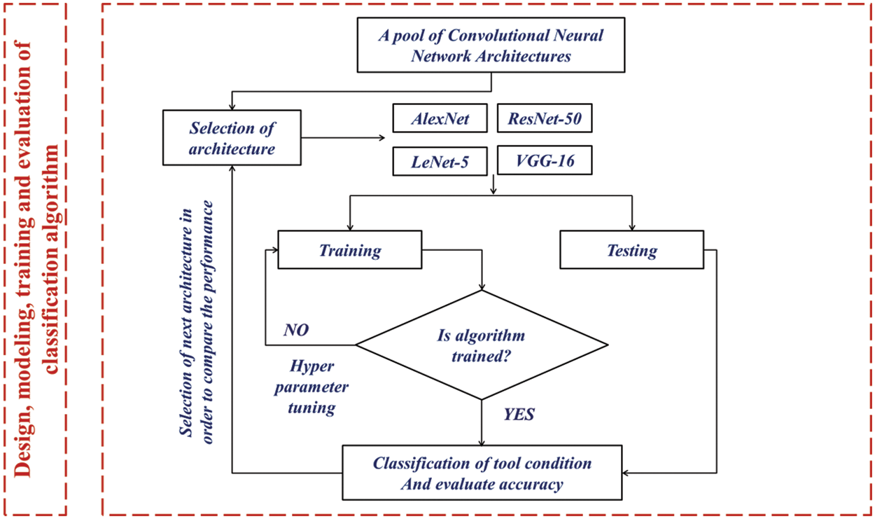
Figure 1: Design, modeling, training and evaluation of classification algorithm

2  Experimental Setup & Data Collection

The experimental study is carried out in an industry named ‘Axis Metal-cut Technologies’ based in Pune, India. The experimental arrangement is represented in Fig. 2. It is comprised of a Vertical Machine Center, a piezoelectric accelerometer (Make: PCB, Model: 352C03 Piezotronics of +/−500 g range & 10 mV/g sensitivity), and a data acquisition card (Vibration analyzer, Model: DEWE 43A with eight channels). The MS workpiece cuboid of 0.65 m × 0.25 m × 0.1 m was positioned using a fixture, and a milling cutter was held securely in the spindle. The milling cutter (diameter 63 mm) consisted of four carbide-coated inserts. With the intention to identify and study the fault classification, the standard machining parameters (cut depth, speed, and table feed) were chosen referring to the standard Komet catalog [21] and mathematical expressions. The speed at which the cutting is achieved was 180 m/min. The feed of the table was approximately 2000 mm/min. Finally, the depth of cut was preferred to be 0.25 mm as per the standard catalog ‘Kom–Guide 2016’ [21]. By considering these machining inputs and tool configuration, face milling operations were performed for 8 configurations, and change in vibration was collected. The 1st tool configuration labeled ‘HADF’ (Healthy tool) was formed using defect-free, i.e., normal inserts. The 2nd to 7th tool configurations labeled ‘FFL, FNS, FNT, FCT, FTB, FBE’ (faulty tool) were formed using defective inserts with flank wear, nose wear, notch wear, crater wear, tip breakage, built-up edge respectively introduced at one position of 4 positions of the tool inserts. The last configuration labeled ‘FAD’ (faulty tool) was formed using all defective inserts (flank wear, nose wear, notch wear, crater wear) introduced at one all 4 positions.

The vibration signals were acquired from the accelerometer considering the setting of sampling length, frequency, and the number of samples to be collected. A moderate sampling length of 8000 was considered. The frequency set for the sampling of vibration signal was 20 kHz according to Nyquist criteria. The Nyquist criteria state that the sampling frequency should be at least twice or more than the top frequency of the raw vibration signal. In this study, considering samples ranging from 50–100, the training data was created for each tool configuration such that it contains at least 2–3 lakh data points. Here 100 samples were considered for each configuration (class) of the milling cutter, and corresponding acceleration signals were collected using the DAQ framework and saved in the comma-delimited data files. This forms training data set of a total of 800 samples. The disturbance caused by vibration produced by environmental conditions is filtered using the suitable low pass and high pass filters which were employed in the data acquisition process. In addition to this, the discrete wavelet transform can also be used to de-noise and decompose the original signal through different mother-child wavelet combinations. Once the data files are collected, signals can be read through graphical illustrations; thus accordingly their representation is essential and described in the next section.

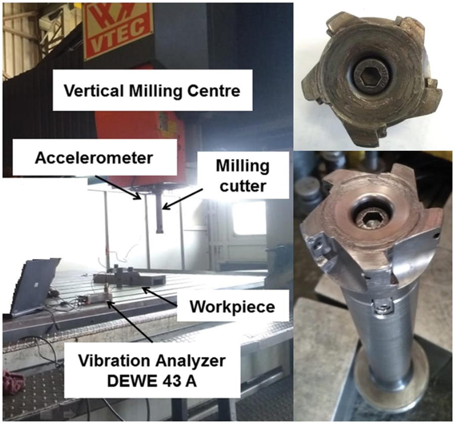
Figure 2: Experimental setup

3  Experimental Setup & Data Collection

The experimentation considering various configurations of milling tools has been performed to collect the data. It is indeed a challenging task to deal with raw data collected through dynamic experimentation. This necessitates the processing of signal that executes its synthesis, modification, and analysis. Signal processing mainly emphasizes detecting components of interest. Initially, the signal is read through graphical illustrations from different orientations. To commence with, the signal is represented in the time-domain and later adapted to spectrogram through the STFT, i.e., Short-time Fourier Transform. The Fourier transform of aperiodic signals is actually the counterpart of the Fourier coefficients in periodic signals [22]. The Discrete Fourier Transform (DFT) is a transform; it describes a relationship between a time sequence and a description of that sequence as a weighted sum of sampled data cosine and sine. The terms FFT and DFT are sometimes used interchangeably. But the DFT is the only one of the four that can be applied to digital data since it consists of a finite number of discrete samples [23]. The Discrete Time Fourier Transform (DTFT) is the dual of the Fourier series, an integral projection from continuous periodic frequency to sampled data time as opposed to an integral projection from continuous periodic time to the sampled data frequency. The DFT is a sample of the Discrete-Time Fourier Transform (DTFT). A transform is a change of variables we start with a variable usually ‘t’ for time and we change to a new variable usually omega for frequency. A series is not a change of variable it’s a different way to write the same function but the variable stays the same. The variable is still ‘t’ though despite the fact that the coefficients of the series are related to the function’s spectrum [24]. A spectrogram is a graphical illustration of the variation of frequency with respect to time or simply depicts the strength of the vibration at a specific time instant. Owing to its graphical illustration, it appears in different colors and shades which is nothing but the measure of the strength of a signal. The bright shade indicates a signal with a higher strength which means the brightness of the shade has direct proportion with the strength of the signal. To summarize, a spectrogram is a fundamentally 2D graph, with a third dimension signified through colors [25–27]. The time-frequency representation of vibration signal depicting different tool configurations is shown in Fig. 3. The image data set consisted of 100 images of each of the 8 tool conditions which gave 800 images.

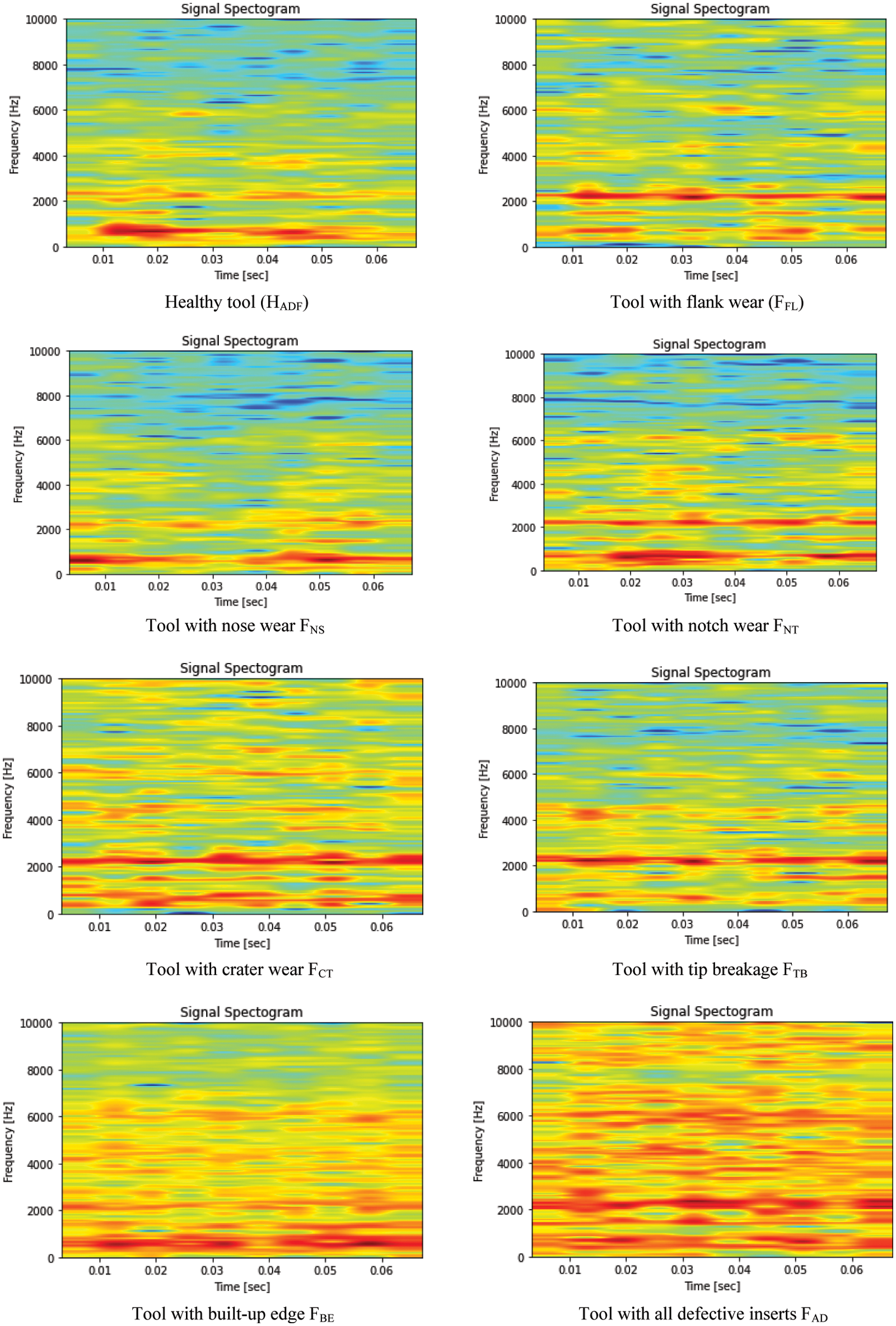
Figure 3: Time-frequency representation of vibration signal depicting different tool configurations

4  Mechanism of CNN Architectures

CNNs are dedicated neural nets explicitly designed for capturing spatial (localized) facts within a data distribution. Through explicitly encoding them in architecture, CNNs are employed to train 2D images or 3D or even 1D data most of the time. The mechanism of CNN architectures (AlexNet, ResNet-50, LeNet-5, and VGG-16) is presented in this section.

4.1 Lenet-5

LeCun et al. [28] designed a pre-trained CNN model in 1998 which was introduced as Lenet-5 for document recognition considering Gradient-Based Learning. The architecture was specially designed for the recognition of printed and handwritten characters. The straightforward and simple architecture of this model was the key feature. The significance of ‘5’ in Lenet-5 is that it has 5 layers with three convolution layers (CL) with averaging pools trailed by double fully connected layers (FCL) as shown in Fig. 4. In the end, the Softmax classifier is connected that performs the classification [29]. The weighted sum (Aj) in classical neural nets aimed at the unit j is handed by the function ‘sigmoid squashing’ for producing the condition of the unit j which is designated by Xj

Xj=f(Aj)(1)

The function ‘sigmoid squashing’ is formulated as follows which is originally a scaled-up hyperbolic tangent:

f(A)=MTanh(SA)(2)

Lastly, the output layer consists of Euclidean-RBF (Radial Basis Function), one for every label, having multiple input features. Output Yj is formulated as

Yi=∑i(Xi−ωji)2(3)

The criteria for sampling training samplers are as follows:

E(W)=1P∑P=1PYDp(Zp,W)(4)

Here, YDp is output and resembles the correct classification of input features Zp.

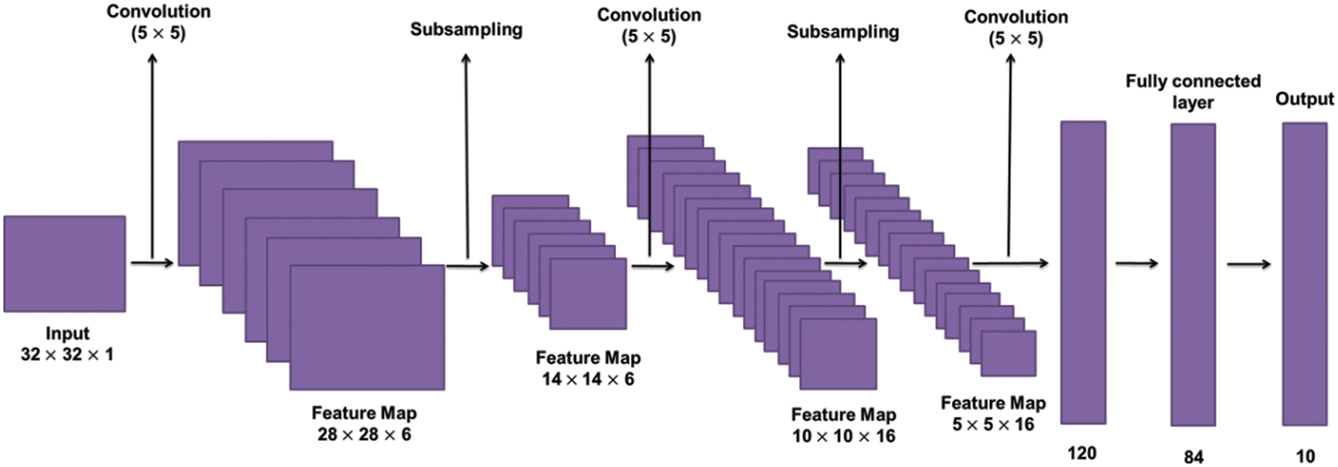
Figure 4: Basic architecture of Lenet [30]

4.2 AlexNet

At first, AlexNet is a significantly popular image classification algorithm that performs well on ImageNet. It’s one of the breakthrough algorithms in computer vision. It is not widely used nowadays, it’s been outperformed by other algorithms that are either less computationally intensive or have better performance on ImageNet [31]. But still, a very interesting architecture to learn! Some of the significant points on AlexNet are discussed here. The AlexNet was split into two networks while training and trained in two GPUs, since it was too large for a single GPU to handle the network [32].

It uses the ReLU activation function in place of the standard tanh function. Since AlexNet had 60 million parameters where ‘Dropout’ and ‘Data augmentation’ techniques were used to take care of the over fitting problem [33]. The standard AlexNet architecture is shown in Fig. 5. The neuron’s output is modeled by considering f designates the function of the input feature x as f(x)=tanh(x) or f(x)=(1+e−x)−1. In the relationship of training time with respect to gradient descent, saturating nonlinearities is very slower than the non-saturating nonlinearity f(x)=max(0,x). The neurons with this nonlinearity as Rectified Linear Units (ReLUs) are preferred. Deep CNNs with ReLUs train much quicker than those of their counterparts with tanh. For case of the CIFAR-10 dataset, iterations desired to attain a training error of 0.25 using the 4-layered convolutional networks. This shows that large neural networks are essential to process such data.

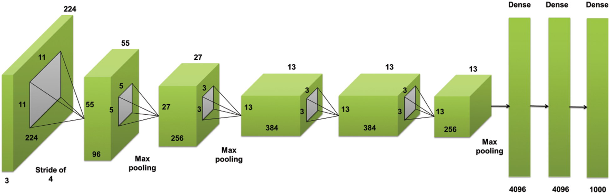
Figure 5: Basic architecture of AlexNet [34]

4.3 ResNet-50

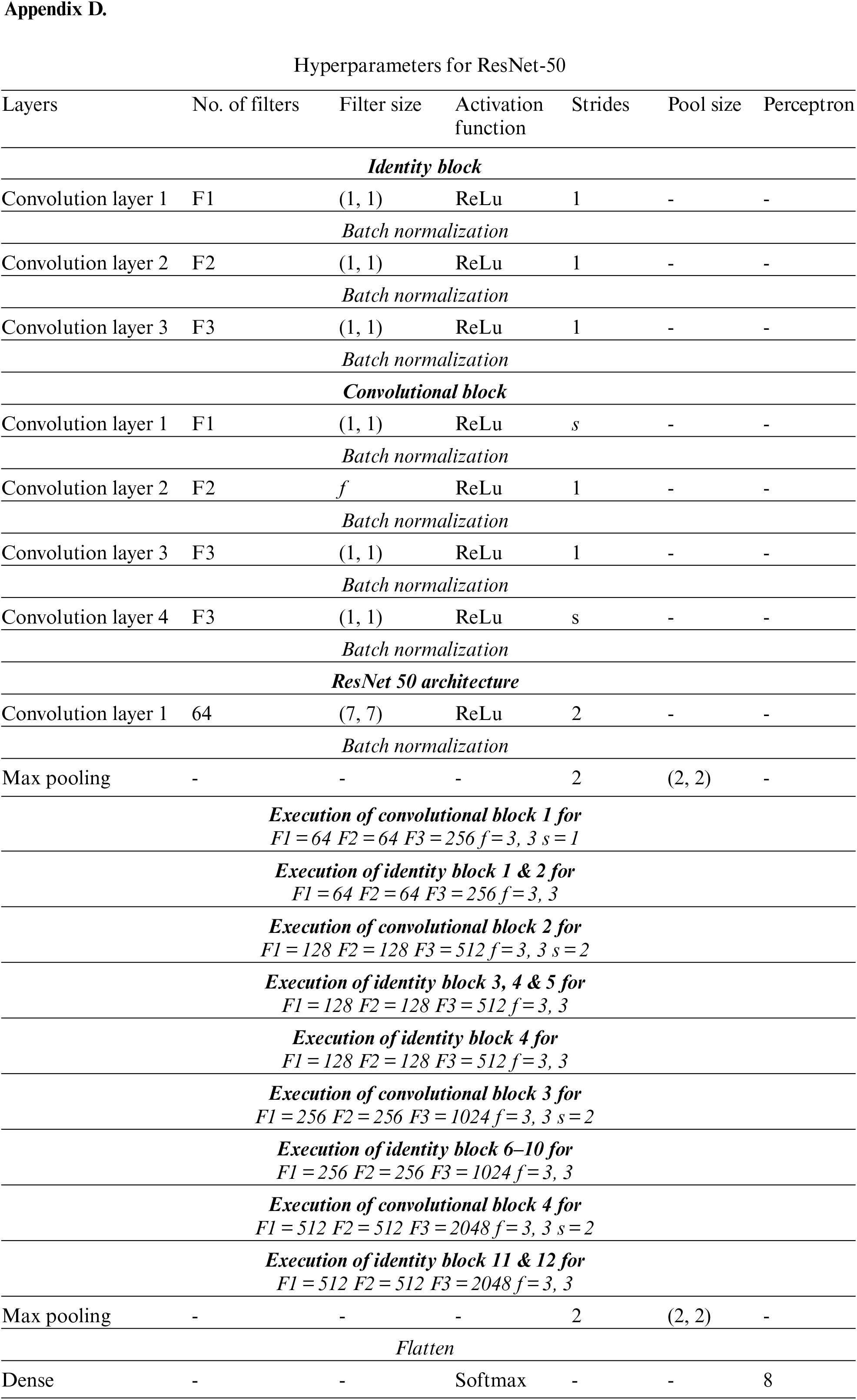
ResNet is a CNN model that was developed to mitigate the issue of vanishing gradients [35]. The key development is it introduces something called the identity shortcut connection which just skips a bunch of layers [36]. It can be seen as a special case of the Highway Network. ResNet Introduces a hyper-parameter called cardinality to adjust the model capacity and uses the split-transform-merge paradigm from the Inception model [37]. XResNet applies a number of tricks that modify things like the training or model. Heuristics to increase the parallelism of training and decrease the computational cost through lower precision computing and modifying the learning rate or biases.

Tweaking the models by modifying the network architecture is available. They explore several modifications they call ResNet A, ResNet B, ResNet C and ResNet D. These modify the stride length in particular convolutional layers. Training refinements assist in improving accuracy [35–37]. ResNet-50 is a residual network where the number ‘50’ designates the no. layers involved in training. It is a subcategory of CNNs and is widely employed for the classification of images. The standard ResNet architecture is shown in Fig. 6. Skipping connections is the novelty of ResNet [38]. Without any hyper-parameters tuning, deep-oriented nets usually suffer through vanishing gradients as the algorithm takes back-propagation, the gradient reduces. A smaller gradient makes inflexible training. The identity function would be learned by the algorithm and allows the passing of the input features over the blocks without passing over the remaining weighted layers [39]. This makes the stacking of extra layers and the network becomes deeper and deeper. Due to this vanishing gradient offsets by skipping the layers. Increasing the number of layers increases the nonlinearity of the neural network. That means, the problem becomes increasingly non-convex with an increasing number of layers. Highly non-convex planes are difficult to optimize and hence, the optimization algorithm will fail to find good minima. Residual Neural Networks solve this problem by introducing the idea of skip connections. ResNet introduces residual associates amongst layers, making the outcome of each layer a convolution of corresponding input along with its non-convolutional input [40]. Furthermore, Batch Normalization is also used in the ResNet and incorporated into VGG architecture also. ResNet-50 is usually trained for big data, i.e., volume of which is measured in billion. The network consists of multiple layers and classifies images into different classes such as nose, notch, crater, flank wear, etc. Residual Network is popularly regarded as an efficient framework for training deep neural networks. Similar to a general Deep learning algorithm, the layers signify the nonlinear process of data for extracting features and transforming them to higher dimensions or lower dimensions. It also comprises a hidden layer of traditional ANN and an array of proposed formulae. Generally, in a deep CNN, stacking of layers can be found. The specialty of this net is that it learns features at several levels such as high/mid/low at the end of each layer. Also, in residual learning, as an alternative to trying to learn features, learning from some residual is desired. The concept of Residual is nothing but the deduction of learned features from non-learned features of a particular layer. ResNet makes it happen by shortcut connections, i.e., by connecting the Nth layer to (N+X)th layer directly. It is evident that training of such nets is simpler than conventional CNNs with superior accuracy [35–40].

Figure 6: Basic architecture of ResNet [34]

4.4 VGG-16

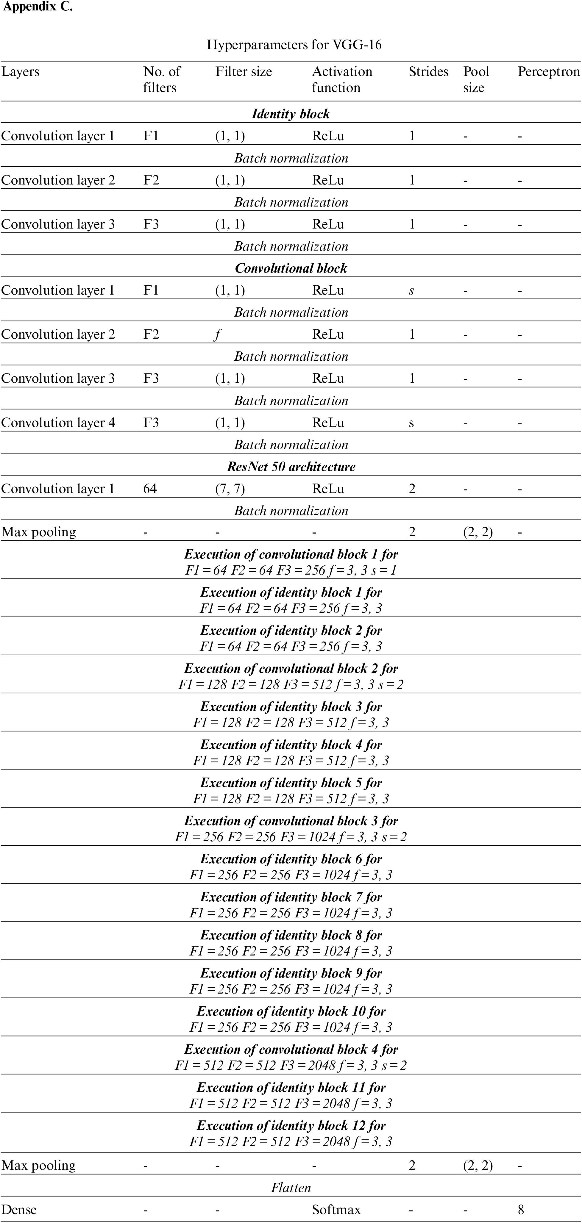
The Visual Geometry Group (VGG) of the Department of Engineering Sciences at the University of Oxford designed the VGG-16 which is nothing but a novel trained Convolutional Neural Network architecture [40]. All the CNNs have more or less similar architecture, a stack of convolution and pooling layers at the start and ending with fully connected and soft-max layers. The ‘VGG-16 Neural Network’ was particularly trained for more than a million types of images with respect to the database of the ‘ImageNet’ and or the ‘ImageNet’ database respectively, where the network consists of various types of layers, and to be specific, there were 16 layers. The modification between the ‘VGG-16’ and the ‘VGG-19’ is that this type of network is 16 layers deep and that type of network was 19 layers deep respectively [41,42]. The ‘VGG Neural Net’ was firstly presented by ‘Zisserman’ and ‘Simonyan’ in 2014 and was hence published in one of the research papers which was namely, ‘Large-Scale Image Recognition using Deep CNN’ and was first published in this paper respectively. VGG-16 is just one of the configurations that won the 2014 ImageNet challenge in localization and classification tasks. 16 indicate that the network has 16 weight layers as shown in Fig. 7. VGG secures 1st and 2nd rank for the task of localizing and classifying for 2014’s challenge of ImageNet. All the CNNs have more or less similar architecture, the stack of convolution and pooling layers at the start and ending with fully connected and soft-max layers. The major role of VGG is to enhance accuracy by addition of depth of CNN despite smaller reception slices in earlier layers while performing the task of classifying/localizing images.

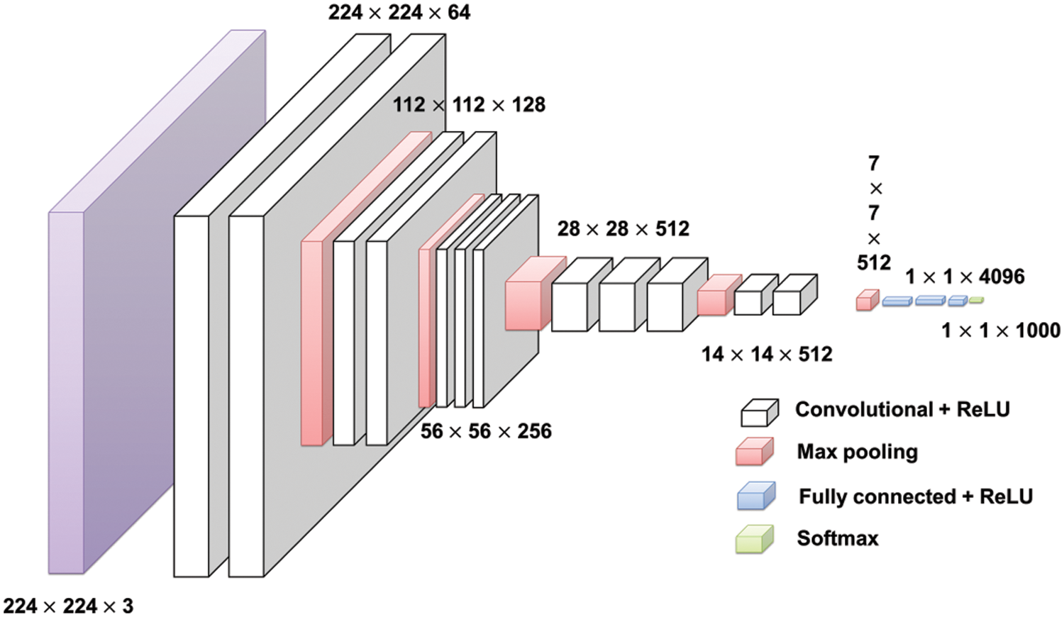
Figure 7: Basic architecture of VGG-16 [43]

Nets previous to VGG were bigger reception slices, i.e., 11×11 and 7×7 in comparison with 3×3; however, are not as deeper as VGG. Some variants of VGG exist according to a number of weighted layers for example VGG 19. Suppose the input given to VGG 19 is 224×224 RGB image and the expected output is the probability value for each of 1000 classes of the ImageNet database. In this net, the Softmax layer creates an outcome by an application function named ‘softmax’ as an activation function from the total input features received from the preceding layer. This function ‘softmax’ compresses the outcome of every unit between 1 and 0, very similar to function ‘sigmoid’. However, it also splits each outcome in a way that the total summation of the outcomes is 1. The outcome of this function is corresponding to discrete probability distributions and estimates the probability of true classes. Softmax is used in deep neural networks as an activation function at the output node. Maximum pooling put on pooling at maximum extent over its input features. Pooling is an operation in ConvNets, which combines the outcomes of a cluster of neurons at a single layer into one neuron in a succeeding layer. Maximum pooling analyzes every cluster of neurons at a previous layer and selects the maximum value from it. The application of VGG-16 is explained here. Suppose there is image data and the objective is to find the labels. The input to the network is an image of 224×224×3 sizes and there are 1000 images. There were convolutions (size 3×3) layers, max pooling (size 2×2) layers, and fully connected 16 layers at the end to make the size of the model size 528 MB. The 1st recommendation was to keep the size of all filters equal to 3×3; max pooling must be located after every 2 convolutions and filters number must be twice after every max-pooling. These recommendations were used to design the VGG-16 model for the current application [44].

5  Design and Training of Architectures Based on Spectrogram Images

CNN architectures (AlexNet, ResNet-50, LeNet-5, and VGG-16) under consideration were trained based on real-time spindle vibrations transformed as spectrogram images in order to develop a classification model for different tool configurations.

•   The dataset consisted of 100 images of each of the 8 tool configurations, i.e., in a total of 800 images. A total of 800 images were fed in different splits to each of the architecture. The splits range from 60% to 90% with the step of 10%. All four architectures were designed using the training set of split 60%, 70%, 80%, and 90% of 800 images.

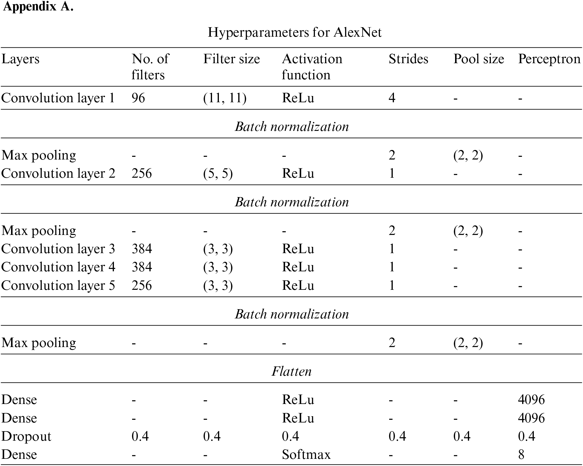
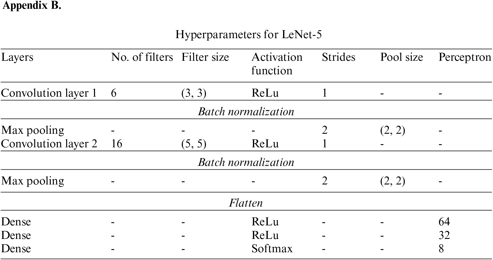
•   The hyper-parameters and architecture are given in Appendix A, B, C, and D respectively for all four architectures. The layers include convolution, max pooling, dense, and dropout. Other parameters are no. of filters, filter size, strides pool size, and perceptron. The activation function was ReLu and Softmax.

•   The activation function keeps the outcome constrained to a specific kind and adds non-linearity to data. The most popular functions are Gelu, Selu, Softsign, Softplus, Hyperbolic Tangent (tanh), Softmax, ELU, Sigmoid, Relu, etc. Sigmoid is usually employed for two-class categorization and can entail the problem of gradient vanishing. Further, it is not concentrated around zero and computation is very costlier. The tanh also causes the vanishing gradient problem. Swish, on the other hand, does not entail the problem of gradient vanishing and is established to be slightly superior to Relu however computation is complex. Relu is a better choice over Softplus and Softsign also. Relu is preferred for hidden layers. In the case of deep nets, the swish function works superior to Relu. Softmax Function is usually employed for multiple class categorizations and is thus located at the end nets. In the case of regression, a linear function is used at the end layer; for two class categorizations, sigmoid is the correct selection and for multiple class categorizations, softmax is the right choice [44]. As this research investigates multiclass classification and the hidden layers are also used in the model. So ReLu and Softmax activation functions are used.

•   Firstly, 60% of total images were employed to train all architectures. The trained model was then tested using 40% of the remaining data. Secondly, 70% of the total images were used for training all four architectures and tested using 30% of the remaining data. Thirdly, 80% of the total images were used for training all four architectures and tested using the remaining 20% of the remaining data. Lastly, 90% of the total images were used for training all four architectures and tested using 10% of the remaining data. The number of epochs varied from 10 to 50.

In the subsequent section, classification using spectrogram images has been discussed.

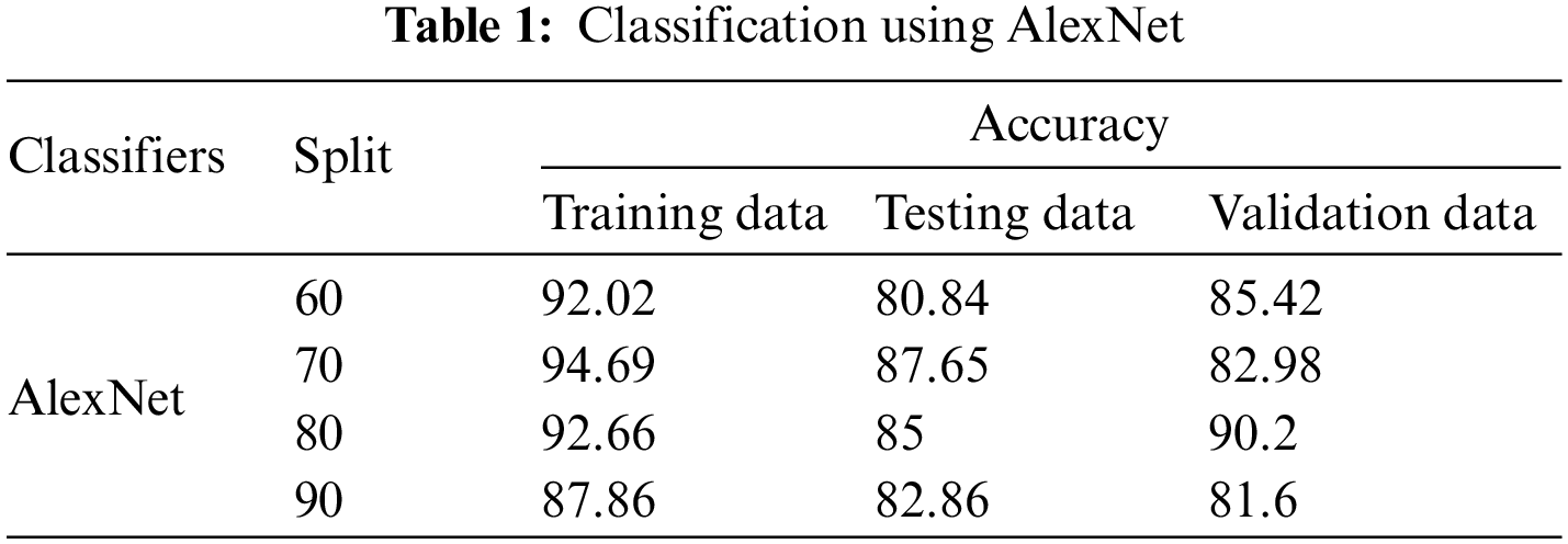
While developing the AlexNet model, as shown in Table 1, the training was carried out using different splits as explained above. The highest accuracy of each split was found when the epoch was kept at 40. For training, the highest accuracy was obtained at a 70/30 split which was 94.69% and the lowest accuracy was achieved at a 90/10 split which was 87.86%. Since AlexNet split into two networks while training and trained in two GPUs since it was too large for a single GPU to handle the network. Thus for testing data, the highest accuracy was obtained at a 70/30 split which was 87.65% and the lowest accuracy was obtained at a 60/40 split which was 80.84%. For classifying blind data, the highest accuracy was obtained at 80/20 split which was 90.2% and the lowest accuracy was obtained at 90/10 split which was 81.6%. This shows that the average accuracy of classification was 86.98%. This shows no overfitting problem as AlexNet has nearly 60 million parameters where ‘Dropout’ &‘Data augmentation’ takes care of overfitting.

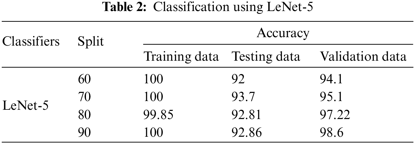
For the LeNet-5 algorithm, the highest accuracy of each split was found when the epoch was 50. It shows that for LeNet-5 from Table 2, with respect to training, the highest accuracy was obtained at 60/40, 70/30 and 90/10 split which was 100%, and the lowest accuracy was achieved at 80/20 split which was 99.85%. Within just two convolution layers and two pooling layers followed by dense layers, the architecture overfits as the accuracy of training for all splits is almost 100%. Owing to the overfitting of the model in training, testing accuracy drops to 92%–93%. While classifying blind data, the highest accuracy was obtained at the 90/10 split which was 98.6% and the lowest accuracy was obtained at the 60/40 split which was 94.1%.

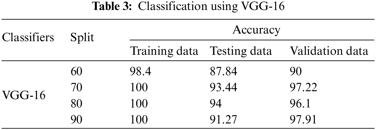
In the case of VGG-16, the highest accuracy of each split was found when the epoch was 20. It is apparent from Table 3, as there are 19 different layers; this model also overfits in training as accuracy is almost 100%. This overfitting in training drops testing accuracy to 87%–94%. For testing data, the highest accuracy was obtained at 80/20 split which was 94% and the lowest accuracy was obtained at the 60/40 split which was 87.44%. While classifying blind data, the highest accuracy was obtained at the 90/10 split which was 97.91% and the lowest accuracy was obtained at the 60/40 split which was 90%.

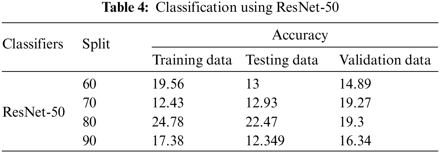
The design of the ResNet-50 model shows that the highest accuracy of each split was found when the epoch was 20. The accuracy was substantially lower than other architectures despite rigorous hyperparameter tuning as shown in Table 4. The model mitigates the issue of vanishing gradients however the identity shortcut connection just skips a bunch of layers. Even though the heuristics increases the parallelism of training and decreases the computational cost but it affects precision computing and decreases the learning rate. This can be evident from the results. Concerning training, the accuracy ranges from 12.43% to 24.78%. Owing to insufficient training, testing accuracy also drops to range from 12.349% to 22.47%. While classifying blind data, the highest accuracy was obtained at the 80/20 split which was 19.3% and the lowest accuracy was obtained at the 60/40 split which was 14.89%. Overall comparison of all models shows that the highest average accuracy of classification (96.35%) was obtained through the LeNet-5 model, followed by VGG-16 (95.51%) and AlexNet (86.98%). The performance of ResNet-50 was very poor which could not classify faults more than 17.05%. In addition to this, the design of classifiers was examined with detailed results of classification. The validation results considering the dataset are presented in the next section with the help of confusion matrices to understand correct and incorrect classification of tool health.

6  Classification Results and Discussion

The classification results, i.e., how designed CNN architecture classifies samples correctly are explained using the confusion matrix. The matrix is made up of 8 columns and 8 rows defining the actual and predicted class of tool conditions. In this section, classification results considering validation data are presented. After successful training and testing of models, for validation, out of 100 separate images that were created amongst each class, at random 36 photos were selected as the blind datasets. These 36 photos were then used to validate models trained using split 60%, 70%, 80%, and 90% and presented here. The confusion matrix for classification using AlexNet depicted in Fig. 8d 90/10 is explained as follows. There were a total of 288 samples considering all labels. For all wear tool conditions, all 36 samples were correctly classified. For the built-up edge tool condition, only 13 samples were correctly classified out of a total of 36 samples; 20 samples were misclassified as all wear, 2 samples were misclassified as crater wear and 1 sample was misclassified as edge fracture. For the next case, crater wear condition, 33 samples were correctly classified out of 36 samples; 2 were misclassified as all wear and 1 was misclassified as healthy. Similarly, other classifications can be understood.

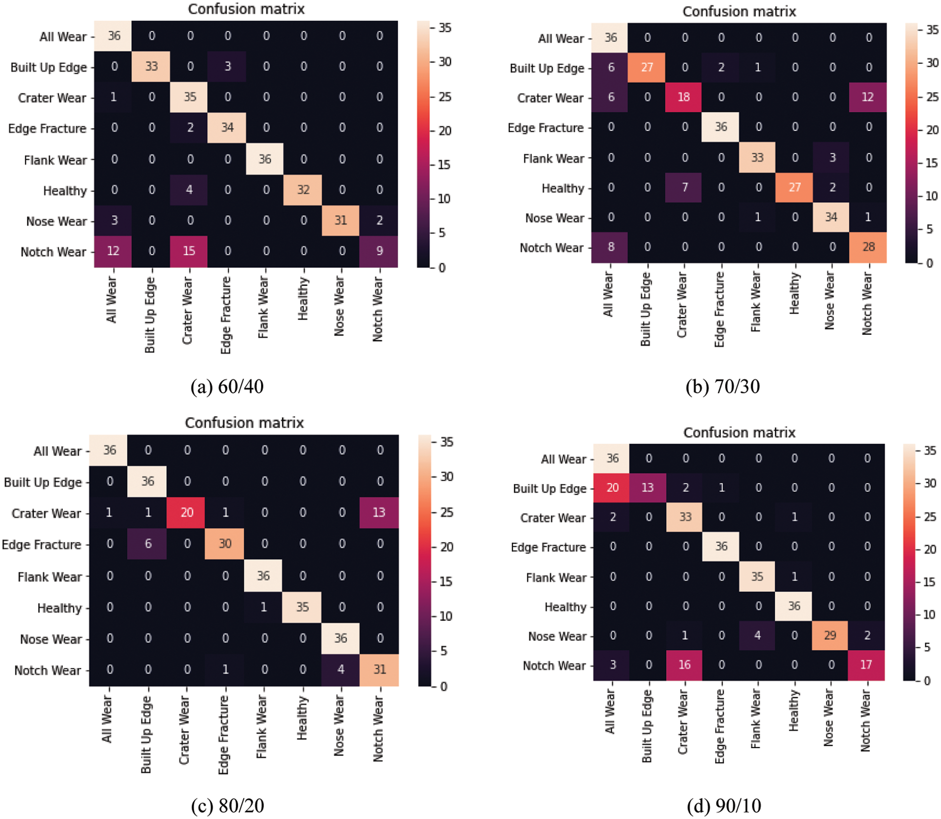
Figure 8: Confusion matrix for classification using AlexNet

The classification using LeNet-5 is depicted through confusion matrix in Figs. 9a–9d. It can be seen that the classification of samples from ‘all wear’, ‘built up edge’, ‘crater wear’, ‘edge fracture’, and ‘healthy tool’ condition does not affect much over the change of % split of train and test. However, there is considerable change in the classification of notch, nose, and flank wear. The maximum misclassification occurs for ‘notch wear’ as it arises at the line of cutting depth and rubs over the work shoulder. This rubbing worsens and approaches tool surface abrasion and affects the cutting tool chemically which perhaps affects tool condition. The results for ‘notch wear’ in classification using AlexNet are even worst as only 9 samples were correctly classified in case of a 60/40 split. The confusion matrix for VGG-16 is shown in Figs. 10a–10d. By carefully observing these matrices, the classification results for ‘notch-wear’ have been substantially improved in this case as compared to the previous case. The confusion matrix for the 80/20 split shows that 11 images were incorrectly classified and 277 images were classified accurately. Similarly, other classifications can be understood. Thus it is recommended that VGG-16 is useful to classify notch wear case as the abrasion on the tool surface is correctly recognized through multiple layers of VGG-16. Also, the classification of flank and nose wear conditions is superior to AlexNet. Overall the performance of VGG-16 and LeNet-5 is superior for all kinds of wears and is recommended for real-time implementation of these models.

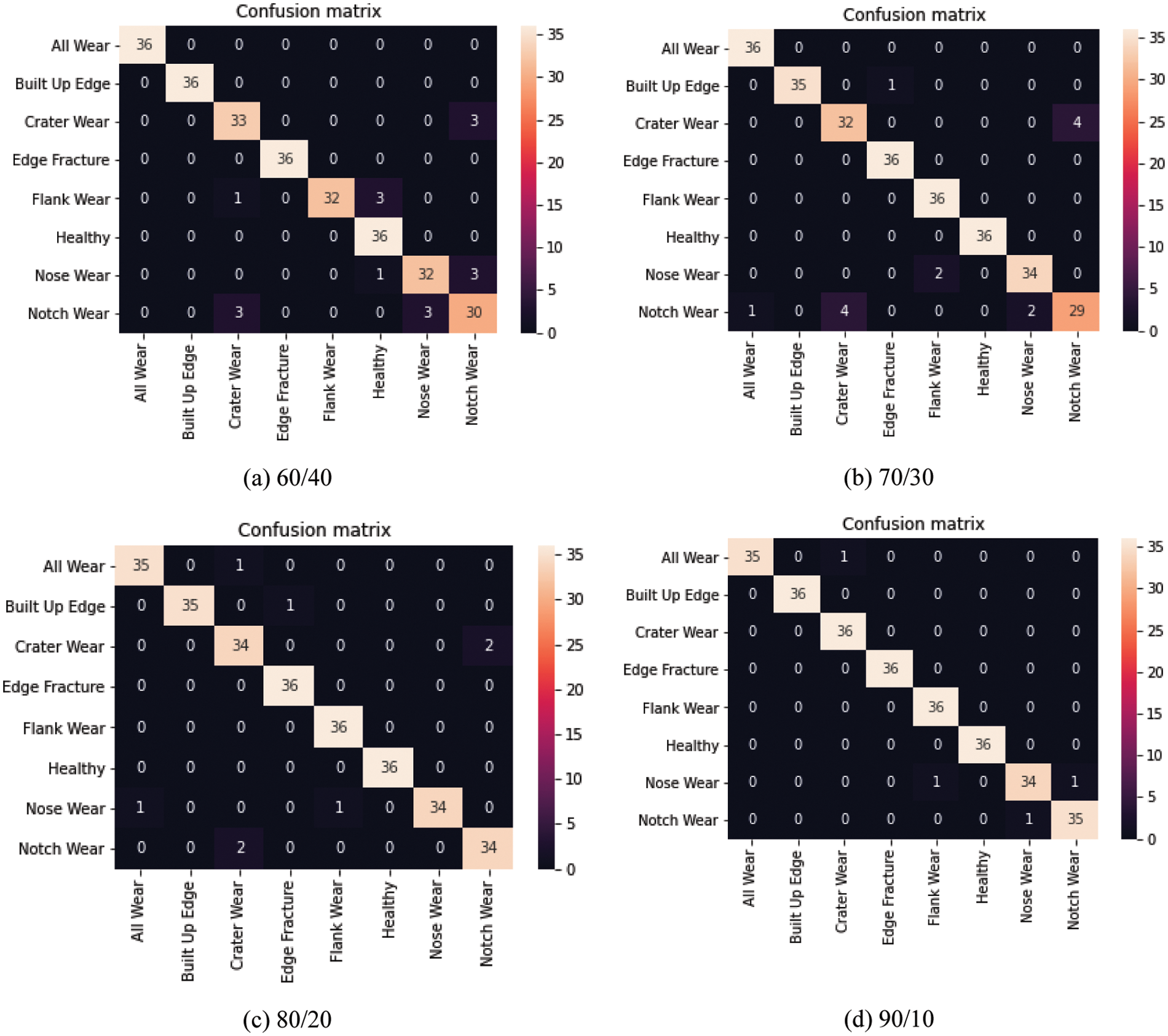
Figure 9: Confusion matrix for classification using LeNet-5

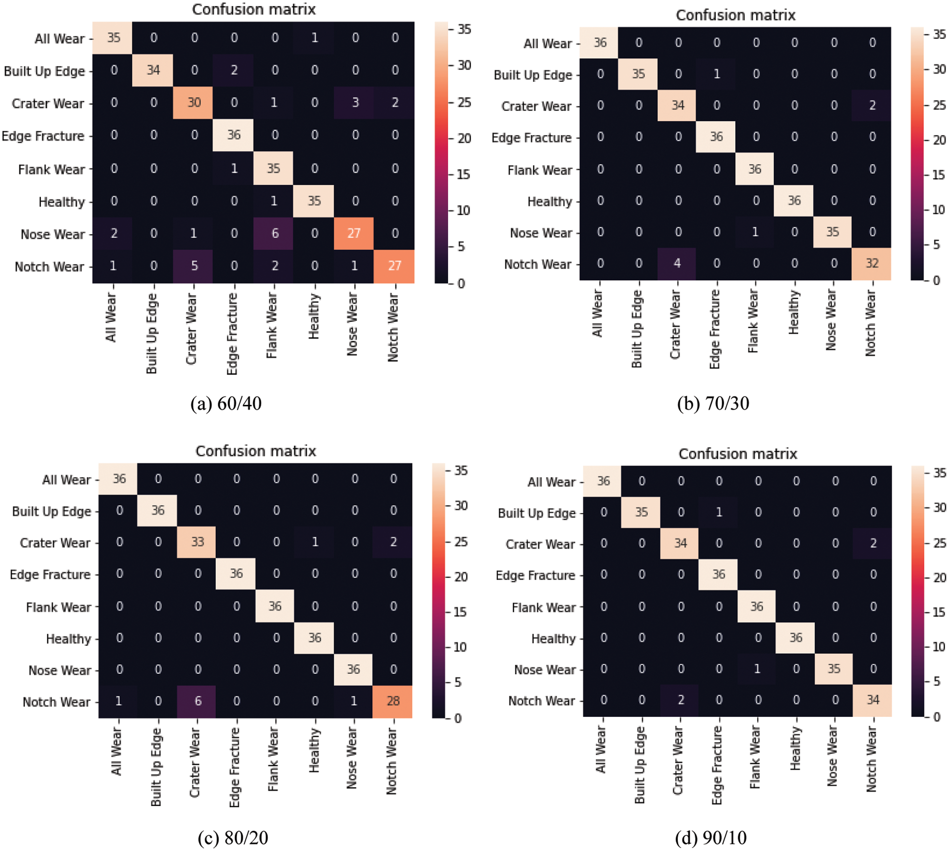
Figure 10: Confusion matrix for classification using VGG-16

7  Conclusions

The use of deep learning-based techniques for mapping vibration response to the corresponding cutting tool condition has been successfully demonstrated from image-based data classification. The results obtained show that this methodology can effectively classify tool health conditions. Time-frequency vibrations response was observed for 8 different tool wears and has facilitated suitable tool condition classification. The CNN architecture-based classification methodology can be employed for the ideal use of cutting tools during manufacturing processes, to reduce idle times during manufacturing, and much more. The classification results achieved considering training, testing and blindfolds indicate that the methodology is proficient in tool health monitoring. Though the AlexNet model offers an accuracy of more than 85%, there is misclassification amongst faulty classes. This can be eliminated by considering the VGG-16 and LeNet-5 models where there was the least misclassification of flank, nose, and notch wear. The VGG-16 alone is sufficient to classify notch wear clearly. Overall the performance of VGG-16 and LeNet-5 is superior for all kinds of wears and thus recommended for real-time implementation of these models. Manual feature extraction was successfully eliminated with the help of this new deep network technology since manual feature extraction increases the computational time and complexity of the system. This system shall assist edge-old systems in up grading to be smarter with fewer resources. This scheme shall ensure the effective use of the cutting tool. The aforesaid strategies will be investigated in future research to decrease the amount of experimental effort necessary. It would be feasible to eliminate the requirement for data augmentation with a larger and more comprehensive dataset. This might also help with the development of a more precise classifier. Additionally, future research should be directed toward the deployment and real-time implementation of this methodology in the industry. With the recent advancements in MEMS-based sensors and instrumentation, the cost of data collection through experimentation has significantly reduced. For the case of measuring vibrations, MEMS-based accelerometers such as ADXL335/ADXL345 can be integrated with open source hardware such as Arduino/Raspberry Pi, and data can be stored/processed/displayed via Python/MS-Excel.

Funding Statement: The authors received no specific funding for this study.

Conflicts of Interest: The authors declare that they have no conflicts of interest to report regarding the present study.

References

 1.  Patange, A. D., Jegadeeshwaran, R. (2020). Application of Bayesian family classifiers for cutting tool inserts health monitoring on CNC milling. International Journal of Prognostics and Health Management, 11(2). DOI 10.36001/ijphm.2020.v11i2.2929. [Google Scholar] [CrossRef]

 2.  Patange, A. D., Jegadeeshwaran, R. (2021). Review on tool condition classification in milling: A machine learning approach. Materials Today: Proceedings, 46(2), 1106–1115. [Google Scholar]

 3.  Liu, B., Li, H., Ou, J., Wang, Z., Sun, W. (2022). Intelligent recognition of milling tool wear status based on variational auto-encoder and extreme learning machine. The International Journal of Advanced Manufacturing Technology, 119, 4109–4123. DOI 10.1007/s00170-021-08427-y. [Google Scholar] [CrossRef]

 4.  Sun, H., Zhang, J., Mo, R., Zhang, X. (2020). In-process tool condition forecasting based on a deep learning method. Robotics and Computer-Integrated Manufacturing, 64, 101924. DOI 10.1016/j.rcim.2019.101924. [Google Scholar] [CrossRef]

 5.  Shi, C., Panoutsos, G., Luo, B., Liu, H., Li, B. et al. (2018). Using multiple-feature-spaces-based deep learning for tool condition monitoring in ultra-precision manufacturing. IEEE Transactions on Industrial Electronics, 66(5), 3794–3803. DOI 10.1109/TIE.2018.2856193. [Google Scholar] [CrossRef]

 6.  Cheng, C., Li, J., Liu, Y., Nie, M., Wang, W. (2019). Deep convolutional neural network-based in-process tool condition monitoring in abrasive belt grinding. Computers in Industry, 106, 1–13. DOI 10.1016/j.compind.2018.12.002. [Google Scholar] [CrossRef]

 7.  Lee, C. H., Jwo, J. S., Hsieh, H. Y., Lin, C. S. (2020). An intelligent system for grinding wheel condition monitoring based on machining sound and deep learning. IEEE Access, 8, 58279–58289. DOI 10.1109/Access.6287639. [Google Scholar] [CrossRef]

 8.  Qiao, H., Wang, T., Wang, P. (2020). A tool wear monitoring and prediction system based on multiscale deep learning models and fog computing. The International Journal of Advanced Manufacturing Technology, 108(7), 2367–2384. DOI 10.1007/s00170-020-05548-8. [Google Scholar] [CrossRef]

 9.  He, Z., Shi, T., Xuan, J., Li, T. (2021). Research on tool wear prediction based on temperature signals and deep learning. Wear, 478–479, 203902. DOI 10.1016/j.wear.2021.203902. [Google Scholar] [CrossRef]

10. Zhou, Y., Zhi, G., Chen, W., Qian, Q., He, D. et al. (2022). A new tool wear condition monitoring method based on deep learning under small samples. Measurement, 189, 110622. DOI 10.1016/j.measurement.2021.110622. [Google Scholar] [CrossRef]

11. Xu, X., Wang, J., Ming, W., Chen, M., An, Q. (2021). In-process tap tool wear monitoring and prediction using a novel model based on deep learning. The International Journal of Advanced Manufacturing Technology, 112(1), 453–466. DOI 10.1007/s00170-020-06354-y. [Google Scholar] [CrossRef]

12. Cheng, M., Jiao, L., Yan, P., Jiang, H., Wang, R. et al. (2022). Intelligent tool wear monitoring and multi-step prediction based on deep learning model. Journal of Manufacturing Systems, 62, 286–300. DOI 10.1016/j.jmsy.2021.12.002. [Google Scholar] [CrossRef]

13. Fernandes, T. E., Ferreira, M. A., de Miranda, G. P., Dutra, A. F., Antunes, M. P. et al. (2022). Classification of lathe’s cutting tool wear based on an autonomous machine learning model. Journal of Control, Automation and Electrical Systems, 33(1), 167–182. DOI 10.1007/s40313-021-00819-5. [Google Scholar] [CrossRef]

14. Kumar, D. P., Muralidharan, V., Ravikumar, S. (2022). Histogram as features for fault detection of multi point cutting tool–A data driven approach. Applied Acoustics, 186, 108456. DOI 10.1016/j.apacoust.2021.108456. [Google Scholar] [CrossRef]

15. Stuhr, B., Liu, R. (2022). A flexible similarity-based algorithm for tool condition monitoring. Journal of Manufacturing Science and Engineering, 144(3), 031010. DOI 10.1115/1.4051885. [Google Scholar] [CrossRef]

16. You, Z., Gao, H., Li, S., Guo, L., Liu, Y. et al. (2022). Multiple activation functions and data augmentation based light weight network for in-situ tool condition monitoring. IEEE Transactions on Industrial Electronics, 69(12), 13656–13664. DOI 10.1109/TIE.2021.3139202. [Google Scholar] [CrossRef]

17. Li, X. Q., Song, L. K., Bai, G. C. (2021). Recent advances in reliability analysis of aeroengine rotor system: A review. International Journal of Structural Integrity, 13(1), 1–29. DOI 10.1108/IJSI-10-2021-0111. [Google Scholar] [CrossRef]

18. Cherid, D., Bourahla, N., Laghoub, M. S., Mohabeddine, A. (2021). Sensor number and placement optimization for detection and localization of damage in a suspension bridge using a hybrid ANN-PCA reduced FRF method. International Journal of Structural Integrity, 13(1), 133–149. DOI 10.1108/IJSI-07-2021-0075. [Google Scholar] [CrossRef]

19. Luo, C., Keshtegar, B., Zhu, S. P., Taylan, O., Niu, X. P. (2022). Hybrid enhanced Monte Carlo simulation coupled with advanced machine learning approach for accurate and efficient structural reliability analysis. Computer Methods in Applied Mechanics and Engineering, 388, 114218. DOI 10.1016/j.cma.2021.114218. [Google Scholar] [CrossRef]

20. Lin, Y. R., Lee, C. H., Lu, M. C. (2022). Robust tool wear monitoring system development by sensors and feature fusion. Asian Journal of Control, 24(3), 1005–1021. DOI 10.1002/asjc.2741. [Google Scholar] [CrossRef]

21. Kom–Guide (2016). Technical manual drilling, threading, reaming, milling. Komet Group. https://www.yumpu.com/en/document/view/3876114/komguide-technical-manual-komet-group. [Google Scholar]

22. Zhao, N., Zhang, J., Ma, W., Jiang, Z., Mao, Z. (2022). Variational time-domain decomposition of reciprocating machine multi-impact vibration signals. Mechanical Systems and Signal Processing, 172, 108977. DOI 10.1016/j.ymssp.2022.108977. [Google Scholar] [CrossRef]

23. Komorska, I., Puchalski, A. (2021). Rotating machinery diagnosing in non-stationary conditions with empirical mode decomposition-based wavelet leaders multifractal spectra. Sensors, 21(22), 7677. DOI 10.3390/s21227677. [Google Scholar] [CrossRef]

24. Lu, L., Ren, W. X., Wang, S. D. (2022). Fractional fourier transform: Time-frequency representation and structural instantaneous frequency identification. Mechanical Systems and Signal Processing, 178, 109305. DOI 10.1016/j.ymssp.2022.109305. [Google Scholar] [CrossRef]

25. Xin, G., Li, Z., Jia, L., Zhong, Q., Dong, H. et al. (2021). Fault diagnosis of wheelset bearings in high-speed trains using logarithmic short-time Fourier transform and modified self-calibrated residual network. IEEE Transactions on Industrial Informatics, 18(10), 7285–7295. DOI 10.1109/TII.2021.3136144. [Google Scholar] [CrossRef]

26. Mokrzan, D., Szymański, G. M. (2021). Time-frequency methods for processing non-stationary diagnostic vibroacoustic signals. Rail Vehicles/Pojazdy Szynowe, (3), 44–57. DOI 10.53502/RAIL-143047. [Google Scholar] [CrossRef]

27. Manhertz, G., Bereczky, A. (2021). STFT spectrogram based hybrid evaluation method for rotating machine transient vibration analysis. Mechanical Systems and Signal Processing, 154, 107583. DOI 10.1016/j.ymssp.2020.107583. [Google Scholar] [CrossRef]

28. LeCun, Y., Bottou, L., Bengio, Y., Haffner, P. (1998). Gradient-based learning applied to document recognition. Proceedings of the IEEE, 86(11), 2278–2324. [Google Scholar]

29. Zhu, Y., Li, G., Wang, R., Tang, S., Su, H. et al. (2021). Intelligent fault diagnosis of hydraulic piston pump combining improved LeNet-5 and PSO hyperparameter optimization. Applied Acoustics, 183, 108336. DOI 10.1016/j.apacoust.2021.108336. [Google Scholar] [CrossRef]

30. Zaibi, A., Ladgham, A., Sakly, A. (2021). A lightweight model for traffic sign classification based on enhanced LeNet-5 network. Journal of Sensors, 2021, 8870529. DOI 10.1155/2021/8870529. [Google Scholar] [CrossRef]

31. Gonzalez, T. F. (2007). AlexNet. In: Handbook of approximation algorithms and metaheuristics. New York: Chapman and Hall/CRC. DOI 10.1201/9781420010749. [Google Scholar] [CrossRef]

32. Alom, M. Z., Taha, T. M., Yakopcic, C., Westberg, S., Sidike, P. et al. (2018). The history began from AlexNet: A comprehensive survey on deep learning approaches. arXiv preprint arXiv:1803.01164. [Google Scholar]

33. Krizhevsky, A., Sutskever, I., Hinton, G. E. (2012). Imagenet classification with deep convolutional neural networks. Advances in Neural Information Processing Systems, 60(6), 84–90. [Google Scholar]

34. Mehrotra, R., Ansari, M. A., Agrawal, R., Anand, R. S. (2020). A transfer learning approach for AI-based classification of brain tumors. Machine Learning with Applications, 2, 100003. DOI 10.1016/j.mlwa.2020.100003. [Google Scholar] [CrossRef]

35. Feng, V. (2017). An overview of ResNet and its variants. Towards Data Science. https://towardsdatascience.com/understanding-resnet-and-its-variants-719e5b8d2298. [Google Scholar]

36. Li, S., Jiao, J., Han, Y., Weissman, T. (2016). Demystifying ResNet. arXiv preprint arXiv:1611.01186. [Google Scholar]

37. He, K., Zhang, X., Ren, S., Sun, J. (2016). Identity mappings in deep residual networks. arXiv preprint arXiv:1603.05027. [Google Scholar]

38. Zhang, X., Zou, J., He, K., Sun, J. (2015). Accelerating very deep convolutional networks for classification and detection. IEEE Transactions on Pattern Analysis and Machine Intelligence, 38(10), 1943–1955. DOI 10.1109/TPAMI.2015.2502579. [Google Scholar] [CrossRef]

39. Ren, S., He, K., Girshick, R., Sun, J. (2015). Faster R-CNN: Towards real-time object detection with region proposal networks. arXiv preprint arXiv:1506.01497. [Google Scholar]

40. Wu, J., Leng, C., Wang, Y., Hu, Q., Cheng, J. (2016). Quantized convolutional neural networks for mobile devices. arXiv preprint arXiv:1512.06473. [Google Scholar]

41. Patange, A. D., Jegadeeshwaran, R. (2021). A machine learning approach for vibration-based multipoint tool insert health prediction on vertical machining centre (VMC). Measurement, 173, 108649. DOI 10.1016/j.measurement.2020.108649. [Google Scholar] [CrossRef]

42. Khade, H. S., Patange, A. D., Pardeshi, S. S., Jegadeeshwaran, R. (2021). Design of bagged tree ensemble for carbide coated inserts fault diagnosis. Materials Today: Proceedings, 46(2), 1283–1289. [Google Scholar]

43. Patange, A. D., Jegadeeshwaran, R., Bajaj, N. S., Khairnar, A. N., Gavade, N. A. (2022). Application of machine learning for tool condition monitoring in turning. Sound & Vibration, 56(2), 127–145. DOI 10.32604/sv.2022.014910. [Google Scholar] [CrossRef]

44. Ul Hassan, M. (2018). VGG16-convolutional network for classification and detection. Neurohive. https://neurohive.io/en/popular-networks/vgg16/. [Google Scholar]

Appendix A.

Appendix B.

Appendix C.

Appendix D.