On the Mean Value of High-Powers of a Special Character Sum Modulo a Prime

Xiaodan Yuan; Wenpeng Zhang

doi:10.32604/cmes.2023.024363

icon Open Access

ARTICLE

On the Mean Value of High-Powers of a Special Character Sum Modulo a Prime

Xiaodan Yuan^*, Wenpeng Zhang

School of Mathematics, Northwest University, Xi’an, China

* Corresponding Author: Xiaodan Yuan. Email: email

(This article belongs to the Special Issue: Application of Computer Tools in the Study of Mathematical Problems)

Computer Modeling in Engineering & Sciences 2023, 136(1), 943-953. https://doi.org/10.32604/cmes.2023.024363

Received 29 May 2022; Accepted 07 September 2022; Issue published 05 January 2023

Abstract

In this paper, we use the elementary methods, the properties of Dirichlet character sums and the classical Gauss sums to study the estimation of the mean value of high-powers for a special character sum modulo a prime, and derive an exact computational formula. It can be conveniently programmed by the “Mathematica” software, by which we can get the exact results easily.

Keywords

Quadratic character; the classical gauss sums; the mean value of high-power; computational formula

1 Introduction

Let p be an odd prime, the quadratic character modulo p is called the Legendre symbol, which is defined by

$(ap)={1,ifaisaquadraticresiduemodulop;−1,ifaisaquadraticnon-residuemodulop;0,ifp∣a.$

Many mathematicians have studied the properties of the Legendre symbol and obtained a series of important results (see [1–13]). Perhaps the most representative properties of the Legendre’s symbol are as follows:

Let p and q be two distinct odd primes, then one has the quadratic reciprocal formula (see [14]: Theorem 9.8 or [15]: Theorems 4–6)

$(pq)⋅(qp)=(−1)(p−1)(q−1)4.$

For any odd prime p with $p≡1 mod 4$ , there exists two non-zero integers $αp$ and $βp$ such that (see [15]: Theorems 4–11)

$p=αp2+βp2.$ (1)

In fact, the integers $αp$ and $βp$ in Eq. (1) can be represented by the Jacobsthal sums $ϕ2(r)$ , which is (see [16]: Definition of the Jacobsthal sums)

$ϕk(r)=∑a=1p−1(ap)(ak+rp)andαp=12ϕ2(1),βp=12ϕ2(s),$

where s is any quadratic non-residue modulo p.

Now we consider a sum A(r) be similar to $βp$ . For any integers r with $(r,p)=1$ and $k≥0$ , let A(r) and $Sk(p)$ be defined as follows:

$A(r)=1+∑a=1p−1(a2+ra¯p)andSk(p)=1p−1∑r=1p−1Ak(r).$

In this paper, we give an exact computational formula for $Sk(p)$ with $p≡1 mod 6$ , and prove the following result:

Theorem. Let p be a prime with $p≡1 mod 6$ , for any integer k, we have the identity

$Sk(p)=13⋅[dk+(−d+9b2)k+(−d−9b2)k],$

where d and b are uniquely determined by $4p=d2+27b2$ , $d≡1 mod 3$ and $b>0$ .

From this Theorem, we can immediately deduce the following four Corollaries:

Corollary 1. Let p be a prime with $p≡1 mod 6$ , then we have

$1p−1∑r=1p−111+∑a=1p−1(a2+ra¯p)=1p−1∑r=1p−111+∑a=1p−1(a4+rap)=pd⋅(3p−d2).$

Corollary 2. Let p be a prime with $p≡1 mod 6$ , we have

$1p−1∑r=1p−11[1+∑a=1p−1(a2+ra¯p)]2=1p−1∑r=1p−11[1+∑a=1p−1(a4+rap)]2=3⋅p2d2⋅(3p−d2)2.$

Corollary 3. Let p be a prime with $p≡1 mod 6$ , then we have

$1p−1∑r=1p−1[1+∑a=1p−1(a2+ra¯p)]4=1p−1∑r=1p−1[1+∑a=1p−1(a4+rap)]4=6⋅p2.$

Corollary 4. Let p be a prime with $p≡1 mod 6$ , we have

$1p−1∑r=1p−1[1+∑a=1p−1(a2+ra¯p)]6=1p−1∑r=1p−1[1+∑a=1p−1(a4+rap)]6=18p3+d2⋅(d2−3p)2.$

Some notes: In our Theorem, we only discuss the case $p≡1 mod 6$ . If $p≡5 mod 6$ , the result is trivial, see Proposition 6.1.2 in [16]. In this case, for any integer r with $(r,p)=1$ , we have the identity

$A(r)=1+∑a=1p−1(a2+ra¯p)=1+∑a=1p−1(a3p)(a3+rp)=1+∑a=1p−1(1+ra¯p)=∑a=0p−1(1+rap)=0.$

Thus, for all prime p with $p≡5 mod 6$ and $k≥1$ , we have $Sk(p)=0$ .

In addition, our Theorem holds for all negative integers.

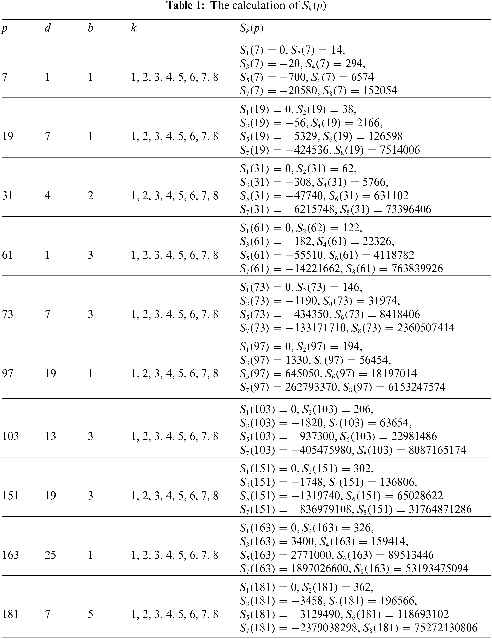
Obviously, the advantage of our work is that it can transfer a complex mathematical computational problem into a simple form suitable for computer programming. It means that for any fixed prime p with $p≡1 mod 6$ and integer k, the exact value of $Sk(p)$ can be calculated by our Theorem and a simple computer program. In Section 4, we give an example to calculate the exact results of the prime number p within 200 satisfying conditions $p≡1 mod 6$ and $d≡1 mod 3$ . The exact results of calculation are summarised in Table 1.

images

2 Several Lemmas

In this section, we give some simple Lemmas, which are necessary in the proofs of our Theorem. In addition, we need some properties of the classical Gauss sums and character sums, which can be found in many number theory books, such as [14,15] or [17], and we will not repeat them. First, we have the following:

Lemma 1. Let p be a prime with $p≡1 mod 3$ , for any third-order character $λ$ modulo p, we have the identity

$τ3(λ)+τ3(λ¯)=dp,$

where $τ(χ)=∑a=1p−1χ(a)e(ap)$ denotes the classical Gauss sums with $e(y)=e2πiy$ and $i2=−1$ , d is the same as the one in the Theorem.

Proof. See references [18] or [19].

Lemma 2. Let p be an odd prime, for any non-principal character $χ$ modulo p, we have the identity

$τ(χ2)=χ2(2)τ(χ2)⋅τ(χ)⋅τ(χχ2),$

where $χ2=(∗p)$ denotes the Legendre’s symbol modulo p.

Proof. From the properties of the classical Gauss sums we have

$∑a=0p−1χ(a2−1)=∑a=0p−1χ((a+1)2−1)=∑a=1p−1χ(a)χ(a+2)=1τ(χ¯)∑b=1p−1χ¯(b)∑a=1p−1χ(a)e(b(a+2)p)=τ(χ)τ(χ¯)∑b=1p−1χ¯(b)χ¯(b)e(2bp)=τ(χ)τ(χ¯)∑b=1p−1χ¯2(b)e(2bp)=χ2(2)⋅τ(χ)⋅τ(χ¯2)τ(χ¯).$ (2)

On the other hand, for any integer b with $(b,p)=1$ , from the identity

$∑a=0p−1e(ba2p)=1+∑a=1p−1(1+χ2(a))e(bap)=∑a=1p−1χ2(a)e(bap)=χ2(b)⋅τ(χ2)$

we also have

$∑a=0p−1χ(a2−1)=1τ(χ¯)∑a=0p−1∑b=1p−1χ¯(b)e(b(a2−1)p)=1τ(χ¯)∑b=1p−1χ¯(b)e(−bp)∑a=0p−1e(ba2p)=τ(χ2)τ(χ¯)∑b=1p−1χ¯(b)χ2(b)e(−bp)=χ2(−1)χ¯(−1)τ(χ2)⋅τ(χ¯χ2)τ(χ¯).$ (3)

From Eqs. (2) and (3) we have the identity

$τ(χ¯2)=χ¯2(2)⋅χ2(−1)χ¯(−1)⋅τ(χ2)⋅τ(χ¯χ2)τ(χ)$

or

$τ(χ2)=χ2(2)τ(χ2)⋅τ(χ)⋅τ(χχ2).$

This proves Lemma 2.

Lemma 3. Let p be a prime p with $p≡1 mod 6$ , then for any integer r with $(r,p)=1$ and three order character $λ$ modulo p, we have the identity

$∑a=1p−1(a2+ra¯p)=−1+1p⋅(λ¯(2r)⋅τ3(λ)+λ(2r)⋅τ3(λ¯)).$

Proof. From the characteristic function of the cubic residue modulo p, we have

$13⋅(1+λ(a)+λ¯(a))={1ifaisacubicresiduemodulop;0otherwise.$ (4)

Applying Eq. (4) we have

$∑a=1p−1(a2+ra¯p)=∑a=1p−1χ2(a¯3)χ2(a3+r)=∑a=1p−1χ2(a3)χ2(a3+r)=∑a=1p−1(1+λ(a)+λ¯(a))χ2(a)χ2(a+r)=∑a=1p−1χ2(1+ra¯)+∑a=1p−1λ(a)χ2(a)χ2(a+r)+∑a=1p−1λ¯(a)χ2(a)χ2(a+r)=−1+λ(r)∑a=1p−1λ(a)χ2(a)χ2(a+1)+λ¯(r)∑a=1p−1λ¯(a)χ2(a)χ2(a+1).$ (5)

From the properties of the classical Gauss sums, we have

$∑a=1p−1λ(a)χ2(a)χ2(a+1)=1τ(χ2)⋅∑b=1p−1χ2(b)∑a=1p−1λ(a)χ2(a)e(b(a+1)p)=1τ(χ2)⋅τ(λχ2)⋅τ(λ¯).$ (6)

Taking $χ=λ$ in Lemma 2, we have

$τ(λ¯)=λ¯(2)τ(χ2)⋅τ(λ)⋅τ(λχ2).$ (7)

Note that $τ(λ)⋅τ(λ¯)=p$ , from Eqs. (6) and (7) we have

$∑a=1p−1λ(a)χ2(a)χ2(a+1)=λ(2)p⋅τ3(λ¯).$ (8)

Similarly, we also have

$∑a=1p−1λ¯(a)χ2(a)χ2(a+1)=λ¯(2)p⋅τ3(λ).$ (9)

Combining Eqs. (5), (8) and (9) we can deduce that

$∑a=1p−1(a2+ra¯p)=−1+1p⋅(λ¯(2r)⋅τ3(λ)+λ(2r)⋅τ3(λ¯)).$

This proves Lemma 3.

Lemma 4. Let p be any odd prime with $p≡1 mod 6$ , then for any integers $k≥3$ and r with $(r,p)=1$ , we have the third order recursive formula

$Ak(r)=3p⋅Ak−2(r)+(d3−3dp)⋅Ak−3(r),$

where d is the same as defined in the Theorem.

Proof. Note that $λ3=λ¯3=χ0$ , the principal character modulo p, from Lemma 1 and Lemma 3 we have

$A3(r)=1p3⋅(λ¯(2r)⋅τ3(λ)+λ(2r)⋅τ3(λ¯))3=1p3⋅[τ9(λ)+τ9(λ¯)+3p3⋅(λ¯(2r)⋅τ3(λ)+λ(2r)⋅τ3(λ¯))]=1p3⋅[(τ3(λ)+τ3(λ¯))3−3p3(τ3(λ)+τ3(λ¯))+3p4⋅A(r)]=d3−3dp+3p⋅A(r).$ (10)

Indeed, for any integer $k≥3$ , from Eq. (10) we have the third order recursive formula

$Ak(r)=Ak−3(r)⋅A3(r)=3p⋅Ak−2(r)+(d3−3dp)⋅Ak−3(r).$

This proves Lemma 4.

Lemma 5. Let p be any odd prime with $p≡1 mod 6$ , then we have

$S0(p)=1,S1(p)=0,S2(p)=2p,S3(p)=d⋅(d2−3p)and$

$Sk(p)=3p⋅Sk−2(p)+(d3−3pd)⋅Sk−3(p)for allk≥4.$

Proof. From the definition

$Sk(p)=1p−1∑r=1p−1Ak(r)$

and the orthogonality of characters modulo p, we have

$S0(p)=1,S1(p)=1p(p−1)∑r=1p−1(λ¯(2r)⋅τ3(λ)+λ(2r)⋅τ3(λ¯))=0,$ (11)

$S2(p)=1p2(p−1)∑r=1p−1(λ¯(2r)⋅τ3(λ)+λ(2r)⋅τ3(λ¯))2=2p.$ (12)

From Eq. (10) we also have

$S3(p)=1p3(p−1)∑r=1p−1(λ¯(2r)⋅τ3(λ)+λ(2r)⋅τ3(λ¯))3=1p−1∑r=1p−1(d3−3dp+3p⋅A(r))=d⋅(d2−3p).$ (13)

If $k≥4$ , then from Lemma 4 we have

$Sk(p)=3p⋅Sk−2(p)+(d3−3dp)⋅Sk−3(p).$ (14)

Now Lemma 5 follows from Eqs. (11)–(14).

3 Proof of the Theorem

In this section, we complete the proof of our Theorem. It is clear that the characteristic equation of the third order linear recursive formula

$Sk(p)=3p⋅Sk−2(p)+(d3−3dp)⋅Sk−3(p)$ (15)

is

$x3−3px−(d3−3dp)=0.$ (16)

Note that $4p=d2+27b2$ , from Eq. (16) we have

$(x−d)(x+d+9b2)(x+d−9b2)=0.$

It is clear that the three roots of Eq. (16) are $x1=d$ , $x2=−d+9d2$ and $x3=−d−9d2$ . Indeed, the general term of Eq. (15) is

$Sk(p)=C1⋅dk+C2⋅(−d+9b2)k+C3⋅(−d−9b2)k,k≥0.$ (17)

From Lemma 5 we have

${C1+C2+C3=1,C1⋅d+C2⋅(−d+9b2)+C3⋅(−d−9b2)=0,C1⋅d2+C2⋅(−d+9b2)2+C3⋅(−d−9b2)2=2p.$ (18)

Solving the Eq. (18) we can get $C1=C2=C3=13$ . From Eq. (17) we have

$Sk(p)=13[dk+(−d+9b2)k+(−d−9b2)k],k≥0.$

This proves our Theorem.

Obviously, using Lemma 4 we can also extend k in Lemma 5 to all negative integers, which leads to the Corollary 1 and the Corollary 2.

This completes the proofs of our all results.

4 Conclusion

In this paper, we give an exact computational formula for $Sk(p)$ with $p≡1 mod 6$ , which is, for any integer k, we have the identity

$Sk(p)=13⋅[dk+(−d+9b2)k+(−d−9b2)k],$

where d and b are uniquely determined by $4p=d2+27b2$ , $p≡1 mod 6$ and $b>0$ .

Meanwhile, the problems of calculating the mean value of high-powers of quadratic character sums modulo a prime are given.

In the end, we use the mathematical software “Mathematica” to program and calculate the exact values of $S1(p)$ to $S8(p)$ of the prime number p within 200 satisfying conditions $p≡1 mod 6$ and $d≡1 mod 3$ , as shown in Table 1. Its application can also extend to $Sk(p)$ that satisfies conditions $p≡1 mod 6$ and $d≡1 mod 3$ (where $4p=d2+27b2$ ) for any k. See the Appendix A for this specific computer program.

Acknowledgement: The authors would like to thank the editor and referees for their suggestions and critical comments that substantially improve the presentation of this work.

Funding Statement: This work was supported by the N. S. F. (12126357) of China.

Conflicts of Interest: The authors declare that they have no conflicts of interest to report regarding the present study.

References

1. Ankeny, N. C. (1952). The least quadratic non-residue. Annals of Mathematics, 55, 65–72. DOI 10.2307/1969420. [Google Scholar] [CrossRef]

2. Peralta, R. (1992). On the distribution of quadratic residues and non-residues modulo a prime number. Mathematics of Computation, 58, 433–440. DOI 10.1090/S0025-5718-1992-1106978-9. [Google Scholar] [CrossRef]

3. Sun, Z. H. (2002). Consecutive numbers with the same legendre symbol. Proceedings of the American Mathematical Society, 130, 2503–2507. DOI 10.1090/S0002-9939-02-06600-5. [Google Scholar] [CrossRef]

4. Hummel, P. (2003). On consecutive quadratic non-residues: A conjecture of Issai Schur. Journal of Number Theory, 103(2), 257–266. DOI 10.1016/j.jnt.2003.06.003. [Google Scholar] [CrossRef]

5. Garaev, M. Z. (2003). A note on the least quadratic non-residue of the integer-sequences. Bulletin of the Australian Mathematical Society, 68(1), 1–11. DOI 10.1017/S0004972700037369. [Google Scholar] [CrossRef]

6. Kohnen, W. (2008). An elementary proof in the theory of quadratic residues. Bulletin of the Korean Mathematical Society, 45(2), 273–275. DOI 10.4134/BKMS.2008.45.2.273. [Google Scholar] [CrossRef]

7. Yuk-Kam, L., Jie, W. (2008). On the least quadratic non-residue. International Journal of Number Theory, 4, 423–435. DOI 10.1142/S1793042108001432. [Google Scholar] [CrossRef]

8. Schinzel, A. (2011). Primitive roots and quadratic non-residues. Acta Arithmetica, 149, 161–170. DOI 10.4064/aa149-2-5. [Google Scholar] [CrossRef]

9. Wright, S. (2013). Quadratic residues and non-residues in arithmetic progression. Journal of Number Theory, 133(7), 2398–2430. DOI 10.1016/j.jnt.2013.01.004. [Google Scholar] [CrossRef]

10. Dummit, D. S., Dummit, E. P., Kisilevsky, H. (2016). Characterizations of quadratic, cubic, and quartic residue matrices. Journal of Number Theory, 168, 167–179. DOI 10.1016/j.jnt.2016.04.014. [Google Scholar] [CrossRef]

11. Ţiplea, F. L., Iftene, S., Teşeleanu, G., Nica, A. M. (2020). On the distribution of quadratic residues and non-quadratic residues modulo composite integers and applications to cryptography. Applied Mathematics and Computation, 372, 124993. [Google Scholar]

12. Wang, T. T., Lv, X. X. (2020). The quadratic residues and some of their new distribution properties. Symmetry, 12(3), 421. [Google Scholar]

13. Zhang, J. F., Meng, Y. Y. (2021). The mean values of character sums and their applications. Mathematics, 9(4), 318. [Google Scholar]

14. Apostol, T. M. (1976). Introduction to analytic number theory. New York: Springer-Verlag. [Google Scholar]

15. Zhang, W. P., Li, H. L. (2013). Elementary number theory. Xi’an, China: Shaanxi Normal University Press. [Google Scholar]

16. Berndt, B. C., Evans, R. J., Williams, K. S. (1999). Gauss and jacobi sums. The Mathematical Gazette, 83(497), 349–351. [Google Scholar]

17. Narkiewicz, W. (1986). Classical problems in number theory. Warszawa: Polish Scientifc Publishers. [Google Scholar]

18. Zhang, W. P., Hu, J. Y. (2018). The number of solutions of the diagonal cubic congruence equation $modp$ . Mathematical Reports, 20(1), 73–80. [Google Scholar]

19. Berndt, B. C., Evans, R. J. (1981). The determination of gauss sums. Bulletin of the American Mathematical Society, 5(2), 107–128. [Google Scholar]

Appendix A.

Clear[b]

Clear[p];

Clear[a];

Clear[d];

$a=1;$

Array[p, 20];

$For[i=1,i<=10000,i++,$

$If[Mod[Prime[i],6]==1,$

$p[a]=Prime[i];$

$If[a==20,Break[],]$

$a++;$

, ]

]

$a=1;$

Array[d, 20];

$For[i=1,i<=10000,i++,$

$If[Mod[i,3]==1,$

$d[a]=i;$

$If[a==20,Break[],]$

$a++;$

, ]

]

S[pi, di, bi, ki]: = (1/3) ∗ (diki + ((−di + 9 ∗ bi)/2)ki + ((−di −9 ∗ bi)/2)ki)

$For[i=1,i<=20,i++,$

$For[j=1,j<=20,j++,$

$b=Sqrt[(4∗p[i]−d[j]∗d[j])/27];$

If[Element[b, Integers],

$For[k=1,k<=8,k++,$

$Print["p=",p[i],"d=",d[j],"b=",b,"k=",k,$

$"S=",S[p[i],d[j],b,k]];$

],

]

Cite This Article

APA Style

Yuan, X., Zhang, W. (2023). On the mean value of high-powers of a special character sum modulo a prime. Computer Modeling in Engineering & Sciences, 136(1), 943–953. https://doi.org/10.32604/cmes.2023.024363

Vancouver Style

Yuan X, Zhang W. On the mean value of high-powers of a special character sum modulo a prime. Comput Model Eng Sci. 2023;136(1):943–953. https://doi.org/10.32604/cmes.2023.024363

IEEE Style

X. Yuan and W. Zhang, “On the Mean Value of High-Powers of a Special Character Sum Modulo a Prime,” Comput. Model. Eng. Sci., vol. 136, no. 1, pp. 943–953, 2023. https://doi.org/10.32604/cmes.2023.024363

BibTex EndNote RIS

Copyright © 2023 The Author(s). Published by Tech Science Press.
This work is licensed under a Creative Commons Attribution 4.0 International License , which permits unrestricted use, distribution, and reproduction in any medium, provided the original work is properly cited.

Table of Content

On the Mean Value of High-Powers of a Special Character Sum Modulo a Prime

Abstract

Keywords

References

Cite This Article

1368

679

0

Related articles

Further Information

Guidelines

Follow Us

Join Us

Share Link