
 Submit a Paper
 Propose a Special lssue
 Open Access
ARTICLE

On Riemann-Type Weighted Fractional Operators and Solutions to Cauchy Problems
1 Department of Mathematics, University of Sargodha, P.O. Box 40100, Sargodha, 40100, Pakistan
2 Department of Mathematics and Sciences, Prince Sultan University, P.O. Box 66833, Riyadh, 11586, Saudi Arabia
3 Department of Medical Research, China Medical University, Taichung, 40402, Taiwan
4 Department of Mathematics and Statistics, Hazara University Mansehra, Mansehra, 21300, Pakistan
5 Department of Mathematics, University of Malakand, Chakdara Dir (L), KPK, 18000, Pakistan
* Corresponding Author: Thabet Abdeljawad. Email:
(This article belongs to the Special Issue: Applications of Fractional Operators in Modeling Real-world Problems: Theory, Computation, and Applications)
Computer Modeling in Engineering & Sciences 2023, 136(1), 901-919. https://doi.org/10.32604/cmes.2023.024029
Received 22 May 2022; Accepted 02 September 2022; Issue published 05 January 2023
 View Full Text
 Download PDF
Abstract
In this paper, we establish the new forms of Riemann-type fractional integral and derivative operators. The novel fractional integral operator is proved to be bounded in Lebesgue space and some classical fractional integral and differential operators are obtained as special cases. The properties of new operators like semi-group, inverse and certain others are discussed and its weighted Laplace transform is evaluated. Fractional integro-differential free-electron laser (FEL) and kinetic equations are established. The solutions to these new equations are obtained by using the modified weighted Laplace transform. The Cauchy problem and a growth model are designed as applications along with graphical representation. Finally, the conclusion section indicates future directions to the readers.Keywords
The analysis and applications of non-integer order derivatives and integrals are known as fractional calculus. Fractional calculus theory has developed rapidly in recent years and has played a number of pivotal roles in science and engineering, helping as a strong and efficient resource for numerous physical phenomena. Over the last two decades, it has been extensively studied by several mathematicians [1–6].
The literature suggests that the Riemann-Liouville fractional (RLF) derivative plays a crucial part in fractional calculus. Researchers are encouraged to broaden the meanings of fractional derivatives due to the variety of applications. Some of the applications are available in [7–12]. Akgül [13] and Atangana et al. [14] investigated the fractional derivative with non-local and non-singular kernel. In [15] Caputo et al. examined the non-local fractional derivative which can work more efficiently with Fourier transformation. Some applications of fractional order operators are available in [16,17]. The existence of solution of Riemann-Liouville fractional integro-differential equations with fractional non-local multi-point boundary conditions and system of Riemann-Liouville fractional boundary value problems with
Motivated by the recent studies presented in [20] and by combining this idea to extend the RLF operators, we will introduce the generalized weighted (k, s)-RLF operators and study their properties. The weighted Laplace transform to such fractional operators and some applications in mathematical physics will be discussed. Finally, we will finish with some closing remarks.
In the beginning, we recall some related definitions and notions. The integral form of the k-gamma and k-beta functions given in [28] are defined as follows:
Definition 1.1. The k-gamma function is defined by
Note that:
Definition 1.2. For
where the
Definition 1.3. [29] Suppose that the
where
Definition 1.4. [29] Let
where
Jarad et al. [20] defined the generalized weighted Laplace transform as follows:
Definition 1.5. Let
and is true for all values of u for which (1) exists.
Theorem 1.1. [20] If
The generalized form of Theorem 1.1 is stated in the next result.
Theorem 1.2. Let
Definition 1.6. [20] The generalization of the weighted convolution of
2 Generalized Weighted (k, s)-Riemann-Liouville Fractional Operators
In this section, we introduce the generalized weighted (k, s)-RLF operators and describe some of their features.
Definition 2.1. Suppose that the
where
The integral operator defined in 2 cover many fractional integral operators. For instance,
I. if we set
II. If we set
III. If we set
IV. If we set
V. If we set
VI. For
The corresponding weighted generalized fractional derivative is defined by the following definition.
Definition 2.2. Let
where
There are many other fractional derivative operators as special cases of the operator (3).
I. If we choose
II. If we choose
III. If we choose
IV. If we set
V. If we set
VI. (3) reduces to k-Hadamard fractional derivative for
In the following definition, we define the space where the generalized weighted (k, s)-RLF integral is bounded.
Definition 2.3. Let f be defined on [a,b] and
Note that
Theorem 2.1. Let
Proof. For
Substituting
By using Minkowski’s inequality, we have
Applying Hölder’s inequality, we get
where
For
Hence the proof is done.
Theorem 2.2. Let
where
Proof. Consider
Substitute
which gives
This proved the inverse property.
Corollary 2.1. Let the function
where
Corollary 2.2. Let the function
where
Proof. By using Definition 2.2, we have
By using Theorem 2.2, we have
which implies
Hence the semi-group property of new derivative operator is proved.
Corollary 2.3. Suppose that the
where
Theorem 2.3. Let the function
for all
Proof. By utilizing the Definition 2.1 and Dirichlet’s formula, we get
Substitute
This completes the proof.
Theorem 2.4. Let
where
Proof. By Definition 2.1, we get
Substitute
The proof is done.
Example 2.1. Corresponding to the choice of the parameters
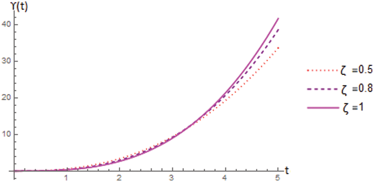
Figure 1: For ϒ(t) = t the graph in Fig. 1 shows the increasing behaviour with 0 + ≤ t ≤ 5
3 The Generalized Weighted Laplace Transform
In the following section, we use the weighted Laplace transformation to the new fractional operators. Firstly, we present the following definition which is a modified form of the Definition 1.5.
Definition 3.1. Suppose that the
holds for all values of u.
Proposition 3.1.
Proof. By the Definition 3.1, we have
Substitute
the proof is done.
Theorem 3.1. Let the function
where
Proof. By the Definitions 2.1, 1.6 and Proposition 3.1, we have
This completes the proof.
Theorem 3.2. The generalized weighted Laplace transform of the novel derivative is
Proof. By the Definition 2.2, Theorem 1.2 and Theorem 3.1, we get
The proof is completed.
4 Fractional Free Electron Laser Equation with Solution
In this section, we investigate the fractional generalization FEL by using the introduced fractional integral given in (2) and the fractional derivative presented in (3). The series form solution is obtained by employing the weighted generalized Laplace transform introduced by Jarad et al. [20].
Theorem 4.1. The solution of the cauchy problem
where
Proof. Applying generalized weighted Laplace transform on (9) and using Theorems 3.1 and 3.2, we get
The above equation implies that
Taking
By using the inverse Laplace transform, we obtain
the result is completed.
Remark 4.1. If we set
The following is the cauchy problem based on Theorem 4.1.
Example 4.1. The solution of the cauchy problem
where
subject to the condition
with
Solution 4.1. For the function given by (12) subjected to the condition presented in (13) the Eq. (11) becomes
Consider
Using (16) in (15), we obtain (14).
5 Fractional Kinetic Differ-Integral Equation with Solution
In the last decade, fractional calculus has opened up new vistas of research and brought a revolution in the study of fractional PDE’s and ODE’s [36–38]. Fractional kinetic equation has been successfully used to predict physical phenomena such as diffusion in permeable media, reactions and unwinding forms in complicated framework. The fractional form of the kinetic equation has gained attention due to the its relationship with the CTRW-theory [39]. This section is dedicated to investigating a new weighted fractional kinetic equations to explain the continuity of the motion of the material and the fundamental equations of natural sciences. The series solution of this new fractional kinetic equation by applying weighted generalized fractional laplace is also part of this section. The fractional kinetic equation is
subject to
where
Theorem 5.1. The solution of (17) with initial condition (18) is
Proof. By applying the modified weighted Laplace transform on both side of (17), we get
Using Theorems 3.1 and 3.2, we get
Taking
By applying the inverse Laplace transform, we get
Next, we include an example in the field of engineering using our defined operators.
Example 5.1. Consider a famous growth model given by
subject to the condition
where
Solution 5.1. By choosing
The graph of the function
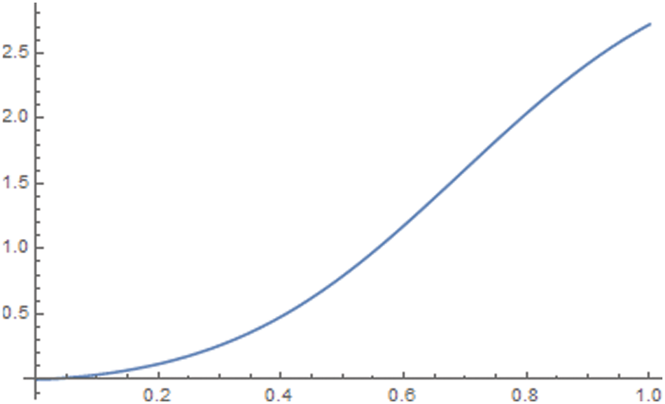
Figure 2: For 0 < α < 1, the graph in Fig. 2 indicates the increasing and convergent behaviour of the infinite series
In this paper, the weighted generalized fractional integral and derivative operators of Riemann-type are investigated. We discuss some properties of the fractional operators in certain spaces. Specifically, the semi-group and inverse properties are proved for the introduced operators. The modified weighted Laplace transform of novel operators is also examined which is compatible with the introduced operators. It is worth mentioning that many established operators unify some operators that exist in literature. Finally, the solutions of the weighted generalized fractional free electron laser and kinetic equations are obtained by utilizing the skillful technique of the weighted Laplace transform, which has been applied in many mathematical and physical problems. Furthermore, a Cauchy problem and a growth model for a specific choice of parameters involved are designed and sketched in their graphs to check the validity.
Acknowledgement: The authors T. Abdeljawad and K. Shah would like to thank Prince Sultan University for supporting through TAS research lab.
Funding Statement: The authors are thankful to Prince Sultan University for paying the article processing charges.
Conflicts of Interest: The authors declare that they have no conflicts of interest to report regarding the present study.
Reference
1. Hilfer, R. (2000). Applications of fractional calculus in physics. Singapore: World Scientific Publishing Co. Pte., Ltd. [Google Scholar]
2. Debnath, L. (2003). Recent applications of fractional calculus to science and engineering. International Journal of Mathematics and Mathematical Sciences, 54, 3413–3442. DOI 10.1155/S0161171203301486. [Google Scholar] [CrossRef]
3. Kilbas, A., Srivastava, H. M., Trujillo, J. J. (2006). Theory and application of fractional differential equations. North Holland: Elsevier. [Google Scholar]
4. Magin, R. L. (2006). Fractional calculus in bioengineering. USA: Begell House Publishers. [Google Scholar]
5. Podlubny, I. (1999). Fractional differential equations, mathematics in science and engineering. New York: Academic Press. [Google Scholar]
6. Samko, S. G., Kilbas, A. A., Marichev, O. I. (1993). Fractional integrals and derivatives: Theory and applications. Yverdon: Gordon and Breach. [Google Scholar]
7. Onal, M., Esen, A. (2020). A Crank-nicolson approximation for the time fractional burgers equation. Applied Mathematics and Nonlinear Sciences, 5(2), 177–184. DOI 10.2478/amns.2020.2.00023. [Google Scholar] [CrossRef]
8. Lozi, R., Abdelouahab, M. S., Chen, G. (2020). Mixed-mode oscillations based on complex canard explosion in a fractional-order FitzHugh-Nagumo model. Applied Mathematics and Nonlinear Sciences, 5(2), 239–256. DOI 10.2478/amns.2020.2.00047. [Google Scholar] [CrossRef]
9. Akdemir, A. O., Deniz, E., Yüksel, E. (2021). On some integral inequalities via conformable fractional integrals. Applied Mathematics and Nonlinear Sciences, 6(1), 489–498. DOI 10.2478/amns.2020.2.00071. [Google Scholar] [CrossRef]
10. Touchent, K. A., Hammouch, Z., Mekkaoui, T. (2020). A modified invariant subspace method for solving partial differential equations with non-singular kernel fractional derivatives. Applied Mathematics and Nonlinear Sciences, 5(2), 35–48. DOI 10.2478/amns.2020.2.00012. [Google Scholar] [CrossRef]
11. Kabra, S., Nagar, H., Nisar, K. S., Suthar, D. L. (2020). The marichev-saigo-maeda fractional calculus operators pertaining to the generalized K-struve function. Applied Mathematics and Nonlinear Sciences, 5(2), 593–602. [Google Scholar]
12. Koca, I., Yaprakdal, P. (2020). A new approach for nuclear family model with fractional order Caputo derivative. Applied Mathematics and Nonlinear Sciences, 5(1), 393–404. [Google Scholar]
13. Akgül, A. (2018). A novel method for a fractional derivative with non-local and non-singular kernel. Chaos, Solitons and Fractals, 114, 478–482. [Google Scholar]
14. Atangana, A., Baleanu, D. (2016). New fractional derivatives with non-local and non-singular kernel, theory and application to heat transfer model. Thermal Science, 20, 763–769. [Google Scholar]
15. Caputo, M., Fabrizio, M. (2015). A new definition of fractional derivative without singular kernel. Progress in Fractional Differentiation and Applications, 1(2), 73–85. [Google Scholar]
16. Modanli, M., Akgül, A. (2018). Numerical solution of fractional telegraph differential equations by theta-method. The European Physical Journal Special Topics, 226(16), 3693–3703. [Google Scholar]
17. Ghori, M. B., Naik, P. A., Zu, J., Eskandari, Z., Naik, M. (2022). Global dynamics and bifurcation analysis of a fractional-order SEIR epidemic model with saturation incidence rate. Mathematical Methods in the Applied Sciences, 45(4), 3665–3688. [Google Scholar]
18. Ahmad, B., Alghamdi, B., Agarwal, R. P., Alsaedi, A. (2022). Riemann-Liouville fractional integro-differential equations with fractional nonlocal multi-point boundary conditions. Fractals, 30(1), 2240002. [Google Scholar]
19. Henderson, J., Luca, R., Tudorache, A. (2022). On a system of Riemann-Liouville fractional boundary value problems with
20. Jarad, F., Abdeljawad, T., Shah, K. (2020). On the weighted fractional operators of a function with respect to another function. Fractals, 28(6), 2040011. [Google Scholar]
21. Agarwal, O. (2012). Some generalized fractional calculus operators and their applications in integral equations. Fractional Calculus and Applied Analysis, 15(4), 700–711. [Google Scholar]
22. Almeida, R. (2017). A Caputo fractional derivative of a function with respect to another function. Communications in Nonlinear Science and Numerical Simulation, 44, 460–481. [Google Scholar]
23. Jarad, F., Abdeljawad, T. (2020). Generalized fractional derivatives and laplace transform. Discrete and Continuous Dynamical Systems Series S, 13(3), 709–722. [Google Scholar]
24. Kiryakova, V. (2008). A brief story about the operators of generalized fractional calculus. Fractional Calculus and Applied Analysis, 11(2), 201–218. [Google Scholar]
25. Osler, T. (1970). Fractional derivatives of a composite function. SIAM Journal on Mathematical Analysis, 1(2), 288–293. [Google Scholar]
26. Al-Refai, M., Jarrah, A. M. (2019). Fundamental results on weighted Caputo-Fabrizio fractional derivative. Chaos, Solitons & Fractals, 126, 7–11. [Google Scholar]
27. Owolabi, K. M. (2018). Mathematical analysis and numerical simulation of chaotic noninteger order differential systems with Riemann-Liouville derivative. Numerical Methods for Partial differential Equations, 34(1), 274–295. [Google Scholar]
28. Diaz, R., Pariguan, E. (2007). On hypergeometric functions and pochhammer k-symbol. Divulgaciones Matematicas, 15(2), 179–192. [Google Scholar]
29. Samraiz, M., Umer, M., Kashuri, A., Abdeljawad, T., Iqbal, S. (2021). On weighted (k, s)-Riemann-Liouville fractional operators and solution of fractional kinetic equation. Fractal and Fractional, 5(3), 1–18. [Google Scholar]
30. Mubeen, S., Habibullah, G. M. (2012). k-fractional integrals and application. International Journal of Contemporary Mathematical Sciences, 7(2), 89–94. [Google Scholar]
31. Farid, G., Habibullah, G. M. (2015). An extension of hadamard fractional integral. International Journal of Mathematical Analysis, 9(9), 471–482. DOI 10.12988/ijma.2015.5118. [Google Scholar] [CrossRef]
32. Azam, M. K., Farid, G., Rehman, M. A. (2017). Study of generalized type k-fractional derivatives. Advances in Difference Equations, 2017, 1–12. DOI 10.1186/s13662-017-1311-2. [Google Scholar] [CrossRef]
33. Romero, L. G., Luque, L. L., Dorrego, G. A., Cerutti, R. A. (2013). On the k-Riemann-Liouville fractional derivative. International Journal of Contemporary Mathematical Sciences, 8(1), 41–51. DOI 10.12988/ijcms.2013.13004. [Google Scholar] [CrossRef]
34. Katugampola, U. N. (2014). A new approach to generalized fractional derivatives. Bulletin of Mathematical Analysis and Applications, 6(4), 1–15. [Google Scholar]
35. Colson, W. B. (1976). Theory of a free electron laser. Physics Letters A, 59(3), 187–190. DOI 10.1016/0375-9601(76)90561-2. [Google Scholar] [CrossRef]
36. Lü, Q., Zuazuayz, E. (2016). On the lack of controllability of fractional in time ODE and PDE. Mathematics of Control, Signals, and Systems, 28, 1–21. [Google Scholar]
37. Chen, J., Tepljakov, A., Petlenkov, E., Chen, Y. Q. (2020). State and output feedback boundary control of time fractional PDE–fractional ODE cascades with space-dependent diffusivity. IET Control Theory & Applications, 14(20), 3589–3600. DOI 10.1049/iet-cta.2019.1015. [Google Scholar] [CrossRef]
38. Lei, L., Liu, J. G. (2018). A generalized definition of caputo derivatives and its application to fractional ODEs. SIAM Journal on Mathematical Analysis, 50, 2867–2900. DOI 10.1137/17M1160318. [Google Scholar] [CrossRef]
39. Hilfer, R., Anton, L. (1995). Fractional master equations and fractal time random walks. Physical Review E, 51(2), 848–851. DOI 10.1103/PhysRevE.51.R848. [Google Scholar] [CrossRef]
Cite This Article
 Copyright © 2023 The Author(s). Published by Tech Science Press.
This work is licensed under a Creative Commons Attribution 4.0 International License , which permits unrestricted use, distribution, and reproduction in any medium, provided the original work is properly cited.
 Downloads
 Citation Tools