
 Submit a Paper
 Propose a Special lssue
 Open Access
ARTICLE

A Geometrically Exact Triangular Shell Element Based on Reproducing Kernel DMS-Splines
1 School of Aerospace Engineering, Beijing Institute of Technology, Beijing, 100081, China
2 China Academy of Launch Vehicle Technology, Beijing, 100076, China
* Corresponding Author: Hanjiang Chang. Email:
(This article belongs to the Special Issue: Integration of Geometric Modeling and Numerical Simulation)
Computer Modeling in Engineering & Sciences 2023, 136(1), 825-860. https://doi.org/10.32604/cmes.2023.022774
Received 25 March 2022; Accepted 19 September 2022; Issue published 05 January 2023
 View Full Text
 Download PDF
Abstract
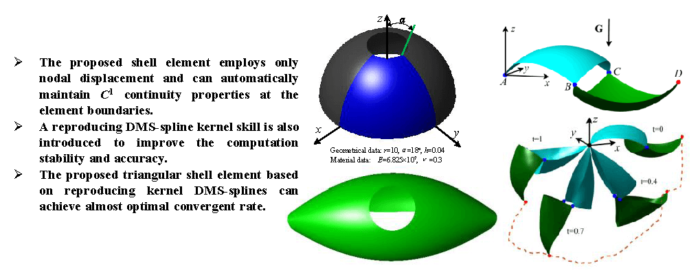
To model a multibody system composed of shell components, a geometrically exact Kirchhoff-Love triangular shell element is proposed. The middle surface of the shell element is described by using the DMS-splines, which can exactly represent arbitrary topology piecewise polynomial triangular surfaces. The proposed shell element employs only nodal displacement and can automatically maintain C1 continuity properties at the element boundaries. A reproducing DMS-spline kernel skill is also introduced to improve computation stability and accuracy. The proposed triangular shell element based on reproducing kernel DMS-splines can achieve an almost optimal convergent rate. Finally, the proposed shell element is validated via three static problems of shells and the dynamic simulation of a flexible multibody system undergoing both overall motions and large deformations.Graphic Abstract
Keywords
The nonlinear finite shell formulation has been successfully used to study numerous problems of shell structures over the past few decades [1]. According to the classic theory of shells [2], there are mainly two kinds of shells. That is, the thick shells with a ratio of edge length to thickness less than 20 and the thin shells with such a ratio larger than 20. In general, the thick shell is described by using the Reissner-Mindlin theory with the transverse shear deformations taken into account, while the thin shell is modeled by using the Kirchhoff-Love theory without the transverse shear deformations along the thickness direction. For many shell structures in practice, such as an accurate telescope assembled by different shell patches, the high-order continuity among shell patches is required. However, it is difficult to develop a Kirchhoff-Love element with C1 continuity by using the standard shape functions of Lagrange polynomials.
To reach a globally smooth and geometrically exact discretization, Hughes et al. [3] proposed the concept of the Isogeometric Analysis (IGA) in 2005. This technique has been considered as a benchmark method in the field of computational mechanics. The IGA based tensor-product B-splines/NURBS applications [4] can be found in many fields, such as structural mechanics [5–14], fluid mechanics [15–19], and contact mechanics [20–27]. In the field of multibody system dynamics, Shabana et al. [28] and Mikkola et al. [29] pointed out that the cubic B-spline curves and surfaces can be converted to the absolute nodal coordinate formulation (ANCF) for slender beam element and thin shell element without any geometric distortion. Sanborn et al. [30,31], and Lan et al. [32,33] proposed a thin beam element of rational ANCF (RANCF) with the same original CAD geometry of the cubic NURBS curves. In addition, Nada [34] proposed a plate element based on the B-spline surface in the case of large deformations. Yamashita et al. [35] comparatively studied the convergence of finite element solutions of B-spline and ANCF beam element. They found that the B-spline element and the ANCF element with same orders and continuities will lead to identical results. Based on the Integration of Computer Aided Design and Analysis (I-CAD-A) technique, three new ANCF triangular shell elements represented by Bézier triangles are proposed by Chang et al. [36], which enriches the family of ANCF elements. Again, Goyal et al. [37] and Maurin et al. [38] respectively extended the Isogeometric Euler-Bernoulli beam element and Kirchhoff-Love quadrilateral shell element to model flexible multibody dynamics. Phung-Van et al. [39] used the IGA plate to study the functionally graded piezoelectric material under thermo-electro-mechanical loads. Compared with the plate elements with traditional Lagrange interpolation, their results indicated that the accuracy and reliability for the geometrically nonlinear responses of the plate can be obtained.
Over the past few years, many IGA based Kirchhoff-Love rectangular shell elements [2,12,14,37, 40,41] have been proposed. However, the application of these elements is limited because a single B-spline/NURBS patch can only represent the surfaces of rectangular topological type. In general, an arbitrary topological shell surface can be described by using the network of B-spline/NURBS patches. Nevertheless, it is difficult to enforce a certain degree of continuity between the adjacent shell patches [4]. The major drawback of the B-spline/NURBS is that the gaps at intersections of shell surfaces can not be avoided. In addition, the complicated parameterization of the arbitrary topological computation domain is a time-consuming task [42]. Besides, one B-spline/NURBS patch utilizes a tensor product structure, which makes the representation of the detailed local features inefficient. In order to achieve the local refinement, the T-splines have been further incorporated into the IGA [43–46]. Till now, it is still a challenge to model the complicated geometry with an arbitrary topology by T-splines, because it is not easy to obtain the linear dependent T-splines [47]. In order to achieve the continuity and the local refinement in the arbitrary topological computation domain, Hughes et al. [3] pointed out that it is an opportunity for research in IGA to develop the isogeometric analysis with triangle or tetrahedron elements. Rational Bézier triangles are used for domain triangulation of complex geometries by Liu et al. [48,49], which increase the flexibility in discretization.
In fact, in the field of computer graphics and computer aided design, the DMS-splines [50] (also named triangular B-splines) can be used to describe a broad class of objects with arbitrary and non-rectangular topology. The DMS-spline surfaces are able to provide an elegant and unified representation scheme for all the piecewise continuous polynomial surfaces over a planar parametric domain [51]. The other feature that makes DMS-splines attractive for surface description is their low degree. For example, a C1 continuous surface can be constructed by using the quadratic DMS-splines, which have the parametric degree 2 in total. However, if the standard quadratic tensor–product surfaces such as B-spline/NURBS surfaces are used, the parametric degree in total will be 4. Franssen et al. [52] proposed an efficient scheme to evaluate the DMS-splines in modeling the complex smooth surfaces. Qin et al. [53,54] presented the DMS-splines and rational DMS-splines to model the free form surface with non-rectangular topology. This method is based on the dynamic behavior of the model results in response to the applied forces and constraints. Pfeifle et al. [55] proposed a method to fit the DMS-spline surface by using the scattered points data, and obtained the smooth surfaces by combining the least squares method and bending energy minimization method. Furthermore, Mihalík used the DMS-splines to model the human head surface [56,57], and proposed an effective algorithm for generating the knot-net.
In general, the global continuity and local refinement surfaces can be modeled with the DMS-splines, while the DMS-splines do not perform well in computer aided engineering without adjustment [58] as a direct surface approximation based on the DMS-splines is sensitive to the placement of knots. When the knots are far from or very close to the vertices of the triangles in the parametric domain, the DMS-splines may numerically deviate from the partition of unity property, and the summation of their derivatives may not be close to zero [59]. Thus, the direct use of the DMS-splines as the interpolation functions may lead to considerable errors in the approximation of the DMS-spline surfaces in the computational domain. In order to address this problem, according to the reproducing kernel element method, Sunilkumar et al. [59] proposed the reproducing kernel DMS-splines (RKDMS) to remove the unexpected errors and instability of the DMS-splines. Sunilkumar et al. [59] and Jia et al. [58] obtained the optimal convergence rate in in solving 2D linear solid problems and the partial differential equations (PDEs) based on the RKDMS, respectively. Sunilkumar et al. [60] further proposed the smooth DMS-spline finite element method and used the method to solve nearly incompressible nonlinear elasto-static problems. Sunilkumar et al. [61] also studied the wrinkled and slack of nonlinear 3D elastic membranes based on the smooth DMS–splines finite element method, and obtained satisfactory results compared with the results of the laboratory experiments. Nevertheless, it is still an open problem to establish the thin shell elements based on the RKDMS.
The objective of this study is to propose a geometrically exact Kirchhoff-Love triangle shell element based on the RKDMS. The rest of the paper is organized as follows. In Section 2, a brief review of DMS-splines is given, and the RKDMS evaluation schemes are systematically presented. Then, the geometrically exact Kirchhoff-Love triangle shell element is derived in Section 3. To compute the generalized internal force vector and the Jacobian matrix of the shell element, the derivative evaluation schemes of RKDMS are also deducted in this section. The solution strategies of the dynamic equations are presented in Section 4. Finally, in Section 5, the results of several static problems of shells are provided to validate the proposed shell element, and the dynamics of a flexible multibody system is simulated. In Section 6, the main conclusions of the study are drawn, and the future studies on this subject are outlined.
2 Reproducing Kernel DMS-Splines
The DMS-splines were originally proposed by Dahmen et al. [50] in 1992. The theoretical foundation of DMS-splines is based on the simplex splines of approximation theory [52]. The simplex splines are the multivariate generalization of the univariate B-splines. In order to represent the DMS-spline surface with triangular topology, the basic concept of the simplex splines are firstly revisited.
2.1 Description of the Simplex Splines
A simplex spline of degree n is a smooth, piecewise polynomial function defined by a set of n + Ndim + 1 points described by a position vector t
where p(ξ, η) is an arbitrary point in the planar parametric domain Ω described by the orthogonal cartesian coordinate system O-ξ-η, as shown in Fig. 1, and W = (w0, w1, w2)
where t0 = (t0ξ, t0η), t1 = (t1ξ, t1η), and t2 = (t2ξ, t2η) are three knots in the knot-set V. λi(p|W), (i = 0, 1, 2) are the barycentric coordinates of the point p(ξ, η) respected to the triangle W with three vertexes w0, w1, w2. As illustrated in Fig. 1, the three barycentric coordinates λi(p|W) can be defined as
where S denotes the area of the triangle
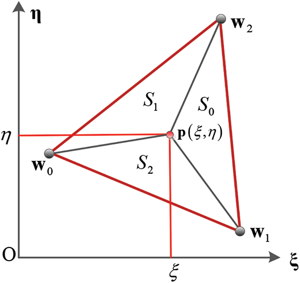
Figure 1: Schematic view of the barycentric coordinates
In Eq. (1), [V) stands for a half open convex hull, the readers can refer to the work by Farin [62] to know how to construct a half-open convex hull of a triangle. Fig. 2 shows some simplex splines. Fig. 2a gives a simplex spline of degree zero with three knots t0 = (0.2, 0.2), t1 = (0.7, 0.2), t2 = (0.5, 0.6), Fig. 2b presents a linear simplex spline with four knots t0 = (0.2, 0.2), t1 = (0.6, 0.7), t2 = (0.3, 0.6), t3 = (0.7, 0.1), and Fig. 2c illustrates a quadratic simplex spline with five knots t0 = (0.2, 0.2), t1 = (0.6, 0.1), t2 = (0.9, 0.3), t3 = (0.7, 0.7) and t4 = (0.4, 0.6). From Fig. 2, it can be found that the constant simplex spline is discontinuous at its domain boundary, the linear spline is C0 continuity and the quadratic simplex spline is C1 continuity. Therefore, in order to represent the mid-surface of Kirchhoff shell element with C1 continuity, we focus on the quadratic simplex spline. According to Eq. (1), the quadratic simplex spline can be calculated by the linear combination of three linear simplex splines. Similarly, the single linear simplex spline can be calculated by a similar recurrent procedure with the combination of three constant simplex splines. Fig. 3 gives a schematic view of the quadratic simplex spline M(p|{t0, t1, t2, t3, t4}) calculation process.
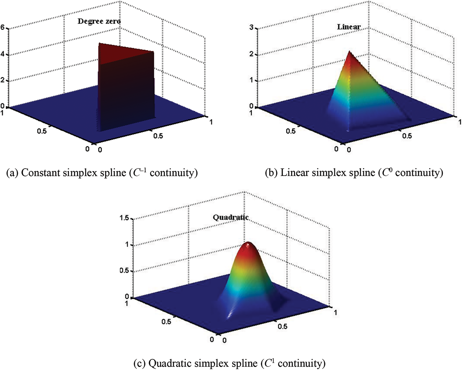
Figure 2: Simplex spline examples
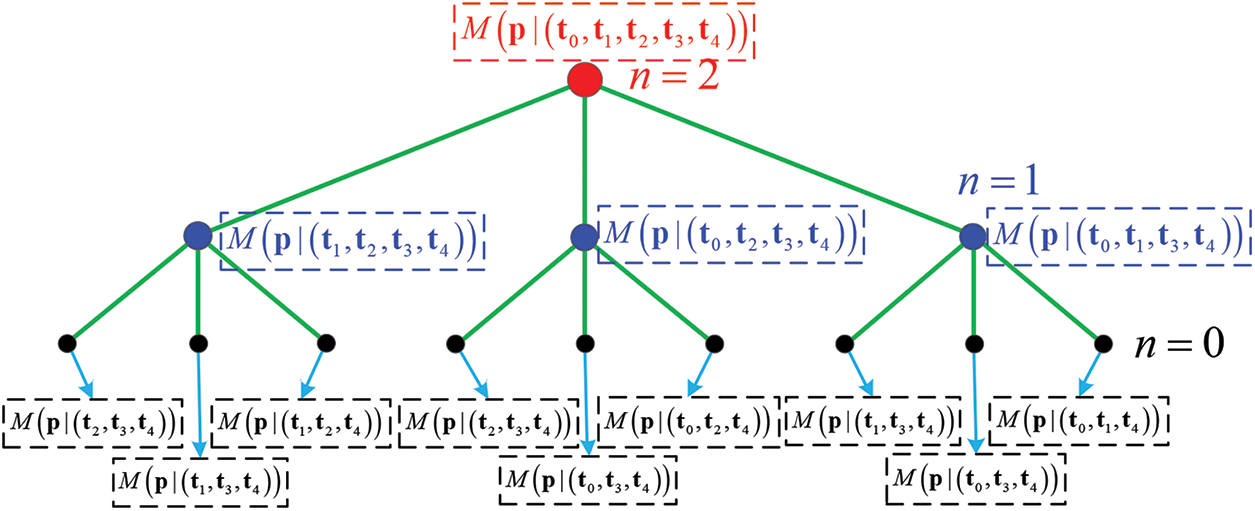
Figure 3: Tree structure of the entire calculation the quadratic simplex spline
2.2 Description of the DMS-Splines
The DMS-splines, which in fact are the weighted sum of the simplex splines, are the functions that possess the features of the global smoothness and the local supporting [51]. Different from the concept of the knot-set defined in the Section 2.1, the knot-net is used to define the DMS-splines.
Let K = {t00,…, t0n, t10,…, t1n, t20,…, t2n} be a knot-net associated with the triangle Δ = [t0, t1, t2] = [t00, t10, t20], where n is the polynomial degree of DMS-splines. ti0 (i = 0, 1, 2) are called the root knots. For each root knot, there are n extra knots connected to the corresponding root knot. The set of the n + 1 knots Ci = {ti0, … , tin} is called the knot-cloud associated with the root knot ti = ti0. For the definition of the DMS-spline, several knot-sets
where
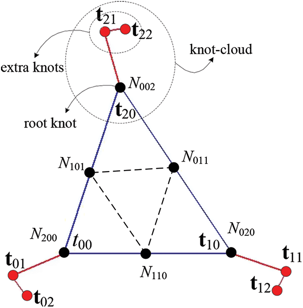
Figure 4: Distribution of DMS-splines for quadratic case with knots
A DMS-spline surface is generally composed of several surface patches with separate triangles on the parametric domain, as illustrated in Fig. 5. The position of an arbitrary point on the DMS-spline surface can be expressed by
where m is the total number of the DMS-splines, and ci is the control point of the DMS-spline surface defined in the global coordinate system X-Y-Z.
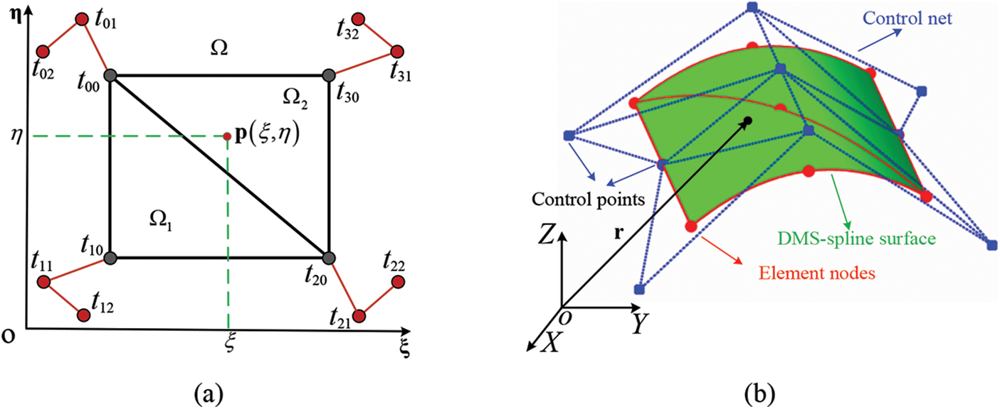
Figure 5: (a) Triangulation domain composed of two triangles. (b) Graph of the quadratic DMS-spline surface
From Fig. 5, it can be found that the non-zero contributions of the particular surface patch are not only in the areas of the corresponding triangle but also in the surrounding triangles, because the DMS-splines have a larger definitional domain compared with the triangle domain composed of the three root knots ti0 (i = 0, 1, 2). This feature is the main difference from the classical methods of construction smooth triangular surfaces [62]. If the non-zero contributions of the particular surface patch are only in the areas of corresponding triangle, the DMS-splines will degenerate into Bézier triangles. The interference of the DMS-spline surface patches ensures a global smoothness of the whole surface without any additional limitations on the control points. The triangulation shown in Fig. 5a is composed of two triangles with one adjoining side and two shared vertices. For the quadratic DMS-spline surface, there are 12 knots and 9 control points. A quadratic DMS-spline surface for the triangulation and a control net are shown in Fig. 5b. From Fig. 5b, it can be seen that the control points are not located on the DMS-spline surface.
From the above analysis, it can be found that the location of the knots in the parametric domain play an important role in determining the DMS-splines. A major restriction on the position of the knot-cloud is that three knots can not be collinear [57] for a smooth surface. This is a severe task to obtain the knot-cloud over the parametric domain. In this study, the algorithm for generating the knot-net proposed by Mihalík [57] is adopted. This method considers the distance between the main knot and the extra knot as the only variable. The distance is defined as approximately 8% of the triangle shortest side in the parametric domain, and this choice is found to work well for most problems [59,60]. The knot–cloud configurations based on this knot-net generation algorithm with internal and external boundaries are shown in Fig. 6.
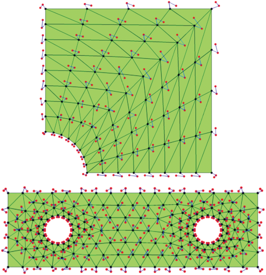
Figure 6: Knots for constructing the quadratic DMS-spline surfaces
2.3 Reproducing Kernel DMS-Splines
The DMS-splines have been proposed more than two decades. However, till now there is no robust rule or criteria to show how to construct the analysis-suitable DMS-splines. The challenge is due to the flexibilities of the DMS-splines. The performance of the DMS-splines is influenced by the uniformity of triangulation and the placement of knot clouds. From Eq. (4), although the quadratic DMS-splines are C1 continuous, the DMS-splines may numerically deviate from the partition of unity property [3] and the summation of their derivatives may not be close to zero [59]. These drawbacks could account for many unexpected errors occurring in the numerical quadrature for the stiffness matrix and generalized internal force vector. In order to overcome this problem, the reproducing kernel approximation technique is adopted to improve the numerical stability and accuracy of the DMS-splines in this study. This idea is motivated by the reproducing kernel particle method [63–66], which is one of the most popular mesh-free methods. It improves the shape functions through multiplying the original shape functions by some correction terms. In IGA, this technique has been successfully applied to solve the mechanics problem with the tensor product NURBS in non-rectangular topology [67].
According to the work by Sunilkumar et al. [59], the improved approximation for the DMS-splines can be expressed as
where Φi(ξ, η) are the improved shape functions containing the correction parts. qi are the generalized coordinates located on the DMS-spline surface, as illustrated in Fig. 5b. The improved shape functions can be written as
where bT(ξ, η)H(ξ–ξi, η–ηi) is the correction term for the shape functions. H(ξ–ξi, η–ηi) is a set of polynomial basis
Considering that the improved shape functions should be satisfied the partition of unity and higher order polynomial reproducing properties, the coefficient vector b(ξ, η) in Eq. (7) can be determined by following conditions [58]
It is easy to prove that the first two equations of Eq. (9) can be a unified expression with the last equation of Eq. (9). For example, for the last equation of Eq. (9), if α = β = 0,
where H(0) = [1, 0, …, 0]T is a constant (n + 1) × (n + 1)/2 by 1 vector, and the moment matrix D is a square matrix of order (n + 1) × (n + 1)/2, which can be expressed by: [59]
Thus, the coefficient vector b can be obtained rapidly by solving the small-scale linear Eq. (10). Finally, substituting the coefficient vector b into Eq. (7), the improved shape functions Φi(ξ, η) yield the following implicit form:
It is should be noted that as the coefficient vector b depends on the location of the parameter (ξ, η), the detailed expressions of the improved shape functions are varied in the parameter domain. The evaluation of coefficient vector b for the quadrature points can be accomplished in the preprocessing stage of the finite element analysis, which will not decay the computational efficiency.
3 Kirchhoff-Love Shell Element Based on the RKDMS
3.1 Kinematic Description and Equilibrium Equation
According to the Kirchhoff-Love shell theory, the shell transverse shear deformation is neglected and the straight lines normal to the mid-surface will remain normal to the mid-surface after deformation. As shown in Fig. 7, πz describes an arbitrary layer parallel to the mid-surface π of the thin shell. In the initial reference configuration, the global position of an arbitrary point
where the subscript ‘0’ indicates the initial state, ξ1 and ξ2 can be regarded as the convective curvilinear coordinates of the shell, and ζ denotes the distance between the mid-surface π and the surface πz, with −h/2 ≤ ζ ≤ h/2, h is the shell thickness. r0 indicates the position vector of the corresponding point P0(ξ1, ξ2) on the mid-surface π, which can be described by using the reproducing kernel DMS-spline surface. n0 is the unit normal vector of the mid-surface π at point P0(ξ1, ξ2). For further deformation analysis, a local curved surface coordinate frame (g0z)1-(g0z)2-(g0z)3 and an element local orthogonal coordinate frame (e0z)1-(e0z)2-(e0z)3 are defined at the point
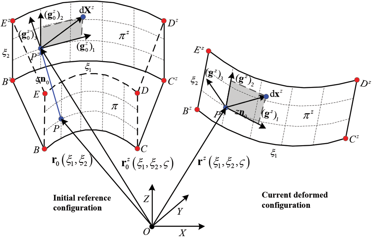
Figure 7: General motion of a thin shell element
According to the continuum mechanics [62], the matrix of deformation gradient F can be expressed as
where dX0 denotes the infinitesimal arc segment defined in the initial reference configuration, and dx0 indicates the deformed arc segment defined in the current configuration. The deformation gradient F can be decomposed with an orthogonal matrix R and a nonsingular symmetric matrix U, written as
where the right stretch tensor U can be extracted via decomposition from the deformation gradient F by separating the rigid-body rotation R, and they can be expressed as
where R denotes the transformation matrix of the two local Cartesian coordinate frames (ez)1-(ez)2-(ez)3 and (e0z)1-(e0z)2-(e0z)3, and the matrix T0 denotes the transformation matrix from (e0z)1-(e0z)2-(e0z)3 to (g0z)1-(g0z)2-(g0z)3, which can be expressed as
Similarly, in the current configuration the matrix T can be expressed as
According to continuum mechanics and the orthogonality relation between vectors (e0z)1 and (e0z)2, the Green–Lagrange strain of the layer πz of the shell element can be written as
where
Finally, the Green-Lagrange strain tensor ε can be recast as
where εmem represents the membrane strain of the shell element, and εbend denotes the bending strain of the shell element and can be further cast as
where
Using a St. Venant-Kirchhoff material model in order to describe an isotropic and linear elastic material, the second Piola-Kirchhoff stress tensor σs can be written in Voigt notation
where E is the Young’s modulus and ν is the Poisson’s ratio. ε11, ε12, and ε22 are the three components of the Green-Lagrange strain tensor ε.
Substituting Eqs. (20) and (21) into (23) and integrating the Eq. (23) through the thickness direction ζ, −h/2 ≤ ζ ≤ h/2, the stress resultant with the membrane strains σn can be defined
and the bending strains σm can be written as
where
The internal virtual work is defined by
For solving the nonlinear equation system Eq. (26), the Newton–Raphson method is used,
where Δq is the infinitesimal increment of the element generalized coordinates q.
Based on Eq. (28), the first derivative of the virtual work is the residual force vector Fr
where Fext is the external load vector and Fint is the vector of generalized internal forces,
The second derivatives of the virtual work yield the Jacobians J, which can be written as
The Jacobian matrix Jint is obtained by deriving the above term for the internal virtual work with the generalized coordinates
where the first two terms represent the material part of stiffness matrix and the latter two the geometrical part of stiffness matrix. When calculating the generalized internal force vector Fint and the Jacobian matrix Jint, the first and second derivative of the RKDMS should be involved, which will be discussed in detail in the following subsection. Besides, the numerical quadrature is applied to calculate the Jacobian matrix Jint and the generalized internal force vector Fint over each triangle parametric domain A, while the supports of the shape functions are not aligned with the integration domain [70]. In order to minimize the numerical quadrature error, the triangle parametric domain is subdivided into 9 sub-triangles. In our implementation we choose 3 Gauss quadrature points in each sub-triangle for the quadratic RKDMS.
3.2 Evaluation the Derivative of the RKDMS
In order to calculate the generalized internal force vector and the Jacobian matrix deduced in the previous subsection, the first and second derivative of the reproducing kernel DMS-splines with respect to the parameter coordinates are required. According to Eq. (1), the first derivative of the DMS-splines can be calculated as follows [58]:
where
Substituting Eq. (34) into Eq. (33), the derivative of the DMS-splines can be calculated, and the second derivative of the DMS-splines also can be calculated in the same way. The quadratic DMS-splines and their derivatives to ξ are illustrated in Figs. 8 and 9, respectively.
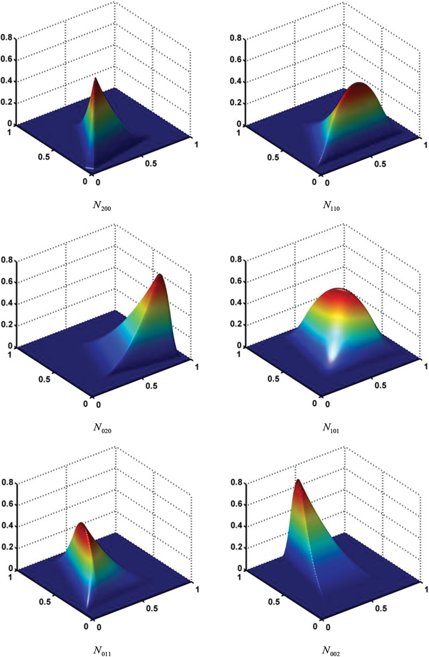
Figure 8: Schematic view of quadratic DMS-splines
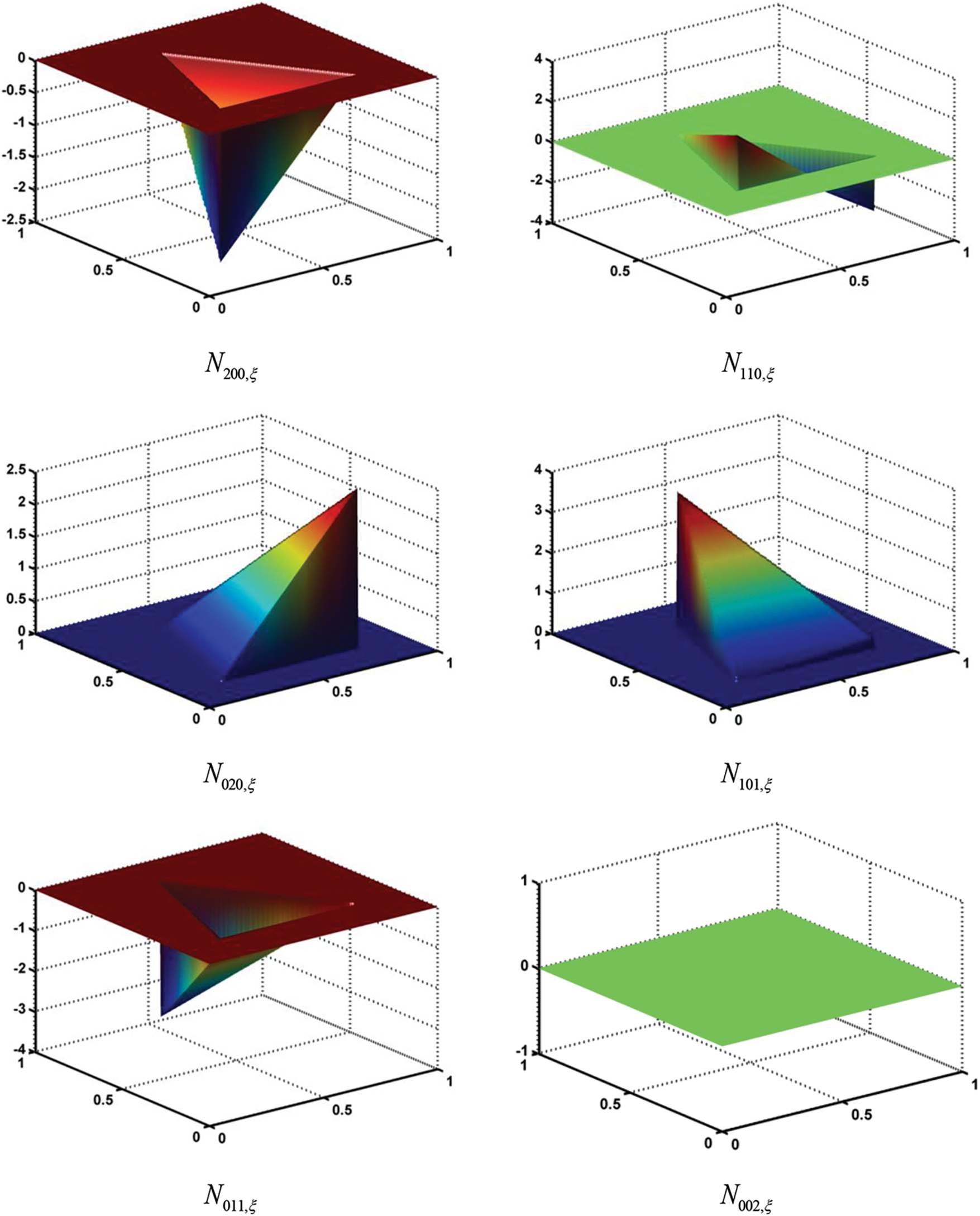
Figure 9: Schematic view of quadratic DMS-spline derivatives
From above analysis, based on the Eq. (7), the derivatives of the reproducing kernel DMS-splines Φi(ξ, η) could be calculated by
where
Obviously,
Substituting Eq. (37) into Eq. (35), the derivative of the reproducing kernel DMS-splines Φi(ξ, η) can be obtained. The reproducing kernel DMS-splines and their derivatives have been constructed through Eqs. (7) and (35), respectively. The quadratic RKDMS and their derivatives to ξ are illustrated in Figs. 10 and 11, respectively. In the Kirchhoff-Love shell theory, the second order derivatives of the reproducing kernel DMS-splines with respect to the parameter coordinates need to be considered to calculate the bending strain. Furthermore, the second derivatives can be calculated with the similar method.
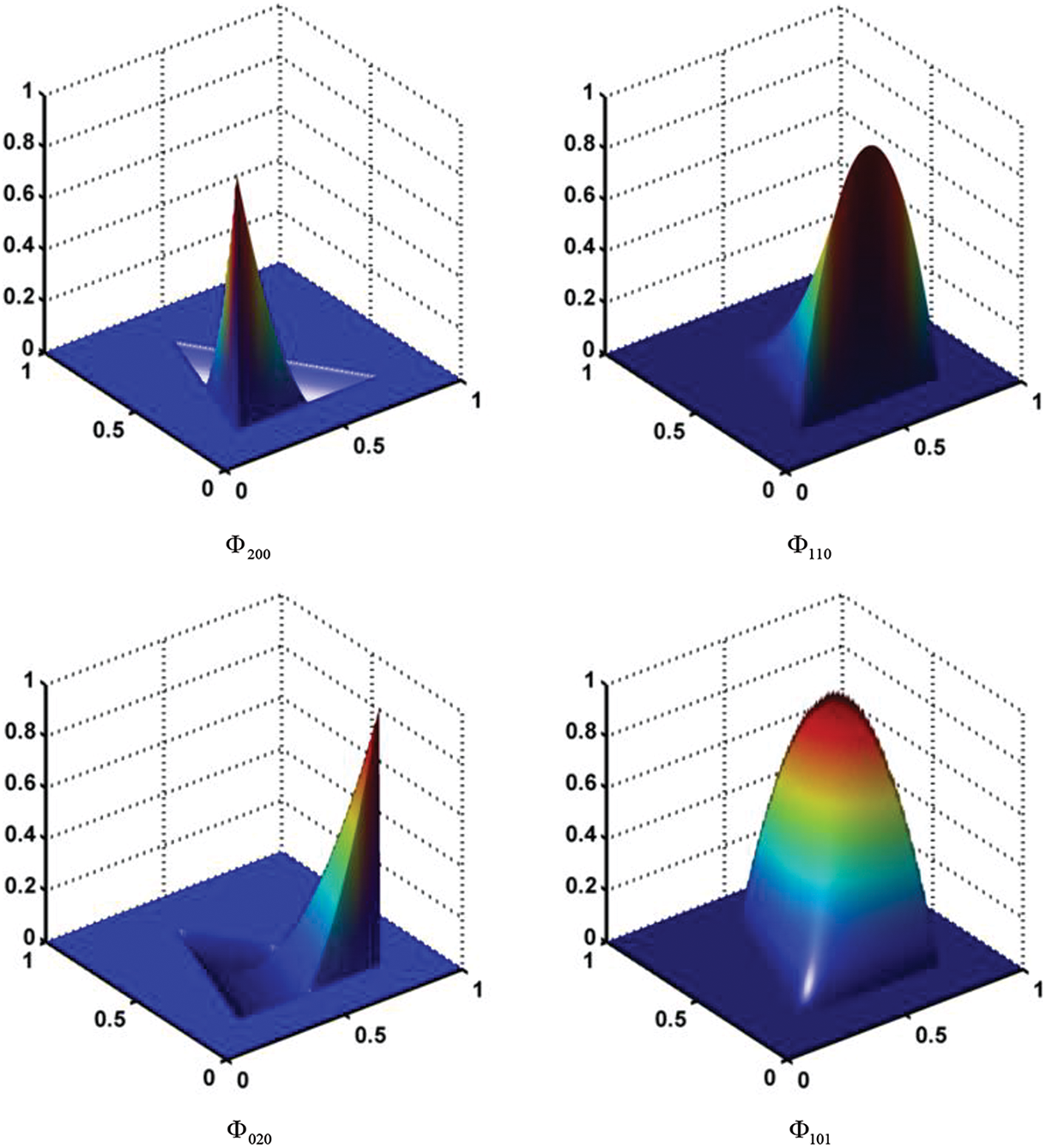
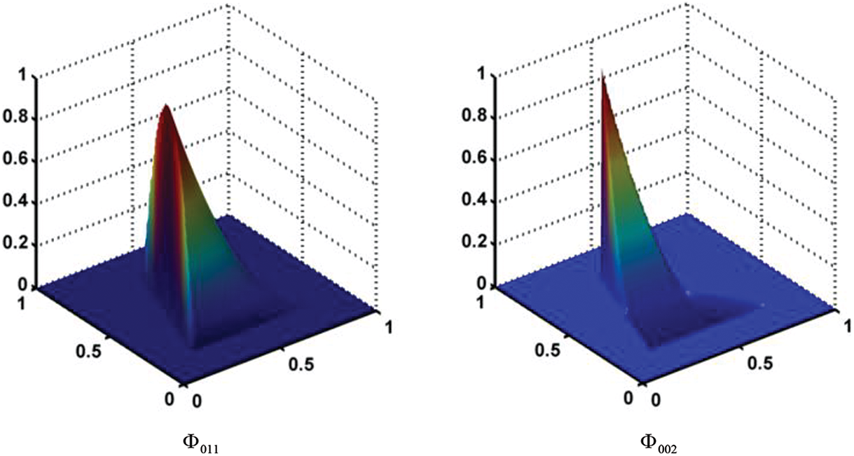
Figure 10: Schematic view of a quadratic RKDMS
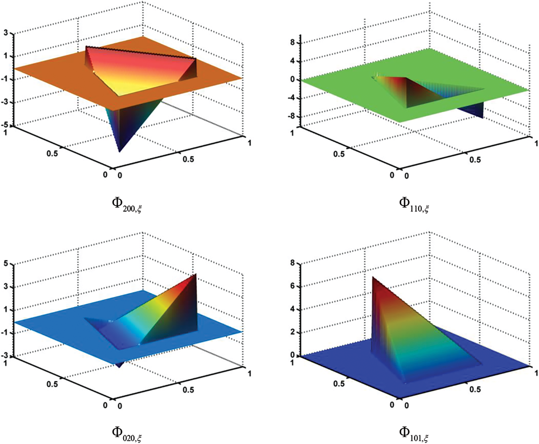
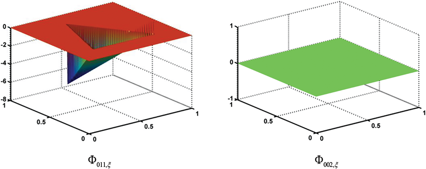
Figure 11: Schematic view of the quadratic RKDMS derivatives
4 Computation Solution Strategy for Flexible Shell Multibody Systems Dynamics
According to the assembly procedure of finite elements, the dynamic equation of a constrained flexible multibody system can be expressed as a set of differential algebraic equations as follows [71]:
where M is the mass matrix of the system, Fint is the elastic force vector, φ represents the vector containing the system constraints and φq is the corresponding Jacobian with respect to the generalized coordinates q, λ is the vector of Lagrange multipliers, and Fext is the vector of external generalized forces, which can be obtained by using the principle of virtual work from Eqs. (30) and (32).
In the present study, the generalized-alpha implicit algorithm proposed by Chung et al. [72] is used to solve Eq. (38). This algorithm enables one to reach an optimal combination of accuracy at the low-frequency range and numerical damping at the high-frequency range. Some studies [73,74] indicated that the generalized-alpha algorithm is identical to ‘the three parameters optimal schemes’ originally proposed by Shao et al. [75,76]. These two identical algorithms have exhibited good applicability to even tougher problems solved by Liu et al. [77–79] and Tian et al. [80] by in studying the dynamics of a flexible multibody system with clearance joints. Readers can also gain an insight into the efficient parallel computation strategy in the work by Liu et al. [79–81].
5 Case Studies and Discussions
In this section, the proposed shell element is firstly validated via three static problems of shells. Then, the validated shell element is used to study the dynamics of a flexible multibody system of shells undergoing both overall motions and large deformations.
5.1 Infinite Plate with Circular Hole under Constant in–Plane Tension
The first case study focuses on a classic linear elasto-static problem of an infinite plate with a stress-free circular hole under uniform tension, as shown in Fig. 12. The structural symmetry of the problem enables one to study a quarter of the plate only. The geometric and material parameters used are: the radius of the hole is R = 0.5, the edge length of the finite quarter plate is L = 2, the Young’s modulus is E = 105 and the Poisson’s ratio is ν = 0.3.
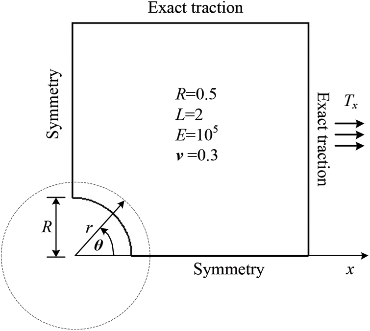
Figure 12: Infinite elastic plate with a circular hole: problem domain, boundary conditions, and material parameters
Under the Neumann boundary condition [3], the problem yields an exact solution as follows:
where Tx = 10 is the magnitude of the applied stress for the infinite plate, (r, θ) are the polar coordinates. The traction boundary conditions are imposed on the right (x = 2) and top (y = 2) edges, and the symmetry boundary conditions are imposed on the left (x = 0) and bottom (y = 0) edges, respectively.
A comparison is made for the convergence rate of the L2 norm of the stress error obtained by using the quadratic element, the Bézier triangle element [36], the DMS-splines element and the RKDMS element. Fig. 13 shows the five models with different mesh sizes. Fig. 14 shows the L2 norm of the stress errors corresponding to the meshed models shown in Fig. 13. It is obvious that the quadratic RKDMS element has the best convergence rate compared with other elements. In Tables 1–3, h denotes the longest edge length of all the triangle elements and the DOFs stands for the degrees of freedom. It can be found that the results obtained by using the quadratic RKDMS element are much more accurate than those from other elements. As can be seen in Table 3, the convergence rate of the L2 norm of the stress error for the quadratic RKDMS element is 1.82, which is close to the optimal convergence rate. However, Tables 1 and 2 show that the convergence rates of the quadratic DMS and Bezier elements are not as good as that of the quadratic RKDMS element. All the comparison results show that the reproducing kernel technique of can significantly enhance the convergence rate of a shell element.
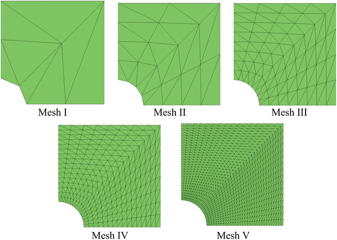
Figure 13: Infinite elastic plate with a circular hole: meshes discretization for the quadratic case employed in the error convergence study
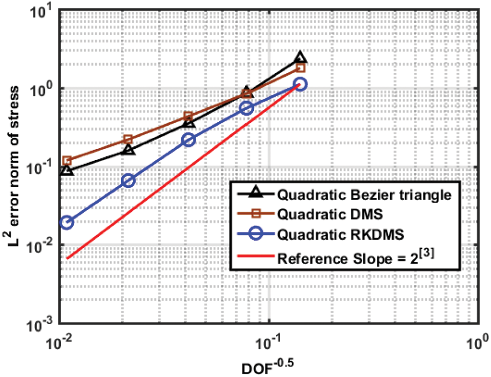
Figure 14: Convergence of the L2 norm of the stress error for quadratic Bézier triangle, quadratic DMS-splines and quadratic RKDMS with different mesh discretization
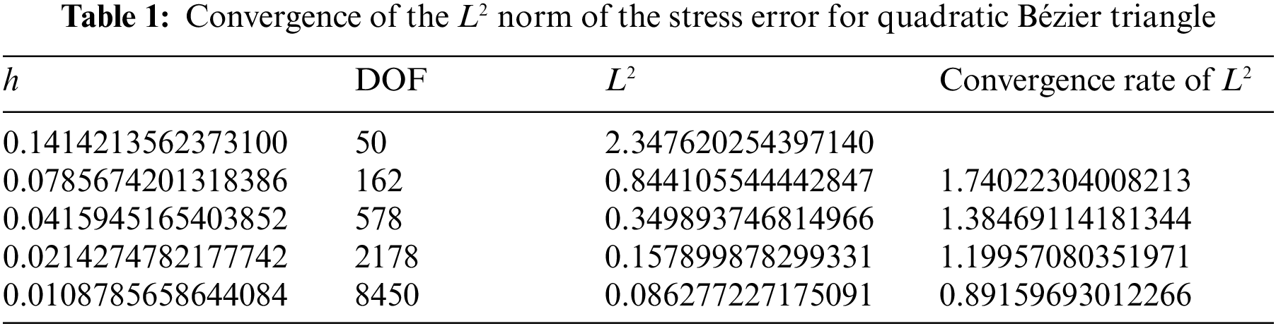
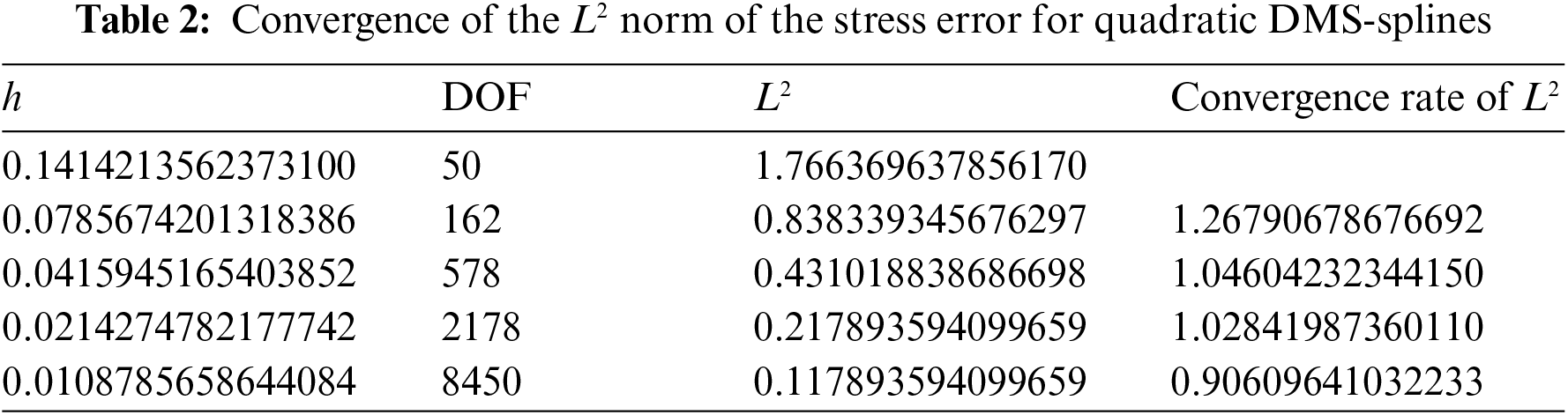
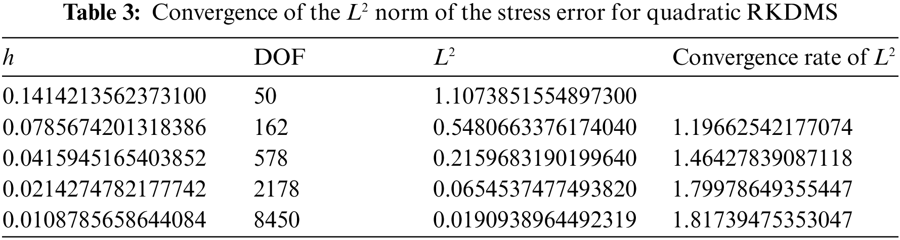
Fig. 15 presents the σxx contours for the mesh V discretized by three kinds of elements. The figure indicates that the stress contour obtained by using the RKDMS elements is smoother and more accurate than those from the Bézier element and DMS-splines element. In addition, the stress results achieved by using the RKDMS element are in a good agreement with the analytical solutions.
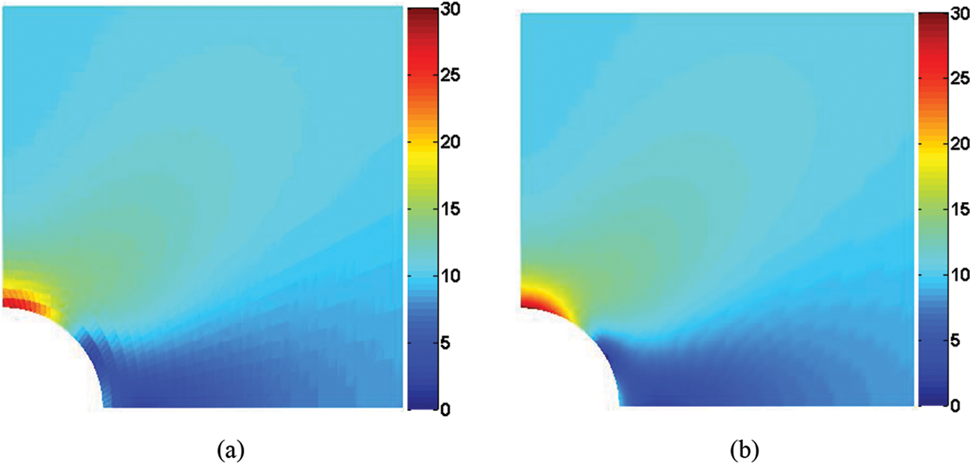
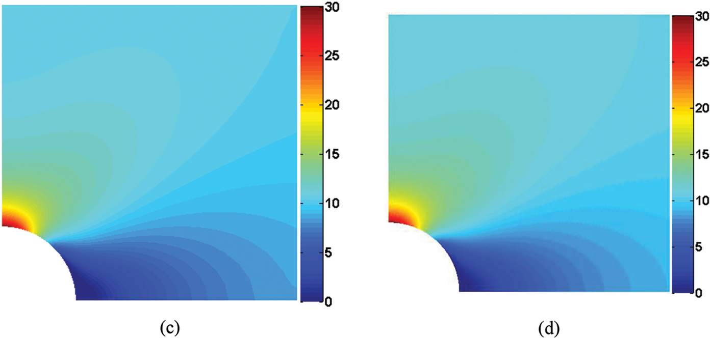
Figure 15: Contour plots of
5.2 Nonlinear Clamped Plate under a Uniformly Distributed Load
The second case study is a square plate subject to a uniformly distributed pressure, as illustrated in Fig. 16. This problem has been studied by Ubach et al. [82], Stolarski et al. [83] and Valdés et al. [84]. Now, the geometric and material parameters are taken as the same in those studies. That is, the length of the plate is L = 2a = 20, the thickness is h = 1, the Young’s modulus is E = 12 and the Poisson’s ratio is ν = 0. Similar to the first case study, only a quarter of the plate OMBN should be studied. The symmetric boundary conditions are imposed along two edges OM and ON, while the other two edges BM and BN are clamped.
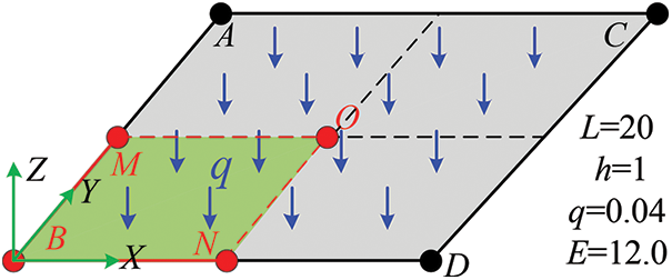
Figure 16: A nonlinear clamped plate under uniformly distributed load
Fig. 17 presents three structured mesh models (Mesh I: 50 elements with 121 nodes; Mesh II: 200 elements with 441 nodes; Mesh III: 800 elements with 1681 nodes) and one unstructured mesh model (Mesh IV: 813 elements with 1702 nodes) for the plate OMBN with quadratic RKDM elements. To study the influence of the load magnitude on the results, the transversal displacement w at the central point of the plate is normalized with respect to the thickness h, while the uniform distributed load q is normalized with respect to Dh/a4, with D = Eh3/12.
Figure 17: Different mesh models
Fig. 18 gives the ‘load-displacement’ curves of the mesh models. To make a comparison, the problem is also solved by using 1600 S4R elements in the commercial software ABAQUS. Fig. 18 indicates that the converged result is in a good agreement with those from ABAQUS. Besides, the results of the structured Mesh III well agree with those of the unstructured mesh IV. Fig. 18 also shows the importance of geometrically nonlinear effects on large displacements compared with the linear analysis. Fig. 19 gives the vertical displacement contours of the deformed models.
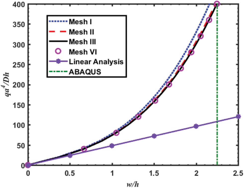
Figure 18: Load vs. center displacement of point O for the plate problem (The reference result with ABAQUS is 2.2507)
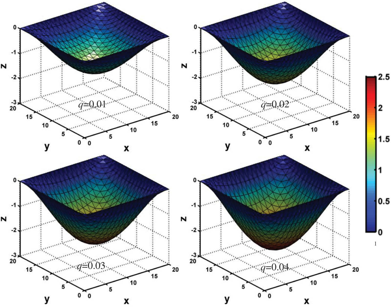
Figure 19: Vertical displacement contours and deformation configurations of models under different loads
5.3 Buckling Analysis of a Pinched Cylinder with Free Edges
This example is a popular benchmark problem in the field of finite element technology and provides a severe test for the RKDMS proposed in this paper. The same model has been studied by previous works [36,77]. As shown in the Fig. 20, a free cylindrical shell is subjected to two opposite concentrated force at the midpoint of the top and bottom surface. As suggested in previous literatures, the length of the cylindrical shell, L, is set to be 10.35, and the inner radius, R, and the thickness are 4.953 and 0.094, respectively. The force applied at the shell is 40. The elastic material properties is represented by the Young’s modulus E = 10.5 × 10⁶ and Poisson’s ratio v = 0.3125. As a consequence, the results provided by this paper are compared with those preformed in previous works and the results calculated by the commercial software ABAQUS.
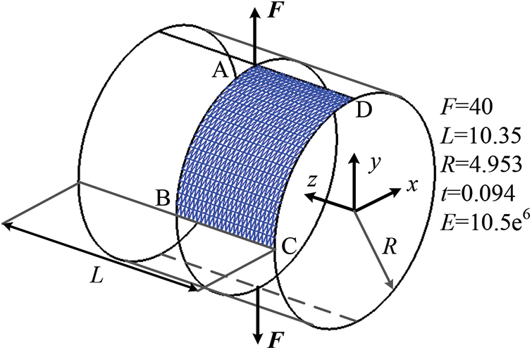
Figure 20: Buckling analysis of a pinched cylinder with free edges: Initial configuration and material parameters
By taking into account the symmetry considerations, only the one upper quarter of the structure is studied. The applied load for this problem is outward relative to the shell surface, and the ends of the cylinder are free. Three meshes with different number of elements are shown in Fig. 21, and the ‘load-displacement’ curves of the corresponding mesh are presented in Fig. 22, where
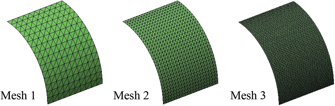
Figure 21: Thin cylindrical shell surface meshes: Meshes 1–3
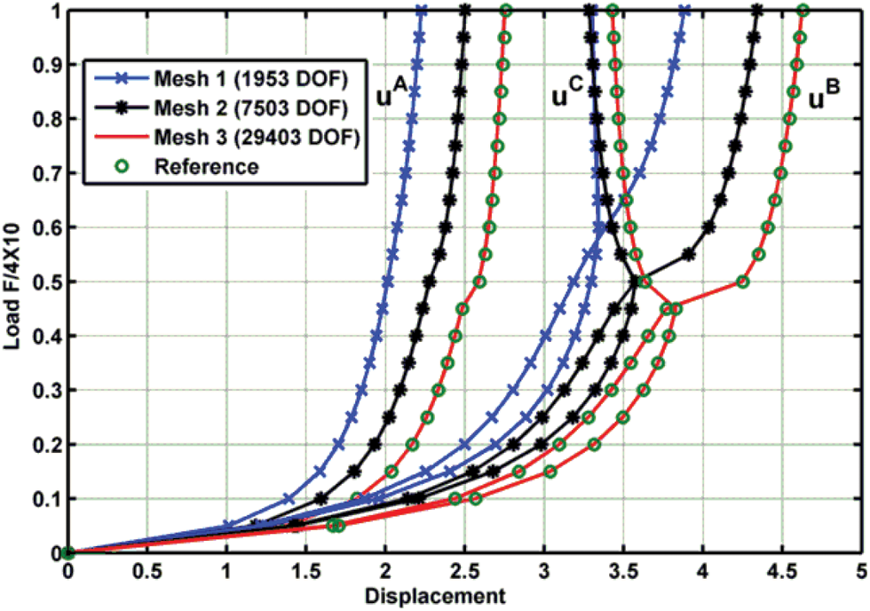
Figure 22: Magnitudes of displacements at nodes A, B and C
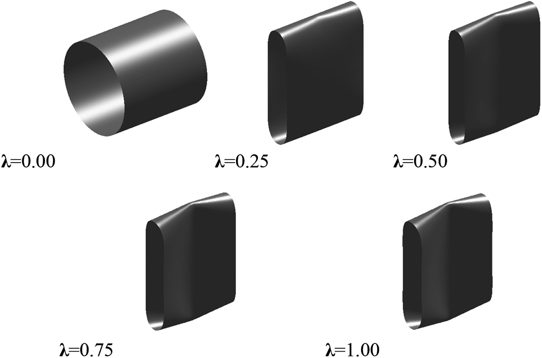
Figure 23: Deformed configurations of the cylinder under pulling forces with Mesh 3
The fourth case study focuses on two hemispherical shells. One has an 18° hole as shown in Fig. 24 and the other does not have any hole. The two hemispherical shells have been used to validate the shell elements in many works [85,86].
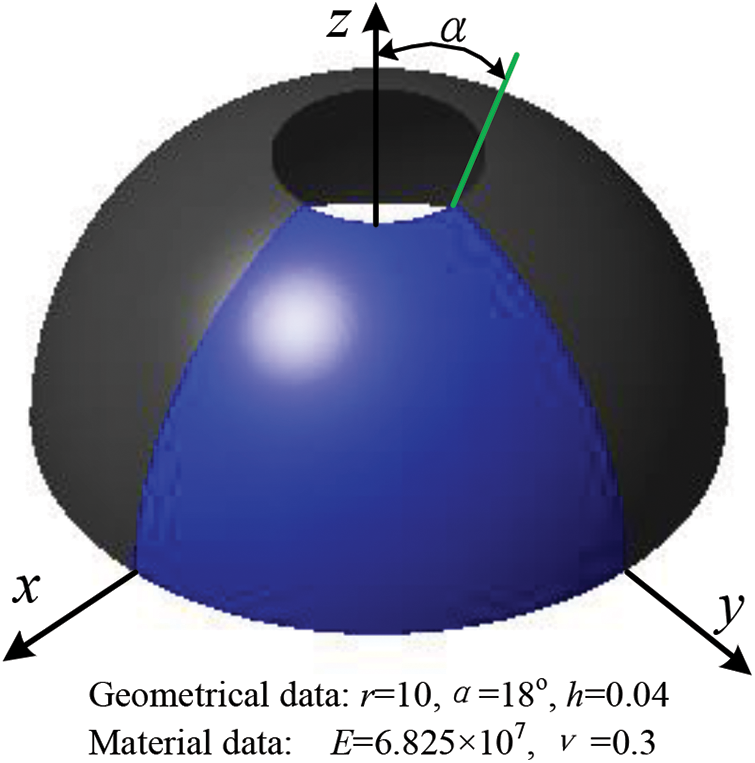
Figure 24: The problem statement of the hemispherical shell with 18° hole
For the hemispherical shell with an 18° hole at one side, the geometric and material parameters, as well as the load, are the same as those in previous literatures. That is, the radius r = 10, the thickness h = 0.04, the Young’s modulus E = 6.825 × 10⁷, and the Poisson’s ratio ν = 0.3. Only a quarter of the shell needs to be studied because of the structural symmetry. The initial geometry (Fig. 25b) is mapped from a plane rectangular reference configuration (Fig. 25a) with a mesh of 4 × 4 × 2 elements via the following spherical mapping
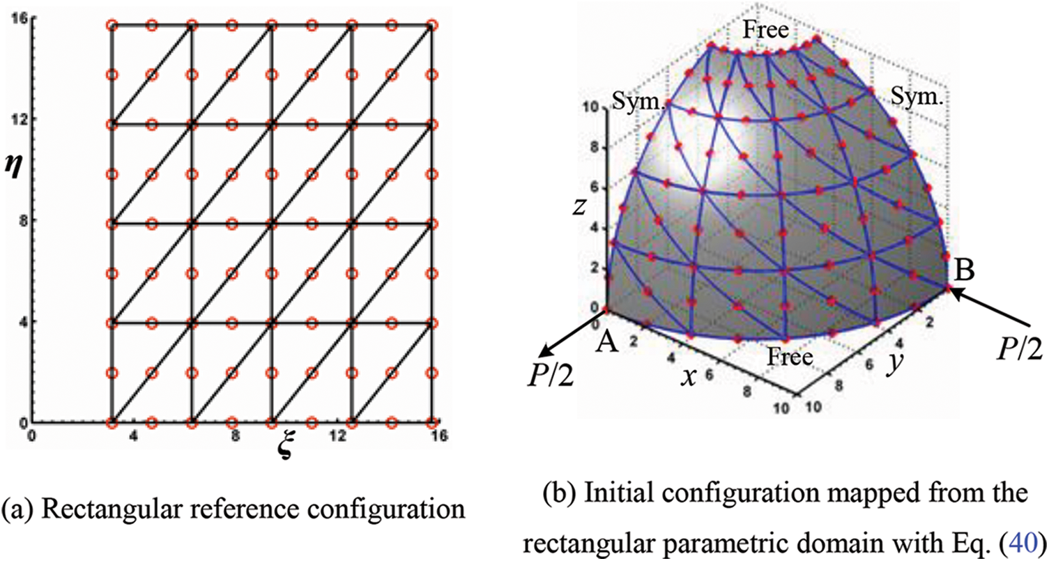
Figure 25: Hemispherical shell with 18o hole-reference and initial configurations
The displacements of point A and B under P = 400 are shown in Table 4, where the results well agree with those obtained by using the S4R shell element in software ABAQUS, and the results look better with an increase of the element number. Besides, the deformed shape of the whole shell for the final load step is depicted in Fig. 26, simultaneously the precision of the imposed symmetry conditions can be visually assessed.
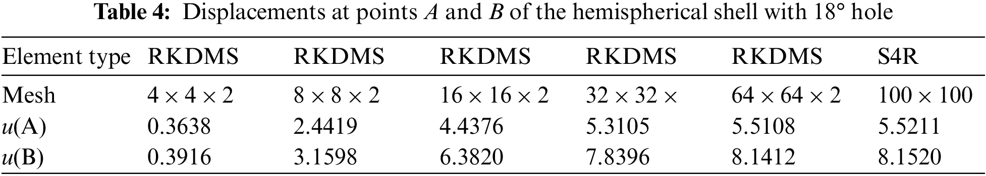

Figure 26: Deformed configuration of the hemispherical shell with 18° hole for the load P = 400
The hemispherical shell without any hole has the same geometric and material parameters as the hemispherical shell with a hole, but is a more challenging problem. To perform the dynamic simulation by using the proposed method, an initial discretization from Fig. 27a is replaced by the one from Fig. 25a. The spherical mapping in Eq. (40) is still applied to the discretization from Fig. 23a to build the initial configuration in Fig. 27b. The alternative triangular reference configuration from Fig. 27c can also be considered for the solution of the full hemispherical shell problem. The specific mapping in Eq. (41) is designed to build a complete sphere octant of the prescribed radius, see Fig. 27d. The symmetric boundary conditions are imposed along the horizontal and diagonal sides of the reference domain.
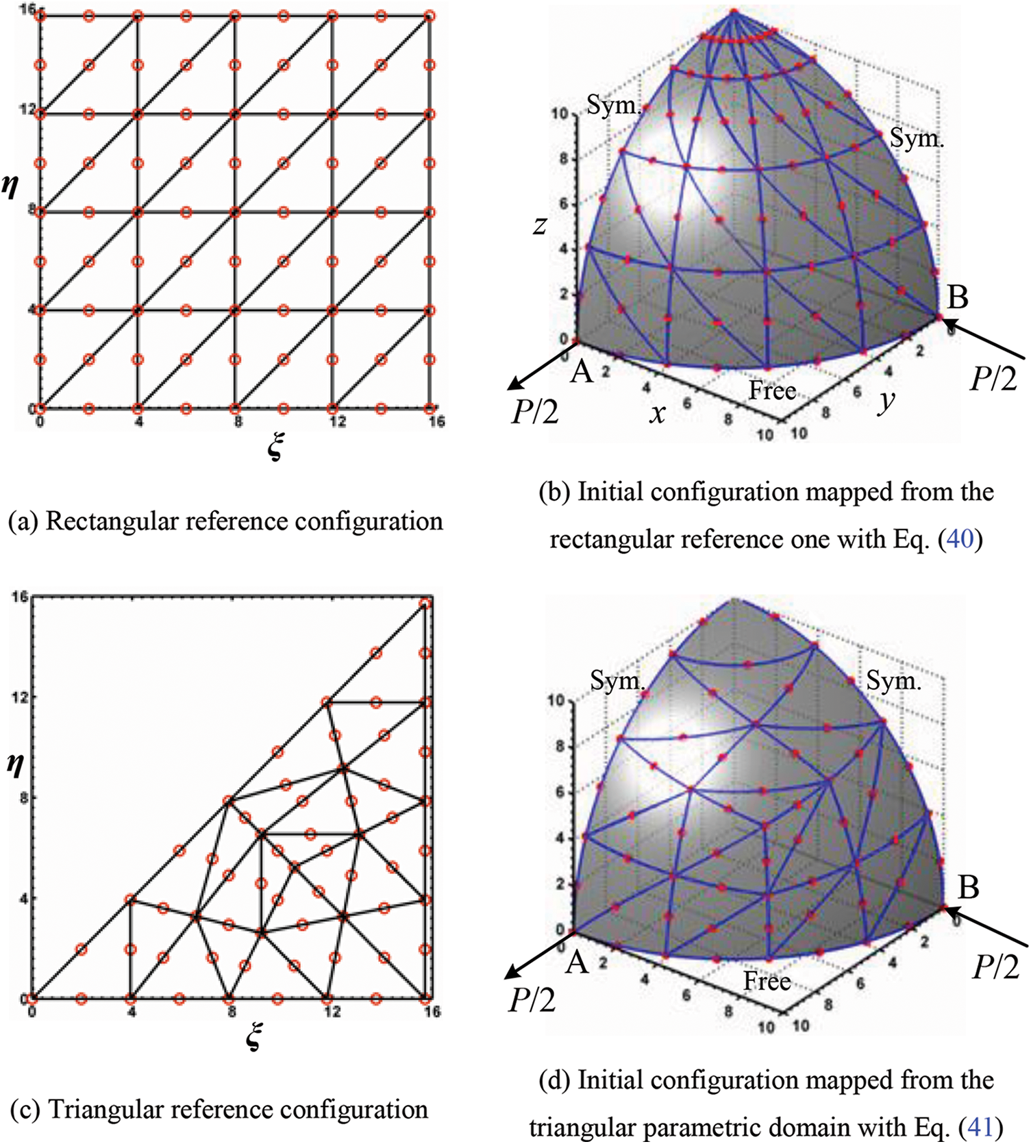
Figure 27: The hemispherical shell configurations
In order to perform a fair comparison of efficiency of these two reference configurations, the displacements of points A and B under P = 400 are shown in Tables 5 and 6, respectively. It is obvious that the triangular reference configuration provides better results than the rectangular one. The results based on the proposed formulation are in a good agreement with those simulated with dense S4R element in ABAQUS. Fig. 28 shows the deformed configuration of the hemispherical shell under the load P = 400.
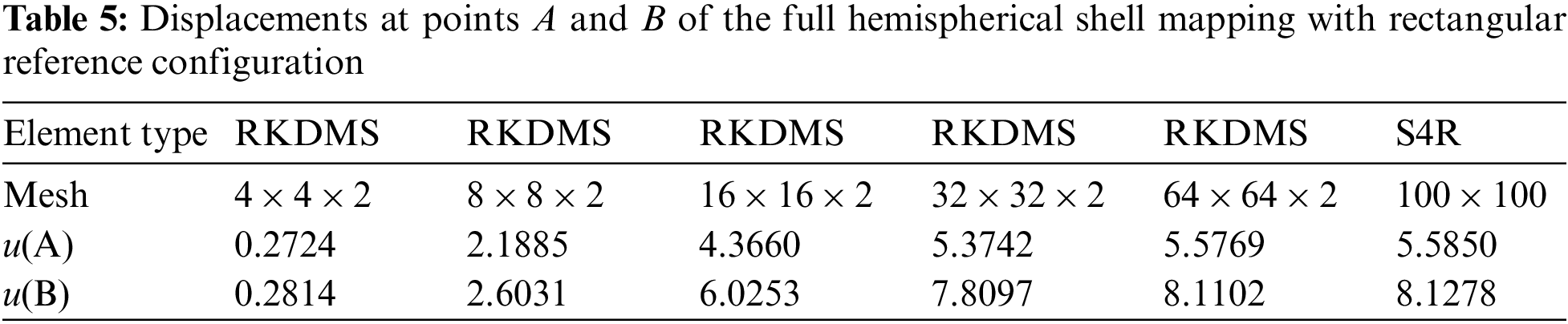
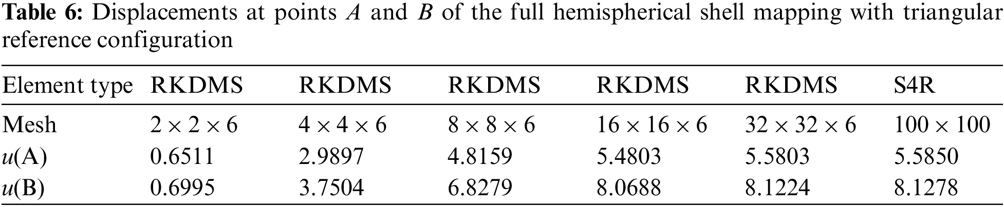
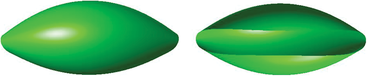
Figure 28: Deformed configuration of the full hemispherical shell for the finial load P = 400
5.5 Dynamics of a Double Pendulum Composed of Two Octant Spherical Shells
The final case study is to simulate the dynamics of a double pendulum composed of two identical octant spherical shells, as shown in Fig. 29. The initial geometry of an octant spherical shell is mapped from a plane triangular reference configuration with Eq. (41). The Young’s modulus of the material is 6.825 × 10⁷ Pa, and the material density is 7810 kg/m3, and the Poisson’s ratio is 0.3. The geometry properties are radius of 0.5 m and thickness of 0.01 m, and the gravitational acceleration is chosen as 9.81 m/s2. The four corner points A, B C and D are initially located on the horizontal plane x-y with the concave side upward for one shell and the concave side downward for the other shell. The corner point A is restrained to the ground via a spherical joint, which prevent the corner point A from any translation displacement, but does not limit any rotation. The two shells are connected with two spherical joints at points B and C, as shown in Fig. 29.
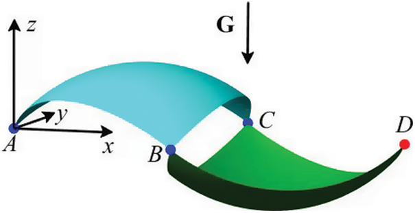
Figure 29: Initial configuration of the double pendulum
An objective of this case study is to check the influence of the number of the proposed thin shell elements on the system dynamics. As shown in Fig. 30, the difference of the system displacement at point D in z-direction becomes smaller and smaller with an increase of the number of finite elements. Fig. 30 indicates that the mesh of 8 × 8 × 12 shell elements is enough to give convergent results. To ensure the correctness of the simulation dynamics, it is helpful to check the total energy of the system, as shown in Fig. 31, with respect to time, where T, V and U are kinetic energy, deformation energy and potential energy of the system, respectively. As the double pendulum is a conservative system, the total energy should be a constant all the time. Fig. 31 presents the energy conservation holds true for the model, with a mesh of 8 × 8 × 12 shell elements. Fig. 32 shows the dynamic configuration of the system at four specific moments.
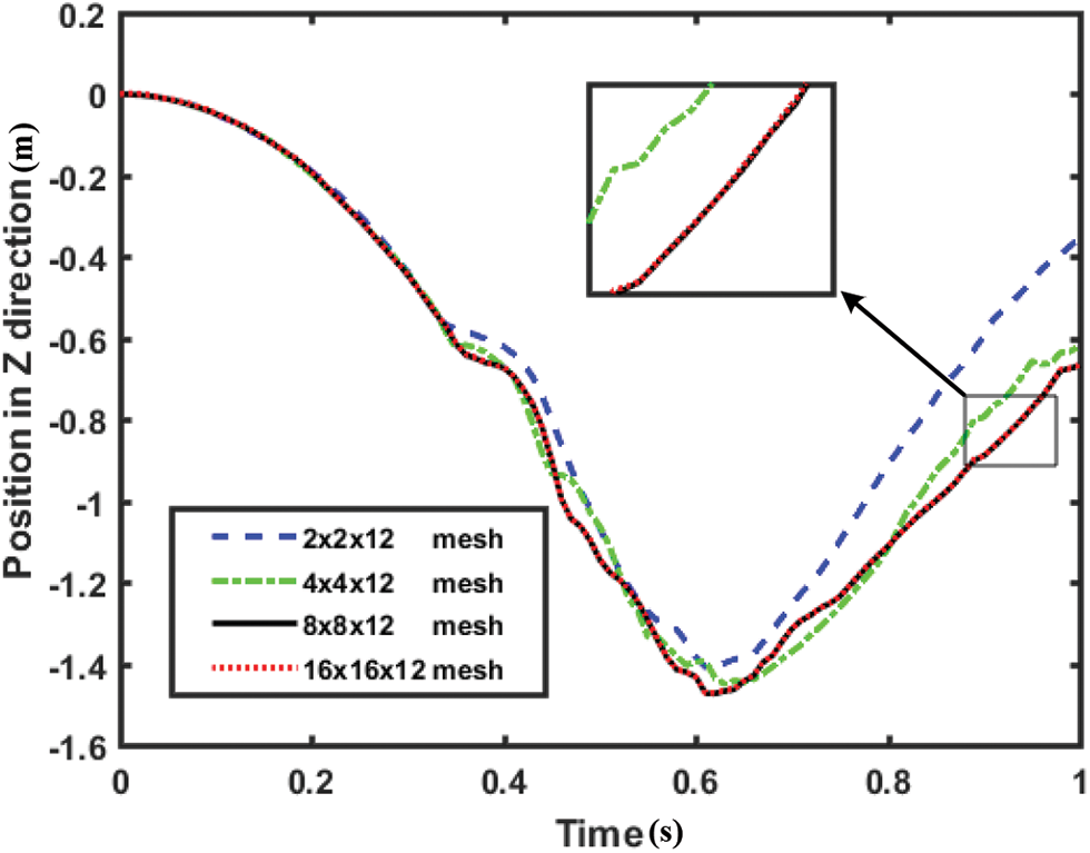
Figure 30: The motion of point D in z–direction of the double pendulum with different mesh densities
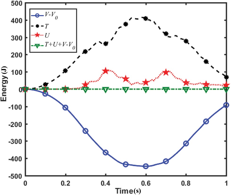
Figure 31: Energy balance of the free falling double pendulum
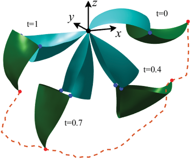
Figure 32: Dynamic deformed configurations of the double pendulum (8 × 8 × 12 mesh)
The paper presents how to establish a geometrically exact Kirchhoff-Love shell element via the reproducing kernel DMS-splines for the dynamics of multibody systems. The procedure is general and can be applied to thin shell systems with complex topology. The reproducing kernel DMS-splines surface has shown to be well-suited for modeling Kirchhoff–Love shell elements because it is easy to reach the C1 continuity. The number of degrees of freedom of the proposed shell elements is quite low compared with the traditional thin shell elements based on the standard shape functions of Lagrange, because each node of the shell element has only three translational degrees of freedom. In addition, the reproducing kernel approximation of the DMS-splines ensures the computation stability and accuracy of the proposed shell element, and improves the convergence rate of the proposed formulation. The paper demonstrates the efficacy of the proposed formulation via four static problems of shells, as well as the dynamic simulation of a flexible double pendulum composed of shells undergoing both overall motion and large deformation. As a part of future work, it is possible to extend the technique to more complicated systems based on tetrahedral meshes and the trivariate DMS-splines.
Funding Statement: This work was supported in part by the National Natural Science Foundations of China under Grants 11290151, 11672034 and 11902363.
Conflicts of Interest: The authors declare that they have no conflicts of interest to report regarding the present study.
References
1. Belytschko, T., Liu, W. K., Moran, B., Elkhodary, K. I. (2014). Nonlinear finite elements for continua and structures. 2nd edition. Chichester: John Wiley & Sons Ltd. [Google Scholar]
2. Kiendl, J., Bletzinger, K. U., Linhard, J., Wüchner, R. (2009). Isogeometric shell analysis with Kirchhoff–Love elements. Computer Methods in Applied Mechanics and Engineering, 198(49), 3902–3914. DOI 10.1016/j.cma.2009.08.013. [Google Scholar] [CrossRef]
3. Hughes, T. J. R., Cottrell, J. A., Bazilevs, Y. (2005). Isogeometric analysis: CAD, finite elements, NURBS, exact geometry and mesh refinement. Computer Methods in Applied Mechanics and Engineering, 194(39–41), 4135–4195. DOI 10.1016/j.cma.2004.10.008. [Google Scholar] [CrossRef]
4. Rogers, D. F. (2001). An introduction to NURBS: With historical perspective. San Diego, CA: Academic Press. [Google Scholar]
5. Weeger, O., Wever, U., Simeon, B. (2013). Isogeometric analysis of nonlinear Euler–Bernoulli beam vibrations. Nonlinear Dynamics, 72(4), 813–835. DOI 10.1007/s11071-013-0755-5. [Google Scholar] [CrossRef]
6. Sang, J. L., Park, K. S. (2013). Vibrations of Timoshenko beams with isogeometric approach. Applied Mathematical Modelling, 37(22), 9174–9190. DOI 10.1016/j.apm.2013.04.034. [Google Scholar] [CrossRef]
7. Adam, C., Bouabdallah, S., Zarroug, M., Maitournam, H. (2014). Improved numerical integration for locking treatment in isogeometric structural elements, Part I: Beams. Computer Methods in Applied Mechanics and Engineering, 279, 1–28. DOI 10.1016/j.cma.2014.06.023. [Google Scholar] [CrossRef]
8. Bauer, A. M., Breitenberger, M., Philipp, B., Wüchner, R., Bletzinger, K. U. (2016). Nonlinear isogeometric spatial Bernoulli beam. Computer Methods in Applied Mechanics and Engineering, 303, 101–127. DOI 10.1016/j.cma.2015.12.027. [Google Scholar] [CrossRef]
9. Ghafari, E., Rezaeepazhand, J. (2017). Isogeometric analysis of composite beams with arbitrary cross–section using dimensional reduction method. Computer Methods in Applied Mechanics and Engineering, 318, 594–618. DOI 10.1016/j.cma.2017.02.008. [Google Scholar] [CrossRef]
10. Benson, D. J., Bazilevs, Y., Hsu, M. C., Hughes, T. J. R. (2010). Isogeometric shell analysis: The Reissner–Mindlin shell. Computer Methods in Applied Mechanics and Engineering, 199(5), 276–289. DOI 10.1016/j.cma.2009.05.011. [Google Scholar] [CrossRef]
11. Kapoor, H., Kapania, R. K. (2012). Geometrically nonlinear NURBS isogeometric finite element analysis of laminated composite plates. Composite Structures, 94(12), 3434–3447. DOI 10.1016/j.compstruct.2012.04.028. [Google Scholar] [CrossRef]
12. Kiendl, J., Hsu, M. C., Wu, M. C. H., Reali, A. (2015). Isogeometric Kirchhoff–Love shell formulations for general hyperelastic materials. Computer Methods in Applied Mechanics and Engineering, 291, 280–303. DOI 10.1016/j.cma.2015.03.010. [Google Scholar] [CrossRef]
13. Dornisch, W., Müller, R., Klinkel, S. (2016). An efficient and robust rotational formulation for isogeometric Reissner–Mindlin shell elements. Computer Methods in Applied Mechanics and Engineering, 303, 1–34. DOI 10.1016/j.cma.2016.01.018. [Google Scholar] [CrossRef]
14. Goyal, A., Simeon, B. (2016). On penalty–free formulations for multipatch isogeometric Kirchhoff–Love shells. Mathematics and Computers in Simulation, 136, 78–103. DOI 10.1016/j.matcom.2016.12.001. [Google Scholar] [CrossRef]
15. Bazilevs, Y., Calo, V. M., Zhang, Y., Hughes, T. J. R. (2006). Isogeometric fluid–structure interaction analysis with applications to arterial blood flow. Computational Mechanics, 38(4–5), 310–322. DOI 10.1007/s00466-006-0084-3. [Google Scholar] [CrossRef]
16. Bazilevs, Y., Calo, V. M., Hughes, T. J. R., Zhang, Y. (2008). Isogeometric fluid–structure interaction: Theory, algorithms, and computations. Computational Mechanics, 43(1), 3–37. DOI 10.1007/s00466-008-0315-x. [Google Scholar] [CrossRef]
17. Nguyen, M. N., Bui, T. Q., Yu, T., Hirose, S. (2014). Isogeometric analysis for unsaturated flow problems. Computers and Geotechnics, 62, 257–267. DOI 10.1016/j.compgeo.2014.08.003. [Google Scholar] [CrossRef]
18. Kamensky, D., Hsu, M. C., Schillinger, D., Schillinger, D., Evans, J. A. et al. (2015). An immersogeometric variational framework for fluid–structure interaction: Application to bioprosthetic heart valves. Computer Methods in Applied Mechanics and Engineering, 284, 1005–1053. DOI 10.1016/j.cma.2014.10.040. [Google Scholar] [CrossRef]
19. Nørtoft, P., Gravesen, J., Willatzen, M. (2015). Isogeometric analysis of sound propagation through laminar flow in 2–dimensional ducts. Computer Methods in Applied Mechanics and Engineering, 284(9), 1098–1119. [Google Scholar]
20. Lorenzis, L. D., Temizer, İ., Wriggers, P., Zavarise, G. (2011). A large deformation frictional contact formulation using NURBS–based isogeometric analysis. International Journal for Numerical Methods in Engineering, 87(13), 1278–1300. DOI 10.1002/nme.3159. [Google Scholar] [CrossRef]
21. Lu, J. (2011). Isogeometric contact analysis: Geometric basis and formulation for frictionless contact. Computer Methods in Applied Mechanics and Engineering, 200(5), 726–741. DOI 10.1016/j.cma.2010.10.001. [Google Scholar] [CrossRef]
22. Kim, J. Y., Youn, S. K. (2012). Isogeometric contact analysis using mortar method. International Journal for Numerical Methods in Engineering, 89(12), 1559–1581. DOI 10.1002/nme.3300. [Google Scholar] [CrossRef]
23. Dittmann, M., Franke, M., Temizer, İ., Hesch, C. (2014). Isogeometric analysis and thermomechanical mortar contact problems. Computer Methods in Applied Mechanics and Engineering, 274, 192–212. DOI 10.1016/j.cma.2014.02.012. [Google Scholar] [CrossRef]
24. Corbett, C. J., Sauer, R. A. (2014). NURBS–enriched contact finite elements. Computer Methods in Applied Mechanics and Engineering, 275, 55–75. DOI 10.1016/j.cma.2014.02.019. [Google Scholar] [CrossRef]
25. Corbett, C. J., Sauer, R. A. (2015). Three–dimensional isogeometrically enriched finite elements for frictional contact and mixed–mode debonding. Computer Methods in Applied Mechanics and Engineering, 284, 781–806. DOI 10.1016/j.cma.2014.10.025. [Google Scholar] [CrossRef]
26. Temizer, İ., Hesch, C. (2016). Hierarchical NURBS in frictionless contact. Computer Methods in Applied Mechanics and Engineering, 299, 161–186. DOI 10.1016/j.cma.2015.11.006. [Google Scholar] [CrossRef]
27. Seitz, A., Farah, P., Kremheller, J., Wohlmuth, B. I., Wall, W. A. et al. (2016). Isogeometric dual mortar methods for computational contact mechanics. Computer Methods in Applied Mechanics and Engineering, 301, 259–280. DOI 10.1016/j.cma.2015.12.018. [Google Scholar] [CrossRef]
28. Shabana, A. A., Hamed, A. M., Mohamed, A. N. A., Jayakumar, P., Letherwood, M. D. (2012). Use of B–spline in the finite element analysis: Comparison with ANCF geometry. Journal of Computational and Nonlinear Dynamics, 7, 011008. DOI 10.1115/1.4004377. [Google Scholar] [CrossRef]
29. Mikkola, A., Shabana, A. A., Sanchez–Rebollo, C., Jimenez–Octavio, J. R. (2013). Comparison between ANCF and B–spline surfaces. Multibody System Dynamics, 30(2), 119–138. DOI 10.1007/s11044-013-9353-z. [Google Scholar] [CrossRef]
30. Sanborn, G. G., Shabana, A. A. (2009). On the integration of computer aided design and analysis using the finite element absolute nodal coordinate formulation. Multibody System Dynamics, 22(2), 181–197. DOI 10.1007/s11044-009-9157-3. [Google Scholar] [CrossRef]
31. Sanborn, G. G., Shabana, A. A. (2009). A rational finite element method based on the absolute nodal coordinate formulation. Nonlinear Dynamics, 58(3), 565–572. DOI 10.1007/s11071-009-9501-4. [Google Scholar] [CrossRef]
32. Lan, P., Shabana, A. A. (2010). Integration of B–spline geometry and ANCF finite element analysis. Nonlinear Dynamics, 61(1–2), 193–206. DOI 10.1007/s11071-009-9641-6. [Google Scholar] [CrossRef]
33. Lan, P., Shabana, A. A. (2010). Rational finite elements and flexible body dynamics. Journal of Vibration and Acoustics, 132(4), 1154–1174. DOI 10.1115/1.4000970. [Google Scholar] [CrossRef]
34. Nada, A. A. (2013). Use of B–spline surface to model large–deformation continuum plates: Procedure and applications. Nonlinear Dynamics, 72(1–2), 243–263. DOI 10.1007/s11071-012-0709-3. [Google Scholar] [CrossRef]
35. Yamashita, H., Sugiyama, H. (2011). Numerical convergence of finite element solutions of nonrational B–spline element and absolute nodal coordinate formulation. Nonlinear Dynamics, 67(1), 177–189. DOI 10.1007/s11071-011-9970-0. [Google Scholar] [CrossRef]
36. Chang, H. J., Liu, C., Tian, Q., Hu, H. Y., Mikkola, A. (2015). Three new triangular shell elements of ANCF represented by Bézier triangles. Multibody System Dynamics, 35(4), 321–351. DOI 10.1007/s11044-015-9462-y. [Google Scholar] [CrossRef]
37. Goyal, A., Dörfel, M. R., Simeon, B., Vuong, A. V. (2013). Isogeometric shell discretizations for flexible multibody dynamics. Multibody System Dynamics, 30(2), 139–151. DOI 10.1007/s11044-013-9343-1. [Google Scholar] [CrossRef]
38. Maurin, F., Dedè, L., Spadoni, A. (2015). Isogeometric rotation–free analysis of planar extensible–elastica for static and dynamic applications. Nonlinear Dynamics, 81(1–2), 77–96. DOI 10.1007/s11071-015-1974-8. [Google Scholar] [CrossRef]
39. Phung–Van, P., Tran, L. V., Ferreira, A. J. M., Nguyen–Xuan, H., Abdel–Wahab, M. (2016). Nonlinear transient isogeometric analysis of smart piezoelectric functionally graded material plates based on generalized shear deformation theory under thermo–electro–mechanical loads. Nonlinear Dynamics, 87(2), 1–16. [Google Scholar]
40. Liu, N., Johnson, E. L., Rajanna, M. R., Lua, J., Phan, N. et al. (2021). Blended isogeometric Kirchhoff–Love and continuum shells. Computer Methods in Applied Mechanics and Engineering, 385, 114005. DOI 10.1016/j.cma.2021.114005. [Google Scholar] [CrossRef]
41. Yu, P., Yun, W., Tang, J., He, S. (2022). Isogeometric analysis with local adaptivity for vibration of kirchhoff plate. Computer Modeling in Engineering & Sciences, 131(2), 949–978. DOI 10.32604/cmes.2022.018596. [Google Scholar] [CrossRef]
42. Xu, G., Mourrain, B., Duvigneau, R., Galligo, A. (2011). Parameterization of computational domain in isogeometric analysis: Methods and comparison. Computer Methods in Applied Mechanics and Engineering, 200(23), 2021–2031. DOI 10.1016/j.cma.2011.03.005. [Google Scholar] [CrossRef]
43. Sederberg, T. W., Zheng, J., Bakenov, A., Nasri, A. (2003). T–splines and T–NURCCs. ACM Transactions on Graphics, 22(3), 477–484. DOI 10.1145/882262.882295. [Google Scholar] [CrossRef]
44. Bazilevs, Y., Calo, V. M., Cottrell, J. A., Evans, J. A., Hughes, T. J. R. et al. (2010). Isogeometric analysis using T–splines. Computer Methods in Applied Mechanics and Engineering, 199(5–8), 229–263. DOI 10.1016/j.cma.2009.02.036. [Google Scholar] [CrossRef]
45. Uhm, T. K., Youn, S. K. (2009). T–spline finite element method for the analysis of shell structures. International Journal for Numerical Methods in Engineering, 80(4), 507–536. DOI 10.1002/nme.2648. [Google Scholar] [CrossRef]
46. Evans, E. J., Scott, M. A., Li, X., Thomas, D. C. (2015). Hierarchical T–splines: Analysis–suitability, Bézier extraction, and application as an adaptive basis for isogeometric analysis. Computer Methods in Applied Mechanics and Engineering, 284(8), 1–20. DOI 10.1016/j.cma.2014.05.019. [Google Scholar] [CrossRef]
47. Morgenstern, P., Peterseim, D. (2015). Analysis–suitable adaptive T–mesh refinement with linear complexity. Computer Aided Geometric Design, 34, 50–66. DOI 10.1016/j.cagd.2015.02.003. [Google Scholar] [CrossRef]
48. Liu, N., Jeffers, A. E. (2019). Feature-preserving rational Bézier triangles for isogeometric analysis of higher-order gradient damage models. Computer Methods in Applied Mechanics and Engineering, 357, 112585. DOI 10.1016/j.cma.2019.112585. [Google Scholar] [CrossRef]
49. Liu, N., Jeffers, A. E. (2018). A geometrically exact isogeometric Kirchhoff plate: Feature-preserving automatic meshing and C1 rational triangular Bézier spline discretizations. International Journal for Numerical Methods in Engineering, 115(3), 395–409. DOI 10.1002/nme.5809. [Google Scholar] [CrossRef]
50. Dahmen, W., Micchelli, C. A., Seidel, H. P. (1992). Blossoming begets B–spline bases built better by B–patches. Mathematics of Computation, 59(199), 97–115. DOI 10.2307/2152982. [Google Scholar] [CrossRef]
51. Fong, P., Seidel, H. P. (1993). An implementation of triangular B–spline surfaces over arbitrary triangulations. Computer Aided Geometric Design, 10(3–4), 267–275. DOI 10.1016/0167-8396(93)90041-Z. [Google Scholar] [CrossRef]
52. Franssen, M., Veltkamp, R. C., Wesselink, W. (2000). Efficient evaluation of triangular B–spline surfaces. Computer Aided Geometric Design, 17(9), 863–877. DOI 10.1016/S0167-8396(00)00030-3. [Google Scholar] [CrossRef]
53. Qin, H., Terzopoulos, D. (1995). Dynamic manipulation of triangular B–splines. ACM Symposium, Salt Lake City, Utah, USA. [Google Scholar]
54. Qin, H., Terzopoulos, D. (1997). Triangular NURBS and their dynamic generalizations. Computer Aided Geometric Design, 14(4), 325–347. DOI 10.1016/S0167-8396(96)00062-3. [Google Scholar] [CrossRef]
55. Pfeifle, R., Seidel, H. (2010). Fitting triangular B–splines to functional scattered data. Computer Graphics Forum, 15(1), 15–23. DOI 10.1111/1467-8659.1510015. [Google Scholar] [CrossRef]
56. Mihalík, J. (2010). Modeling of human head surface by using triangular B–splines. Radioengineering, 19(1), 39–45. [Google Scholar]
57. Mihalík, J. (2011). Generation of knot net for calculation of quadratic triangular B–spline surface of human head. Journal of Electrical Engineering & Technology, 62(5), 274–279. [Google Scholar]
58. Jia, Y., Zhang, Y., Xu, G., Zhuang, X., Rabczuk, T. (2013). Reproducing kernel triangular B–spline–based FEM for solving PDEs. Computer Methods in Applied Mechanics and Engineering, 267, 342–358. DOI 10.1016/j.cma.2013.08.019. [Google Scholar] [CrossRef]
59. Sunilkumar, N., Roy, D. (2010). A smooth finite element method based on reproducing kernel DMS–splines. Computer Modeling in Engineering & Sciences, 65(2), 107–153. DOI 10.3970/cmes.2010.065.107. [Google Scholar] [CrossRef]
60. Sunilkumar, N., Roy, D., Reid, S. R. (2012). Smooth DMS–FEM: A new approach to solving nearly incompressible nonlinear elasto–static problems. International Journal of Mechanical Science, 54(1), 136–155. DOI 10.1016/j.ijmecsci.2011.10.004. [Google Scholar] [CrossRef]
61. Sunilkumar, N., Lalmoni, G., Roy, D., Reid, S. R., Vasu, R. M. (2012). Wrinkled and slack membranes: Nonlinear 3D elasticity solutions via smooth DMS–FEM and experiment. International Journal for Numerical Methods in Engineering, 90(10), 1233–1260. DOI 10.1002/nme.3359. [Google Scholar] [CrossRef]
62. Farin, G. E. (1999). Curves and surfaces for CAGD, a practical guide. Fifth edition. San Francisco,California: Morgan Kaufmann Publishers. [Google Scholar]
63. Liu, W. K., Han, W., Lu, H., Li, S., Cao, J. (2004). Reproducing kernel element method. Part I: Theoretical formulation. Computer Methods in Applied Mechanics and Engineering, 193(12–14), 933–951. DOI 10.1016/j.cma.2003.12.001. [Google Scholar] [CrossRef]
64. Liu, W. K., Jun, S., Li, S., Adee, J., Belytschko, T. (1995). Reproducing kernel particle methods for structural dynamics. International Journal of Numerical Methods for Engineering, 38, 1655–1679. DOI 10.1002/(ISSN)1097-0207. [Google Scholar] [CrossRef]
65. Liu, W. K., Li, S., Belytschko, T. (1997). Moving least square reproducing kernel method (I) methodology and convergence. Computer Methods in Applied Mechanics and Engineering, 143, 113–154. DOI 10.1016/S0045-7825(96)01132-2. [Google Scholar] [CrossRef]
66. Li, S., Liu, W. K. (1999). Reproducing kernel hierarchical partition of unity, Part I: Formulations and theory. International Journal for Numerical Methods in Engineering, 45, 251–288. DOI 10.1002/(ISSN)1097-0207. [Google Scholar] [CrossRef]
67. Shaw, A., Roy, D. (2008). NURBS–based parametric mesh–free methods. Computer Methods in Applied Mechanics and Engineering, 197(17), 1541–1567. DOI 10.1016/j.cma.2007.11.024. [Google Scholar] [CrossRef]
68. Liu, C., Tian, Q., Hu, H. Y. (2012). New spatial curved beam and cylindrical shell elements of gradient–deficient absolute nodal coordinate formulation. Nonlinear Dynamics, 70(3), 1903–1918. DOI 10.1007/s11071-012-0582-0. [Google Scholar] [CrossRef]
69. Luo, K., Liu, C., Tian, Q., Hu, H. Y. (2016). Nonlinear static and dynamic analysis of hyper–elastic thin shells via the absolute nodal coordinate formulation. Nonlinear Dynamics, 85(2), 1–23. DOI 10.1007/s11071-016-2735-z. [Google Scholar] [CrossRef]
70. Dolbow, J., Belytschko, T. (1999). Numerical integration of the galerkin weak form in meshfree methods. Computational Mechanics, 23(3), 219–230. DOI 10.1007/s004660050403. [Google Scholar] [CrossRef]
71. Shabana, A. A. (2008). Computational continuum mechanics. UK: Cambridge University Press. [Google Scholar]
72. Chung, J., Hulbert, G. M. (1993). A time integration algorithm for structural dynamics with improved numerical dissipation: The generalized–α method. Journal of Applied Mechanics, 60(2), 371–375. DOI 10.1115/1.2900803. [Google Scholar] [CrossRef]
73. Tamma, K. K., Har, J., Zhou, X., Shimada, M., Hoitink, A. (2011). An overview and recent advances in vector and scalar formalisms: Space/time discretizations in computational dynamics–A unified approach. Archives of Computational Methods in Engineering, 18(2), 119–283. DOI 10.1007/s11831-011-9060-y. [Google Scholar] [CrossRef]
74. Leontiev, V. A. (2010). Extension of LMS formulations for L–stable optimal integration methods with. U0–V0 overshoot properties in structural dynamics: The level–symmetric (LS) integration methods. International Journal for Numerical Methods in Engineering, 71(13), 1598–1632. [Google Scholar]
75. Shao, H. P. (1987). The studying on the direct time integration algorithms for structural dynamics response (Master’s Thesis). Zhejiang University, China. [Google Scholar]
76. Shao, H. P., Cai, C. W. (1988). The direct integration three–parameters optimal schemes for structural dynamics. Proceeding of the International Conference: Machine Dynamics and Engineering Applications, pp. 16–20. Xi’an, China. [Google Scholar]
77. Liu, C., Tian, Q., Yan, D., Hu, H. Y. (2013). Dynamic analysis of membrane systems undergoing overall motions, large deformations and wrinkles via thin shell elements of ANCF. Computer Methods in Applied Mechanics and Engineering, 258, 81–95. DOI 10.1016/j.cma.2013.02.006. [Google Scholar] [CrossRef]
78. Liu, C., Tian, Q., Hu, H. Y. (2012). Dynamics and control of a spatial rigid-flexible multibody system with multiple cylindrical clearance joints. Mechanism and Machine Theory, 52, 106–129. DOI 10.1016/j.mechmachtheory.2012.01.016. [Google Scholar] [CrossRef]
79. Liu, C., Tian, Q., Hu, H. Y. (2011). Dynamics of a large scale rigid–flexible multibody system composed of composite laminated plates. Multibody System Dynamics, 26(3), 283–305. DOI 10.1007/s11044-011-9256-9. [Google Scholar] [CrossRef]
80. Tian, Q., Zhang, Y. Q., Chen, L. P., Yang, J. Z. (2010). Simulation of planar flexible multibody systems with clearance and lubricated revolute joints. Nonlinear Dynamics, 60(4), 489–511. DOI 10.1007/s11071-009-9610-0. [Google Scholar] [CrossRef]
81. Tian, Q., Liu, C., Machado, M., Flores, P. (2011). A new model for dry and lubricated cylindrical joints with clearance in spatial flexible multibody systems. Nonlinear Dynamics, 64(1), 25–47. DOI 10.1007/s11071-010-9843-y. [Google Scholar] [CrossRef]
82. Ubach, P. A., Oñate, E. (2010). New rotation–free finite element shell triangle accurately using geometrical data. Computer Methods in Applied Mechanics and Engineering, 199(5–8), 383–391. DOI 10.1016/j.cma.2009.01.006. [Google Scholar] [CrossRef]
83. Stolarski, H., Gilmanov, A., Sotiropoulos, F. (2013). Nonlinear rotation–free three–node shell finite element formulation. International Journal for Numerical Methods in Engineering, 95(9), 740–770. DOI 10.1002/nme.4517. [Google Scholar] [CrossRef]
84. Valdés, J. G., Oñate, E. (2009). Orthotropic rotation–free basic thin shell triangle. Computational Mechanics, 44(3), 363–375. DOI 10.1007/s00466-009-0370-y. [Google Scholar] [CrossRef]
85. Sze, K. Y., Liu, X. H., Lo, S. H. (2004). Popular benchmark problems for geometric nonlinear analysis of shells. Finite Elements in Analysis and Design, 40(11), 1551–1569. DOI 10.1016/j.finel.2003.11.001. [Google Scholar] [CrossRef]
86. Ivannikov, V., Tiago, C., Pimenta, P. M. (2015). Meshless implementation of the geometrically exact Kirchhoff–Love shell theory. International Journal for Numerical Methods in Engineering, 100(1), 1–39. DOI 10.1002/nme.4687. [Google Scholar] [CrossRef]
Cite This Article
 Copyright © 2023 The Author(s). Published by Tech Science Press.
This work is licensed under a Creative Commons Attribution 4.0 International License , which permits unrestricted use, distribution, and reproduction in any medium, provided the original work is properly cited.
 Downloads
 Citation Tools