Structural Damage Identification System Suitable for Old Arch Bridge in Rural Regions: Random Forest Approach

1  Introduction

By the end of 2020, the quantity of highway bridges in China has reached 912,800 with a total length of 66,285,500 meters. Among them, small and medium-span bridges, accounting for 86.15%, are the predominant bridge types, which contain a large proportion of old double-curved arch bridges and stone arch bridges in rural regions [1,2]. The main problems of old arch bridges are arch ring cracking, and sidewall cracking. When it comes to the damage identification of small-span bridges, the health monitoring technology of large bridges is hardly applicable in the absence of updated technology and insufficient funds [3]. There is an urgent need for an economic, fast damage identification system with precision.

Because the Machine Learning (ML) technique is capable of dealing with complex nonlinear structural systems under extreme action, along with the availability of large data sets, the use of ML in structural engineering has become increasingly popular in recent years. The applications of ML mainly include: (1) structural design and analysis; (2) structural health monitoring and damage detection; (3) structural fire resistance; (4) structural member resistance to various actions; (5) concrete mechanical properties and mix design [4–8]. Professional technicians can familiarize themselves with the field as quickly as possible by providing database and machine learning code.

In recent years, various cross-disciplinary bridge inspection and diagnosis technologies have emerged. In the field of data preprocessing, Fu et al. [9] combined the threshold of the power density spectrum with an Artificial Neural Network (ANN) to generate a processing flow dealing with abnormal signal data. As for the nonlinear and non-stationary signals, Zhang et al. [10] applied diverse noise reduction methods in dealing with the vibration signals of cable-stayed bridges and the variational modal decomposition method (VMD) was suggested [11]. The feature extraction of bridge monitoring mainly includes five ways: frequency domain, time-frequency domain, mechanics, statistical features and deep learning. Do et al. [12] put forward a system of combining the output vibration, Auto Regressive Moving Average (ARMA) model and the motion equations to identify damaged structures. Based on Bayesian regression models and reliability theory, Ni et al. [13] evaluated the health of expansion joints by analyzing the correlation between bridge temperature and joint displacements. The wavelet packet transform can further decompose and refine the frequency spectrum of the orthogonal wavelet that changes with scale. Moreover, the wavelet packet transform is capable of comprehensive extraction and processing of information and digging out the damaged information contained in the original signal of the arch bridge as much as possible [14,15]. Therefore, the feature extraction of the old arch bridge in this study adopts the time-history response of vehicle-induced acceleration. The wavelet packet decomposition and the corresponding energy values in the time-frequency domain are utilized to calculate the damage index.

With the popularity of artificial intelligence (A.I.) cloud computing, ML technology has been applied to bridge health diagnosis and damage identification. The Convolutional Neural Network (CNN) algorithm and an autoencoder data system were used to install structured health monitoring (SHM) on some long-span suspension bridges [16]. Guo et al. [17] applied Kohonen neural network and Long-Short Term Memory (LSTM) neural network in bridge SHM. Assaad et al. [18] developed ML models using ANN and K-Nearest Neighbor (KNN) approaches to evaluate the deck deterioration condition. Currently, the widely applied measures in the field of damage pattern recognition are supervised and unsupervised learning [19], as well as anomaly recognition based on mathematical methods. The comparison of these types is shown in Table 1.

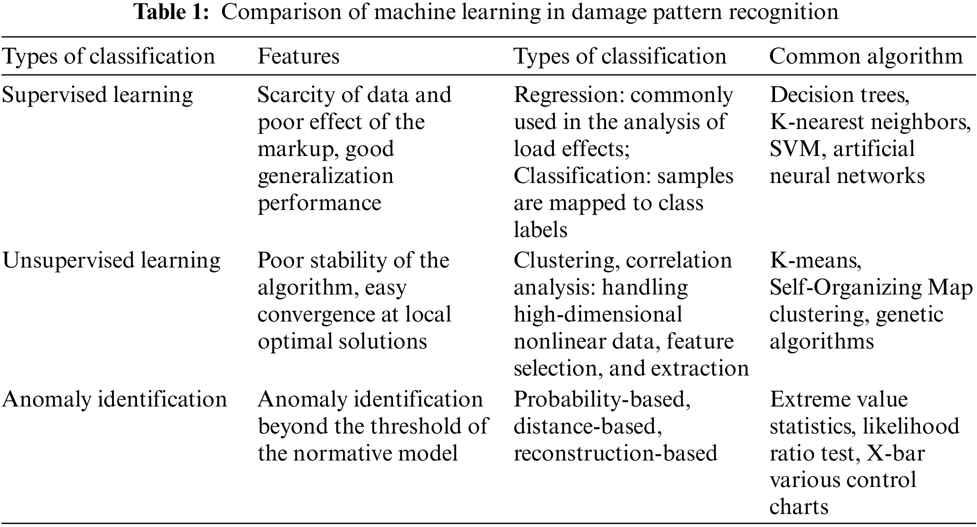
In Table 1, the KNN algorithm has the advantages of being intuitive to understand and able to exploit the local distribution of the data without the need to estimate the whole. Nonetheless, it performs poorly in the degree of conformity between local estimation and global distribution and probability calculating and it is sensitive to the value of K, which easily causes overfitting and underfitting. The K-means clustering algorithm is an unsupervised class of algorithms that do not require sample labeling information. It does not perform as well as supervised learning for not implementing the labeling information of the data. It is also sensitive to the value of K and the sample distribution of the dataset itself [20]. Cart decision tree adopts a binary cut of the data to classify, which has the advantages of intuitive visualization, easy traceability and regression. However, this model is susceptible to the maximum depth of the tree prefabricated parameters, and it is computationally slow and inefficient when dealing with a large quantity and high dimensionality data [21]. Nonlinear Support Vector Machines (SVM) map low-dimensional data to high-dimensional feature space and then segment indistinguishable low-dimensional data with a decision-dividing hyperplane. Nonlinear-SVM is a part of a strong classifier that ensures the greatest possible distinction between two categories. But when dealing with scenarios where multiple categories mix, it is incapable of maintaining the global fault tolerance rate and is vulnerable to kernel function and parameter selection. The neural network is connected layer by layer in terms of weight to regress the complicated distribution. With a large number of internal parameters, the neural network’s nonlinear transformation can match any distribution. Its shortcoming includes sensitivity to changes in network topology, slow training and over-fitting [22]. Generally speaking, a single machine learning model exists with a lot of assumptions, and a very flexible model is easily overfitted. The quantity of data, the speed of training prediction, accuracy, and the complexity of data interpretation must all be taken into account when selecting models, and there is no one-size-fits-all approach.

Since there is a large number of bridges and culverts in the northwest rural areas in China, and municipal funding is limited. It is difficult to install the advanced bridge SHM in those undeveloped area. With respect to the old bridges in rural areas, an affordable system is essential. The goal of this work is to provide a system for identifying old arch bridge deterioration that is quick, inexpensive, and accurate. The suggested approach also has general applicability in assessing the overall condition of various bridge types in rural areas quickly and accurately.

2  Old Arch Bridge Damage Identification System Framework

This paper integrates time-frequency domain feature extraction and Machine Learning (ML) for damage identification. Taking the vehicle’s live load as the environmental excitation, the acceleration sensor measuring points are arranged at different positions of the old arch bridge to collect acceleration mode signals containing damage information. The working principle is presented in Fig. 1. The damage indicators are constructed by combining wavelet packet analysis theory. Then, the random forest algorithm is implemented to make pattern classification and training of a set of old arch bridge data. The technical route of damage identification is illustrated in Fig. 2. After this section, this system will be elaborated in detail from the aspects of energy damage index construction, comparison of ML methods and model optimization.

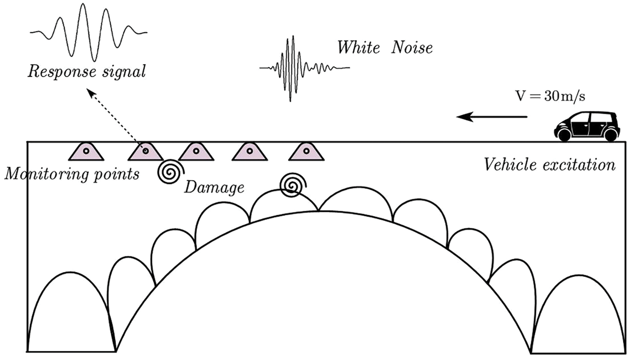
Figure 1: Principle of vehicle-induced vibration response

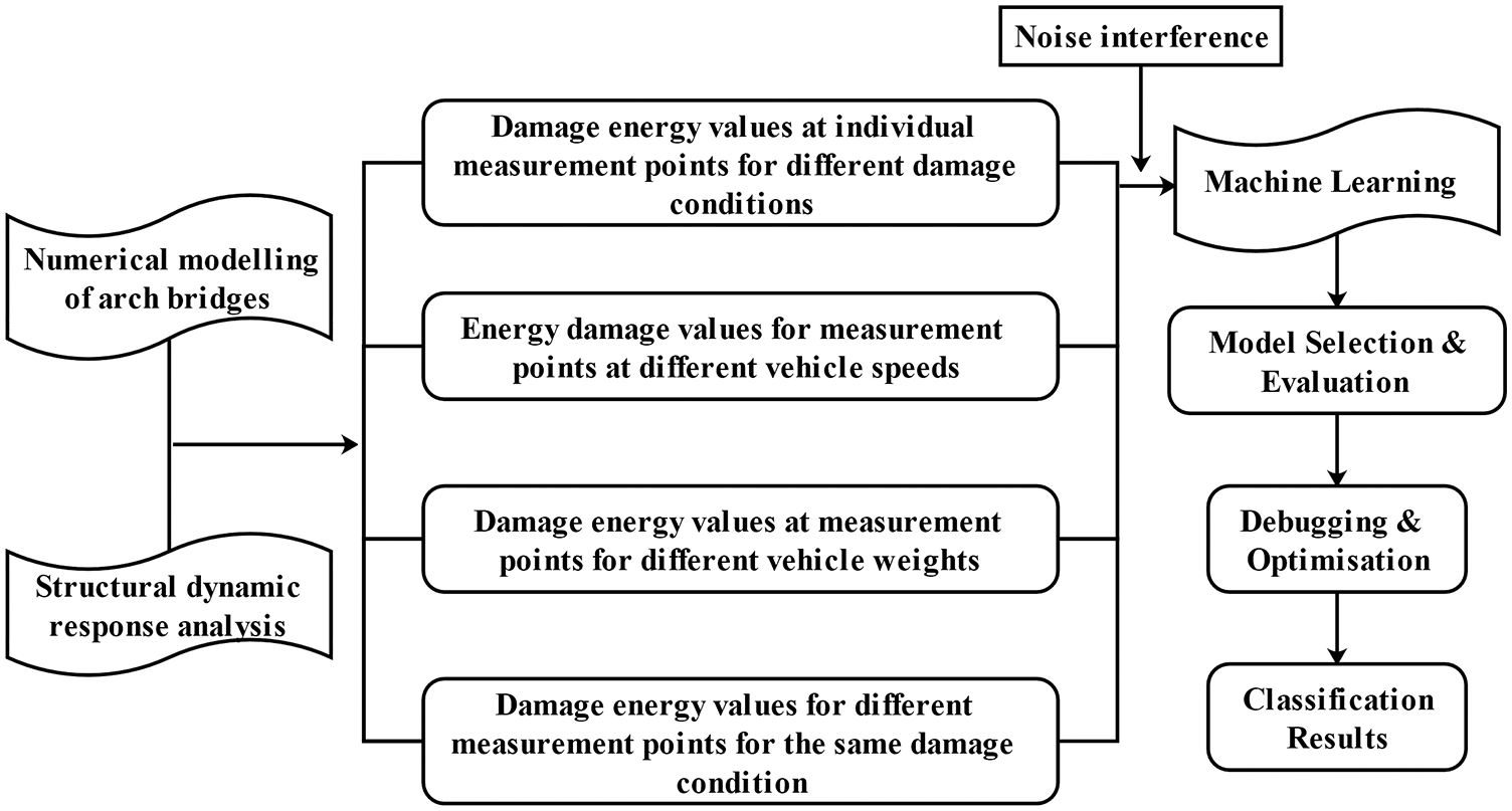
Figure 2: Process of damage identification

3  Construction of Damage Indicators for Old Arch Bridges

3.1 Construction of Wavelet Packet Energy Damage Index

Wavelet analysis only targets the decomposition of the low-frequency part at each scale and the frequency domain resolution in the high-frequency part is insufficient, resulting in partial loss of structural damage information in the high-frequency signal. By further dividing the signal at several scales and identifying features in different time-frequency with stable orthogonal time-frequency properties, wavelet packet analysis allows for improved frequency resolution [23].

Parseval’s theorem states that signal energy is the sum of squares of varying amplitudes. The high and low frequencies are decomposed into frequency bands, and the sum of each band is the signal energy [24]. After decomposing the wavelet packet with a signal scale 2i into i layers, Eq. (1) is obtained, and the signal in each frequency band can be calculated with Eq. (3).

f(t)=∑j=12ifij(t)(1)

where f(t) is the signal, i is the number of decomposition layers, and j is the scale parameter indicating the j wavelet packet of the corresponding layer.

Wavelet packet coefficients can be expressed as:

ci,kj(t)=∫−∞+∞f(t)ui,kj(t)dt(2)

where uα˙,kj(t) and ci,kj(t) are wavelet packet (signal) functions and coefficients.

The decomposed different frequency bands are the equations as follows:

fij(t)=∑−∞+∞ci,kj(t)ui,kj(t)(3)

Ei=∫−∞+∞f(t)2dt=∑m=12i∑n=12i∫−∞+∞fim(t)fin(t)dt(4)

In Eq. (4), where Ei is the accumulated total energy value of wavelet packet energy in different frequency band.

The energy values of distinct signal bands are determined from the orthogonality (Eq. (5)) by combining Eqs. (3) and (4).

Eij=∑j2iEij=∑j2i∫−∞+∞fij(t)2dt(5)

The frequency changes when the signal passes through the damaged part of the old arch bridge, and the energy value will change abruptly. The energy of the components has a high sensitivity to the change of the signal, so the adoption of wavelet packet energy values makes better response to the damage changes to the structure [25].

Defining the wavelet packet energy damage index as Damage Index (DI), which can be expressed as Eq. (6).

DI=∑i=12i−1(dEijhEij−1)2(6)

where hEij is the wavelet packet energy value of signal without damage/healthy condition; dEij is the wavelet packet energy value of signal with the damaged condition; 2i−1 indicates the number of bands of the final wavelet decomposition.

The steps to obtain the wavelet energy damage index are as follows. To begin with, the wavelet packet energy values of health and damage conditions under decomposition scale i were calculated as hEij and dEij, respectively, utilizing the acceleration time-history signal of an arch bridge under various working conditions. The energy change can then be calculated using the difference between the two and the energy change rate can be calculated using the normalized elimination dimension. After signal decomposition, the normalized energy change rate is squared to avoid negative values and reduce the influence of individual bands, and the squared energy change rate of each decomposition band is summed to give the damage index DI.

Wavelet packet analysis is considered because low-scale wavelet decomposition cannot depict the changes before and after structural degradation, according to engineering experience [26]. The original signal is decomposed into three same-band wide-division signals, and the wavelet packet energy of each node is extracted by Eq. (5). The wavelet packet energy of each layer of the damage condition and the corresponding health condition is superimposed by the operation of Eq. (6), which is the wavelet packet energy damage index under this damage condition.

3.2 Response to the Introduction of Data Noise

In the implementation of accelerometers, the inevitable interference of random white noise is mainly from the electromagnetic effect of the accelerometer and the observation error. The noise with a variance of σ2 and a mean value of 0 obeying a normal distribution is called White Gaussian Noise (WGN). The Signal Noise Ratio (SNR, unit: dB) of Eq. (7) is applied to characterize the degree of noise contamination of the acceleration signal, generally speaking, the higher the SNR, the better.

SNR=10log10(σS2σN2)=10log10(SigPowerNoisePower)(7)

In Eq. (7), where σS2,σN2 denote signal variance and noise variance, respectively; SigPower and NoisePower stand for signal power and noise power, respectively (unit: watt W).

4  Random Forest-Based Damage Identification Model for Old Arch Bridge

As the former reviews in Section 1 on the current ML methods described, because there is seldom a parallel method that can be generated simultaneously among individual learners, the Random Forest (R.F.) algorithm technology can be utilized to construct the damage identification model. On the one hand, the model has a high level of randomness and noise resistance, as well as the ability to process high-dimensional data efficiently. Moreover, R.F. is a tree-like structure and the model is deeply interpretable. When modeling the damage identification, training, testing and judgment, the importance of input indexes can be estimated, which is beneficial to the feature selection of damage and has good generalization performance [27,28].

The R.F. algorithm works by randomly extracting multiple sub-samples from the sample database, modeling Cart decision trees for each sub-sample set using the Bootstrap method, which uses reversible random sampling to form different self-help sets. R.F. trains the base classifier’s sampling, and Fig. 3 illustrates how the workflow operates. The outputs of many decision trees are integrated using the regression average method or classified voting method, yielding the best random forest outcomes. The cart decision tree is used as a weak learner; some sample features on nodes are selected by bootstrap sampling. The optimal features are then selected to divide the left and right subtrees of the decision tree.

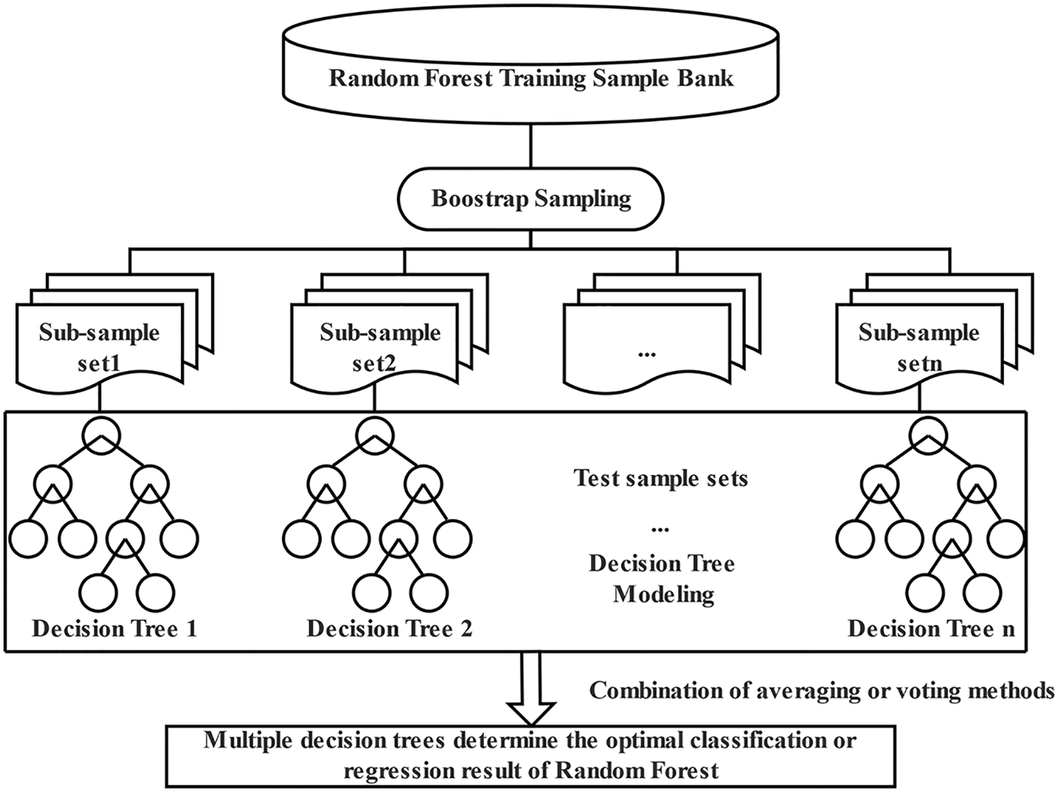
Figure 3: The principle diagram of the random forest modeling

Assuming that εi(x) is the regression result of a single Cart decision tree, the random forest is obtained by the Bootstrap sampling of different sample sets. The decision tree modeling is performed separately to obtain {ε(x,θi),i=1,2,…,n,whereθisrandomvector}. In Eq. (8), the regression type result is obtained after averaging.

ζ(x)=1n∑inεi(x)(8)

where ζ(x) denotes the result of random forest regression.

According to Eq. (9), the subtypes determined from a pool of n samples, are modeled to derive the respective decision tree results and then voted to determine the optimal classification.

ζ(x)=arg maxf⁡∑inη(εi(x)=f)(9)

where ζ(x) denotes the result of random forest classification; εi(x) is the single Cart decision tree output; η(t) is the indicative function; f is the dependent variable.

Each Cart classification decision tree model εl(x),ε2(x),…,εi(x) is Bootstrap randomly sampled from the original large sample pool, and a margin function M(x,f) is introduced to indicate the degree to which the average number of classifications passes more than rejects. Among them, the larger the function value is, the more accurate the classification result is.

M(x,f)=avnη(εi(x)=f)−maxm≠n⁡avnη(εi(x)=m)(10)

Eq. (11) reveals the Generalization Error (G.E.), which represents the model’s ability to generalize.

GE=Pxf(M(x,f)<0)(11)

εi(x)=f(x,θn) obeys the law of strong numbers, and G.E. will converge to the upper bound when the number of branching steps of the Cart decision tree increases, as shown in Eq. (12), furtherly illustrating the robustness of the model without overfitting.

limk→∞⁡GE=Pxf((n(x,θ)=f)−maxPθ(n(x,θ)=m)<0)(12)

where k denotes the number of Cart decision trees.

When the random forest generates the Cart decision tree combination without pruning through Bootstrap sampling, the probability of not being extracted is Pn when the sample size n is large enough:

Pn=limn→∞(1−1n)n=1e=0.367879(13)

According to Eq. (13), 36.8% of the data will not appear in Bootstrap samples, in other words, Out of Bag (OOB) data is generally used to evaluate the model’s generalization ability. The model is a generalized error estimate because each cart decision tree has an OOB error estimate based on all average values. OOB is an unbiased estimation that is not only more efficient but also better than other methods such as cross-validation, just like the test set with the same sample size.

Defining all kinds of sets in the sample library as features, and feature selection is to remove irrelevant features from all features extracted from the sample library, which are connected to the selection of target variables. The curse of dimensionality is mitigated by feature selection, which decreases the difficulty of the learning task and the training time. For example, in terms of the KNN algorithm model, the distribution of samples in space is sparse when the number of indicators is large, which means less effective. At present, feature selection includes the Relieff algorithm, neighborhood component analysis algorithm and mRMR algorithm [29].

The R.F. has superiority on screening the importance of indexes to select features. The Gini value is employed to evaluate the accuracy of determining the random forest algorithm. The concept is that noise is introduced into features, and then the importance of those features is determined by a sudden change in Gini value. Testing the performance with OOB data and comparing it to the old OOB accuracy, the random forest performance is tested after artificially adding noise to the characteristic variables. At last, the new OOB accuracy is obtained. The characteristic variable measurement value is the difference between the old and new OOB accuracy. The importance indexes are screened out during the construction of the arch bridge damage model so that the damage identification model with a large amount of samples can be modified and the model's accuracy can be improved.

5  Case Studies

5.1 Numerical Model of Arch Bridges

The damage of two old arch bridges was assessed using the damage assessment method based on the R.F. algorithm, and the damage identification process of the old arch bridge under vehicle-induced response was simulated by the finite element software CSiBridge.

The entire bridge was discreted as beam element, as demonstrated in Fig. 4. The arch ribs and bridge deck were connected by link element, the initial loading case was uniform dead load and the boundary condition of the arch was constrained.

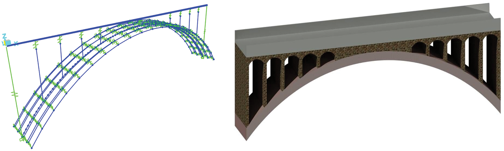
Figure 4: Finite element model of the arch bridge with a span of 50 m

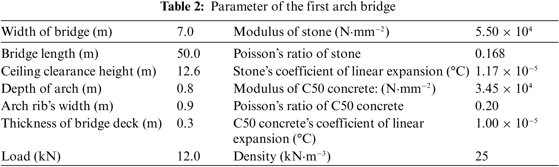
C50 concrete was used in the main arch ribs, arch tile, bridge deck, and cross-linked, and stone was used for the web arch cross-wall in the old arch bridge’s material selection. The material parameters, such as modulus of elasticity, Poisson’s ratio, and bridge type parameters, are summarized in Table 2.

The second arch bridge was made up of two 13 meters approach span and 45 meters main span. The main arch was a constant section with a simply-supported pillar on the arch. The arch was a single box section with five chambers, and its dimension was: a height of 1.2 m, a total width of 7 m and a net height of 5.4 m. The arch was made of C30 concrete, and the roadway was 12 meters wide with one flexible lane of 3.5 meters wide, one non-motorway lane of 1.5 meters wide and one sidewalk in each direction. The specific modeling process is similar to the first bridge, and Fig. 5 depicts the geometric model.

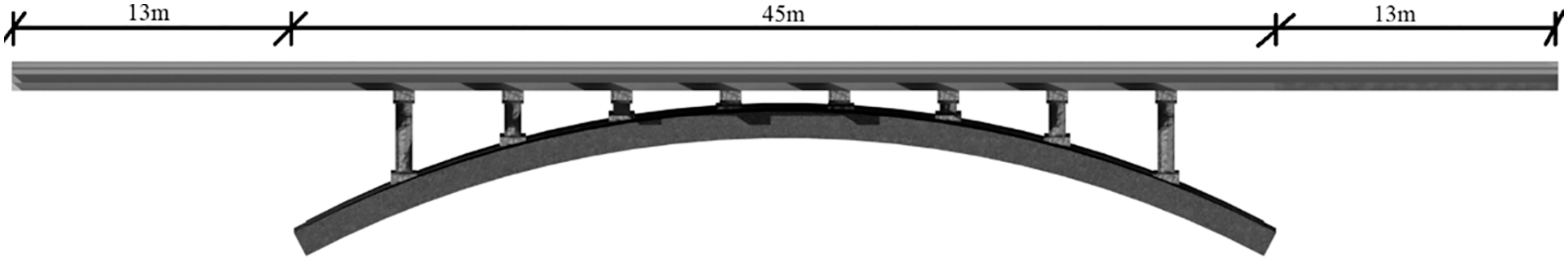
Figure 5: Geometric model of the arch bridge with a span of 45 m

In CSiBridge, it provided the vehicle load function. The front and rear axle spacing was 3 m, both axles weighed 750 kg, the front axle weighed 1560 kg and the rear axle weighed 1820 kg of the two types of vehicle concentrated force live load. The above vehicles are the typical traffic flows at the bridge location, and the vehicle selection is consistent with the actual situation. The vehicle was set to pass over the arch bridge at a constant speed of 30, 40 and 50 km/h respectively in the load section.

5.2 Arrangement of Measuring Points

The vehicle-bridge coupling analysis of a 50 m-span hyperbolic arch bridge is carried out in the finite element software CSiBridge to improve the layout of the test process and establish the location control of the acceleration sensor. The arch bridge is loaded with a live car with double axles of 7.5 KN and axle spacing of 1.5 m. The vehicle passes through at speeds of 10, 15 and 20 m/s per second. The fast Fourier transform is applied to the acceleration time-history response, and the amplitude peaks of each point are compared. The sensor measurement point’s control position is set to the maximum node energy.

In the entire bridge, 19 nodes are picked for comparison. Fig. 6 depicts the acceleration vibration mode curves of each node at various vehicle speeds. In order to distinguish easily, the acceleration vibration mode curves of each node at various vehicle speeds are represented by curves in different colors. Because the time domain signal is indivisible, it was carried on the frequency domain analysis.

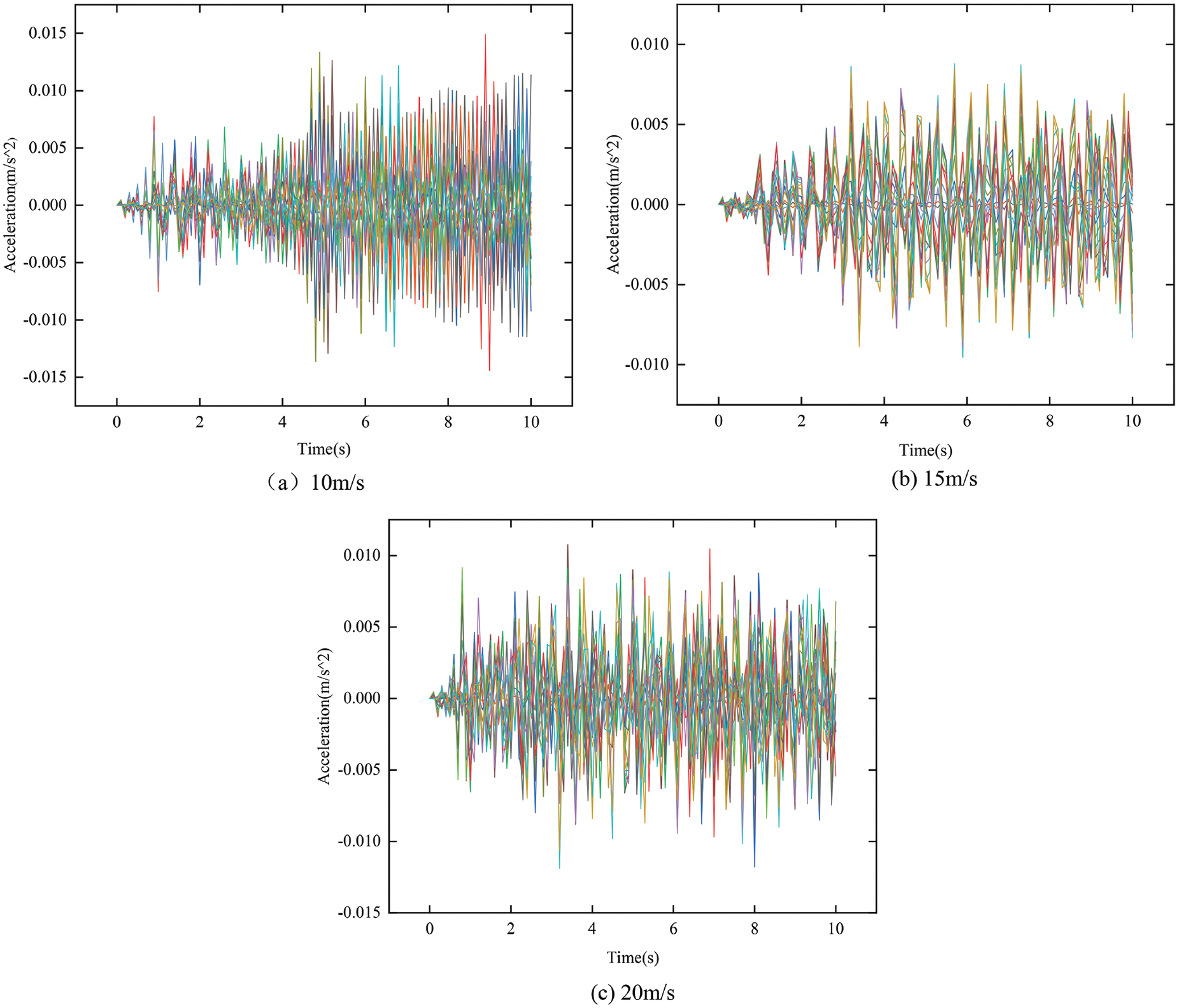
Figure 6: The acceleration vibration mode curve of each node

FFT is applied to a time-domain curve with a vehicle speed of 15 m/s and a sampling frequency of 10 s, which satisfies the sampling theorem. As shown in Fig. 7, the acceleration response spectrum is obtained. Fig. 7a depicts the layout of the bridge's 19 measuring points. Fig. 7b shows the FFT results for measuring point 6, and Fig. 7c shows the comparison result after selecting each measuring point’s maximum spectrum peak. The results show that the response peaks of measuring points 5–9, 13, 14, 17 and 18 are the largest among the amplitude of acceleration response spectrum under different vehicle speeds, and the damage energy of energy index is the maximum value of each point of the entire bridge after calculation.

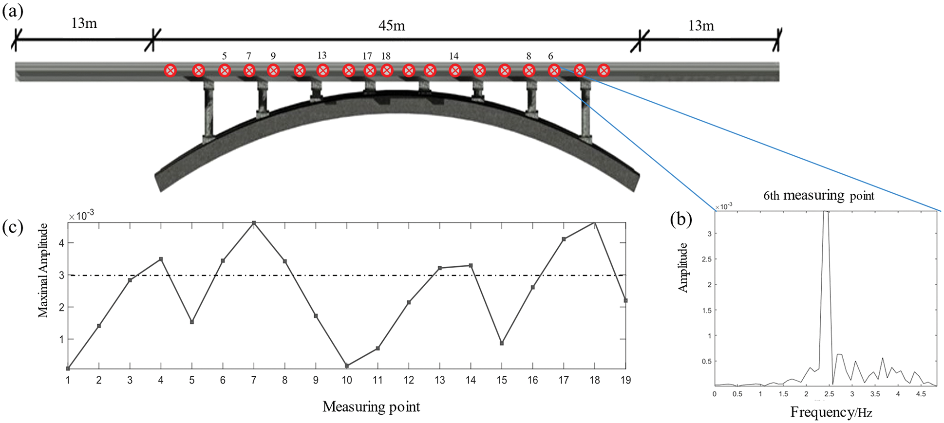
Figure 7: Acceleration measuring point-FFT spectrum peak

In most cases, the meso-damage of in-service arch bridge is hard to detect. After decades of weathering, material degradation and the accumulation of the meso-damage, the local stiffness of the arch bridge in the damaged region will change dramatically. From this perspective, the level of component’s damage and different damage conditions can be simulated by the stiffness degradation of the element. The greatest amplitude peak of the spectrum position is chosen as the measuring point of the acceleration sensor. On the arch bridge, five measuring spots with the highest response amplitude in the acceleration spectrum map are determined as demonstrating in Fig. 8.

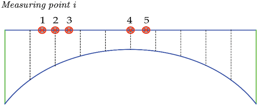
Figure 8: Arrangement of measuring points

5.3 Control Variables and Simulation Loading

5.3.1 Loading Simulation for Different Damage Conditions

Each measurement point in the model has a 10 s acceleration sampling time and a frequency of 100 Hz. Simulating damage conditions of 10%, 20% and 30% for the third measurement point, while simulating the healthy working condition mode of the No. 3 measurement point. The vehicle with a front axle load of 1560 kg and rear axle load of 1820 kg passed through the arch bridge at a speed of 30 km/h and produced six-dimensional accelerations: the translational acceleration of the XYZ axis and the acceleration of rotation around each axis. These records were exported to Matlab for time-frequency domain analysis, and the acceleration of each dimension was operated as Eq. (14) to obtain the combined acceleration:

Mag=x2+y2+z2+a2+b2+c2(14)

where Mag represents convergent acceleration, x, y, z represents translational acceleration, and a, b, c represents rotational acceleration.

The combined acceleration time-history response curve under different damage conditions is plotted in Fig. 9. As the degree of damage continues increasing in Fig. 9, the maximum amplitude of the acceleration ascends simultaneously. Similarly, the vehicle weight, loading speed and axle weight were kept constant, and the acceleration time-history response with the damage conditions of 10%, 20% and 30% have been simulated respectively at the 5 measurement points.

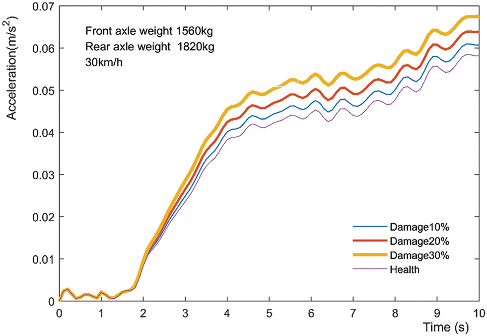
Figure 9: The acceleration vibration curve of 30 km/h measuring point 3 for different damage conditions

5.3.2 Calculation of Data Noise

The signal has been frequently disrupted by noise during the field test and recording. Gaussian white noise with signal-to-noise ratio magnitudes of about 33 and 53 dB has been applied to the acceleration response signals to guarantee that the trained numerical model reflects the same characteristics as the real field test [30]. At a speed of 30 km/h, the vehicle with a front axle load of 1560 kg and a rear axle load of 1820 kg passed through the arch bridge. The white Gaussian noise with SNR of 33 and 53 dB were introduced to the acceleration time-history response under this condition. The comparison time-history diagram of the original signal and the noise signal at the point 3 is drawn in Fig. 10, in which as the signal-to-noise ratio SNR decreases the amplitude of the curve oscillation increases. To put it another way, more of the original signal would be submerged in noise.

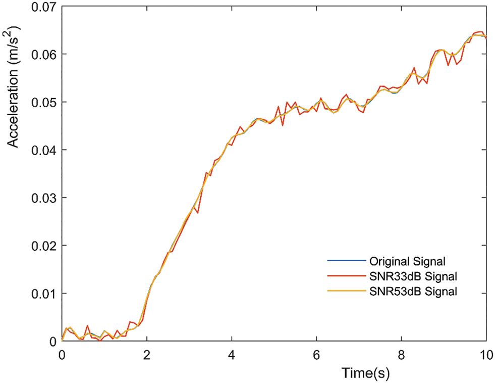
Figure 10: Comparison between the original signal and introduced noise signal

To ensure the balance of the samples, the amplitude of the same order of magnitude as the original signal, 96 groups of white Gaussian noise with SNR size of 53, 73 and 93 dB were introduced to various damage conditions, vehicle speed and load condition, while calculating the wavelet packet energy damage values under the corresponding conditions.

5.3.3 Damage Energy Values under Different Conditions

The damage conditions of each point and the remaining parameters were kept constant by uniformly applying two types of vehicle load and three types of speed through the arch bridge as demonstrated in Eq. (15). Different conditions were used to simulate the acceleration time-history response curve. Indeed, the time-history response under different damage conditions was calculated for a total of 450 groups, and the response data under healthy conditions was 30 groups, yielding a total of 480 groups:

(Speed[123]×Axleweight[12]×pointdamage[12345]×damage[10%20%30%])×point[12345]=damageresponse(450groups)

(Speed[ 123 ]×Axleweight[ 12 ]×health)×point[ 12345 ]=health response(30groups)(15)

The wavelet packet 2N decomposition of DB20 was performed in Matlab on the 5 measuring points representing health status and three damage conditions under various vehicle and speed conditions. After that, the corresponding layers were superimposed by Eqs. (13) and (15). Lastly, the damage energy value of 450 groups of wavelet packs was obtained, plus the energy value of 30 groups of health conditions, a total of 480 sets of DI values. The simulated loading and measurement point arrangement process of the second arch bridge was the same as that of the first arch bridge. The two bridges had a total of 960 sets of DI values. The operation flow is demonstrated in Fig. 11.

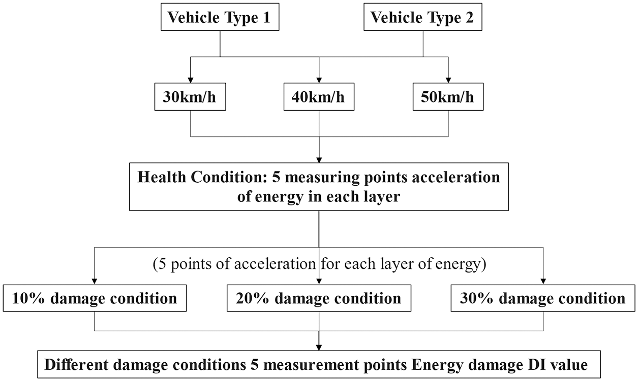
Figure 11: Calculation flow of damage energy DI value of each measuring point under different conditions

6  Evaluation and Comparison of Algorithms

6.1 Evaluation Indicators

The four typical classification indexes T.P., F.N., F.P., and T.N. that define the positive class are shown in Table 3:

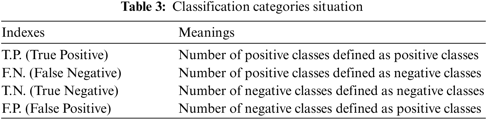
The most common classification of rating models includes accuracy, Micro/Macro F1 score, True Positive Rate (TPR), False Positive Rate (FPR), Receiver Operating Characteristic (ROC) curve, and Area Under Curve (AUC) [31]. The model's classification accuracy is defined as correctly identifying the proportion of the number of samples to the total sample, denoted by Ac; R/TPR denotes the complete rate or the percentage of the sample classified as a positive class. Negative classes are incorrectly classified as positives, according to FPR. The number represents the percentage of the total negative sample; the accuracy rate is expressed in P or classification accuracy. The proportions are correctly classified in a sample of positive classes [32]. The F1 score is defined as the mean of the harmony of the complete rate, the accuracy rate, and the value range, with the larger value indicating a better classification effect. Micro F1 finds the corresponding total check rate and accuracy rate values for each group, then adjusts the average number to obtain; Macro F1 is the average of the F1 scores under different damage conditions. Eq. (16) explains how each indicator is calculated.

Ac=(TP+TN)(TP+FN+TN+FP)

R(TPR)=TPTP+FNFPR=FPFP+TN(16)

P=TPTP+FPF1=2TP2TP+FP+FN

With the true class rate TPR as the vertical coordinate and the false-positive class rate FPR as the horizontal coordinate, the ROC curve represents a curve drawn from a series of different classification thresholds. The larger the FPR, the more actual negative classes in the positive class are predicted, while the larger the TPR, the more actual positive classes in positive classes are predicted. Ideally, the true class rate TPR is close to 1 and FPR is close to 0, which means that the closer the ROC curve is to (0, 1) and the more it deviates from the 45 degrees diagonal, the better the classification effect of the model is. In the multi-classification problem of damage identification, the ROC curves are finally averaged by combining two and two with different damage levels. In the actual analysis, if multiple ROC curves intersect, it is difficult to judge the model's merit. Hence, the AUC value is introduced, which is the area enclosed by the ROC curve and the axis below (the value range is [0,1]).

6.2 Construction of the Sample Library

In this study, the numerical simulation results were used as the test training set to construct a sample library of old arch bridge damage identification for classification learning, testing and evaluation.

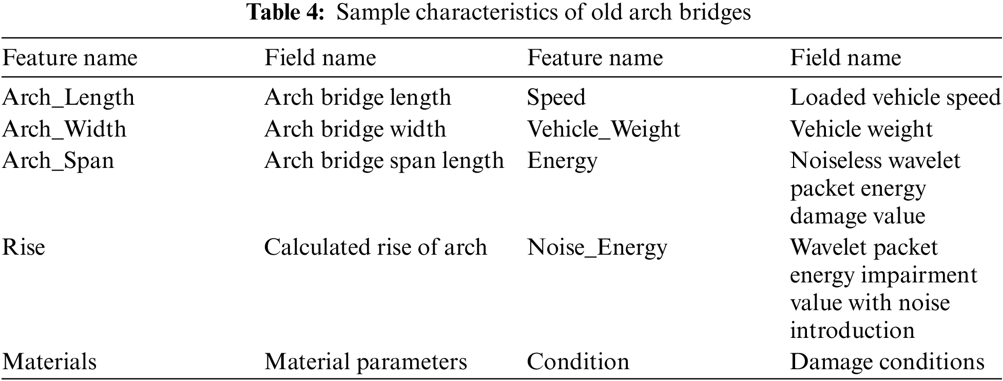
It is necessary to clean and standardize the sample data source because it will appear in various discrete and continuous forms. As shown in Table 4, these sample characteristics of the old arch bridge are involved: the arch bridge width, span length, the material parameters, the loading speed, vehicle weight, the energy damage value with different noises, and the energy damage value without noise etc.

For machine learning in the latter section, the sample library has been trained with random forest and compared to other algorithmic models.

6.3 Comparison of Different Model Algorithms

The training results of random forest are compared with BPNN, the SVM algorithm model. The training of the BPNN belongs to gradient descent, using Cross-Entropy as the loss function. The smaller the learning rate, the better, but it brings longer training. The SVM chooses the Radial Basis Function (RBF) as kernel function [33], due to the linear indivisibility of the data, and to prevent the model from overfitting, a grid search is used for hyperparameter tuning to find the optimal penalty factor c and stop training error g. The number of split features and the number of subtree trees are two important R.F. parameters that are empirically initialized. Multiple pieces of training are used to obtain the optimal parameters of each model, ensuring the robustness of the models. Table 5 presents a comparison of the three models on the test set.

The ROC curves of the three are plotted and the corresponding AUC values have been derived. As displayed in Table 5 and Fig. 12, the R.F. accuracy, F1 score, AUC values, and ROC curves all performed better than B.P. neural network and SVM support vector machine, and the R.F. damage recognition model had a stronger damage recognition ability.

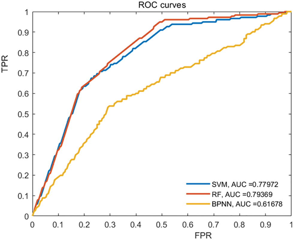
Figure 12: Comparison of ROC curve and AUC value

7  Optimization of R.F. Models

7.1 Optimization Theory of Particle Swarm Algorithms

To improve the accuracy of the random forest damage recognition model, two important parameters of the random forest, the number of split features and the number of sub-trees, are hyperparameter tuned. Traditional grid search will traverse a variety of situations, parameter optimization is relatively blind, the calculation time is long, and the use of heuristic search algorithms can accelerate the solution and find the optimal solution.

Four popular algorithms have been compared: PSO (Particle Swarm Optimization Algorithms), WOA (Whale Optimization Algorithms), MFO (Moth Flame Optimization), and G.A. (Genetic Algorithm). Firstly, the MFO has the disadvantage of getting into the local best and the convergence rate cannot be satisfying [34].

Secondly, the G.A. algorithm has not been able to use the feedback information of the network in time. At the same time, the realization of the three operators also has many parameters, such as crossover rate and mutation rate, and the selection of these parameters seriously affects the solution. At present, the selection of these parameters is mostly based on experience. The PSO algorithm implemented in this paper can use inertia weight and learning factor gradient to prevent dependence on empirical parameters [35].

Thirdly, WOA whale converges slowly in the search process, and it is easy to fall into local optimum in the update mechanism, which restricts the classification performance and dimensionality reduction of the algorithm [36]. To conclude, PSO particle swarm algorithm is easy to understand, and the algorithm is stable, especially when searching for multiple parameters.

The particle search process is divided into three parts: search inertia, self, and other group search experiences. Particle local optimal position gbesti,dk and global optimal position pbesti,dk are constantly updated in the search space based on particle fitness. In the particle iteration, Eq. (17) calculates the velocity, and Eq. (18) calculates the coordinates.

vi,dk=wkvi,dk−1+c1kr1(pbesti,dk−xi,dk)+c2kr2(gbesti,dk−xi,dk)(17)

where vi,dk is the velocity of the ith particle in the d dimension at k iterations; wk is the inertia weight at k iterations; c1k,c2k represent the individual learning factor and group learning factor at k iterations; r1,r2 are random numbers on the interval [0,1]; pbesti,dk , gbesti,dk represent the local optimum and the global optimum of the ith particle in the d dimension.

xi,dk+1=xi,dk+vi,dk(18)

where xi,dk+1 represents the position of the ith particle in dimension d at k iterations.

By changing the inertia weights and the individual or group learning factors [37,38], the global and local iterative optimization search process of the PSO algorithm can be better balanced to prevent falling into local extremum points. Eq. (19) utilizes linearly decreasing inertia weight values, and Eq. (20) calculates asymmetric individual and group learning factors, with a larger inertia weight value favoring global search in the early stages and a smaller value favoring local search in the later stages.

wk=wstart −(wstart −wend )×kKmax(19)

c1k=c1start +(c1end −c1start )×kKmax

c2k=c2start +(c2end −c2start )×kKmax(20)

where wstart and wend represent the initial (maximum) and termination (minimum) inertia weight values; k is the number of current iterations; Kmax is the total number of iterations; c1start and c1end represent the initial and final values of the individual learning factor; c2start and c2end represent the initial and final values of the group learning factor.

7.2 PSO Optimized R.F. Damage Identification Model

The arch bridge’s damage output consisted of three damage conditions. The PSO optimized R.F. damage identification model was designed to evaluate hyperparameter selection and characterize the model’s damage identification performance. The damage identification was evaluated in terms of overall accuracy and the proportion of sample data with accurate identification of the three damage conditions to all samples. Fig. 13 depicts how the particle swarm algorithm optimizes the random forest damage recognition model.

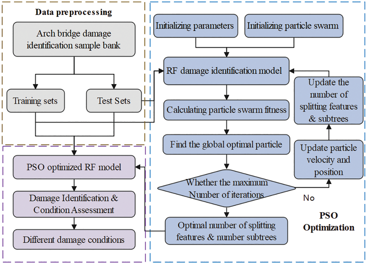
Figure 13: PSO-RF damage identification model

The data sample pool was divided into training and test sets with an 8:2 ratio, and the model was tested with random sequence labels before PSO optimization. Observed from Fig. 13, the particle swarm parameters were first initialized, such as the maximum number of iterations, the range of particle parameters (number of subtrees & split features), individual and group learning factors and inertia weights. Moreover, this training set was used to train the R.F. damage recognition model, and the accuracy of damage recognition was evaluated with the test set, and the fitness value of particles was calculated from the accuracy. The velocity and position of the particle swarm were iterated continuously from Eqs. (17) to (20), and the number of split features and subtrees of R.F. were updated to make the best fitness of individuals and groups. The highest accuracy was obtained until the maximum number of iterations was reached and terminated. The global optimal number of splitting features and subtrees was obtained. Finally, the optimized PSO-RF model was used for damage identification and model evaluation.

7.3 Analysis of Optimization Results

The iterative process of optimizing parameters of the R.F. algorithm is depicted in Fig. 14, in which the number of subtrees, the number of splitting features and the particle fitness utilized the PSO algorithm terminates after six rounds of 100 iterations. Two of the optimized parameters reach the optimal values in the 62nd, 21st, 87th, 9th, 47th, and 12th iterations from rounds 1 to 6. From 97.2% or 97.8% to the optimal value of 98.3%, the PSO optimization process goes through 1–3 stages to achieve the optimal value, which further demonstrates the stable classification performance of the R.F. model.

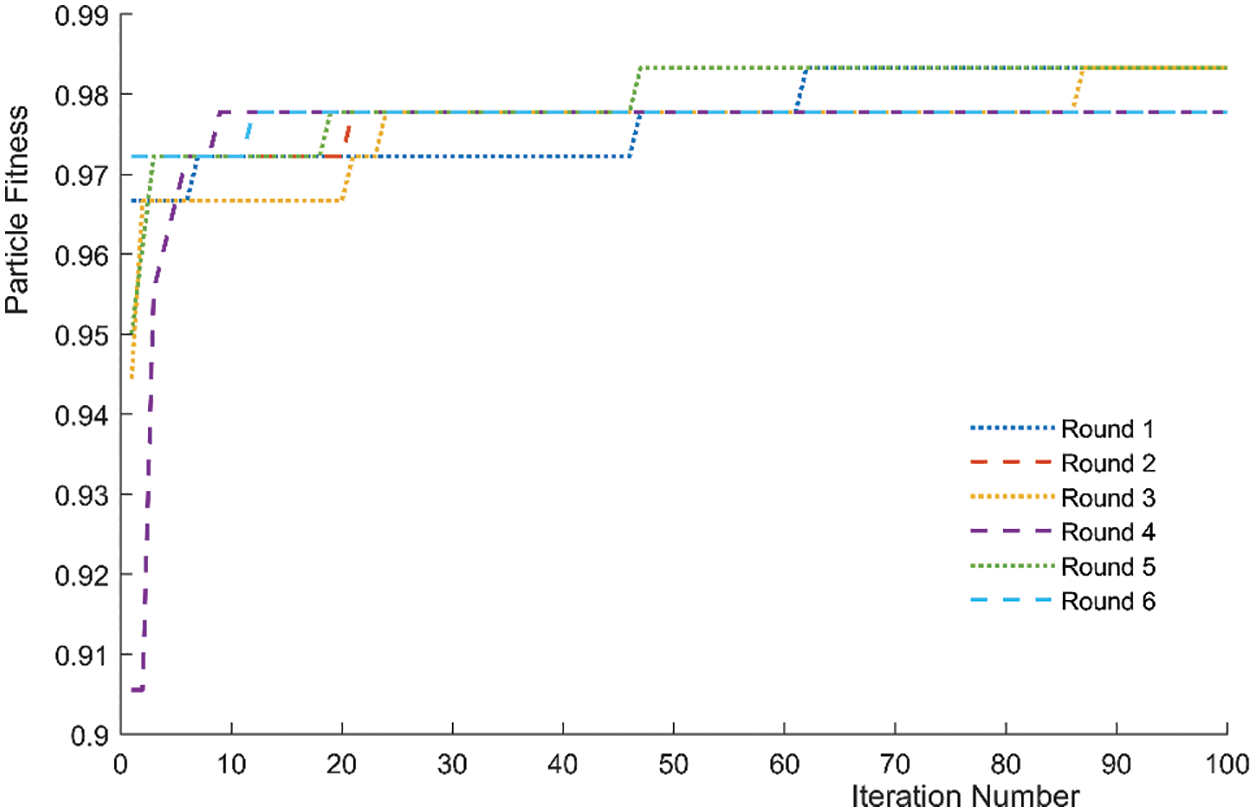
Figure 14: Particle swarm fitness iterative process

After iterations, the parameter combinations of multiple optimal R.F. models were obtained, the number of split features and the number of subtree trees with the most intensive occurrence 3 and 149 were taken, and the optimal fitness of the particles was 98.3%. The classification accuracy of PSO-RF was 95.6%, 95.6% and 95.6% for Micro F1 and Macro F1, and all indicators were higher than the other three types of models.

Feature selection has been utilized to identify the significant characteristics. The selected features contain physical quantities such as damage indications. Comparing the important features of R.F. and PSO-RF models in Fig. 15, where the feature in the range of 8~13 is much higher than other feature terms. This proves the significance of the proposed DI and the sensitivity of indicators. It is also observed that the original signal damage identification features in PSO-RF present higher feature importance.

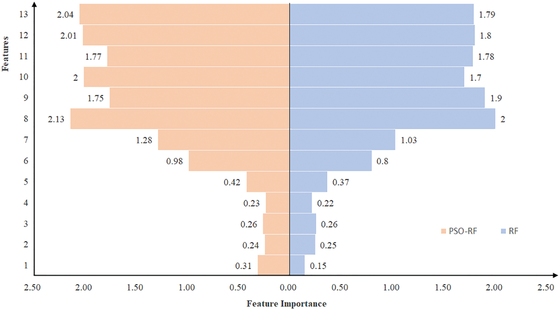
Figure 15: Feature importance of R.F. and PSO-RF

8  Conclusions

In this research, a fast structural damage identification framework based on machine learning is proposed, which aims to address the problem of rural regions’ old bridge maintenance. Three different machine learning approaches-BPNN, SVM and R.F. have been compared in the evaluation of the damage status of old arch bridges. The following conclusions can be drawn:

(1)   The study simulates a numerical damage model in the environment with field noise, then trains an R.F. model according to the simulated 960 sets of data. The proposed damage identification index performs optimally in terms of feature importance in the R.F. damage identification model, and it plays an important role during the selection of important features.

(2)   The R.F. model has a 35 percent and 8.4 percent higher precision than SVM and BPNN, respectively, and a 34.9 percent and 8.4 percent higher index F1 score. R.F.’s Auc value is 2 percent higher and 17.7 percent greater than both SVM and BPNN. The constructed RF damage identification model has a better recognition capability compared with BPNN and SVM.

(3)   The two hyperparameters of RF, the number of split features and subtrees have been optimized by the PSO algorithm, which avoids the problem of selecting empirical parameters that make the model classification unreliable and improves the accuracy of the model.

The proposed framework can also be easily extended to other bridge types, such as the prestressed concrete girder bridge, which has a general validity to the rapid and accurate assessment of the overall state of different bridge types in rural regions.

Author Contributions: Conceptualization, Z. X., and Y. Z.; methodology, Y. Z., and Z. X.; software, J. S., Z. L and Y. Z.; validation, Z. X., Y. Z., and J. S.; formal analysis, Y. Z., and J. S.; investigation, J. S., C. M. and Y. Z.; resources, Z. X., Z. L, Y. Z. and J. S.; data curation, Y. Z., J. S., and Z. X.; writing—original draft preparation, Y. Z, J. S., and Z. X.; writing—review and editing, Y. Z., Z. L and Z. X.; visualization, Y. Z. and J. S.; supervision, Z. X.; funding acquisition, Z. X., J. S., and Y. Z. All authors have read and agreed to the published version of the manuscript.

Funding Statement: This study and the related research were financially supported by the Elite Scholar Program of Northwest A&F University (Grant No. Z111022001), the Research Fund of Department of Transport of Shannxi Province (Grant No. 22-23K), the Student Innovation and Entrepreneurship Training Program of China (Project Nos. S202110712555 and S202110712534).

Conflicts of Interest: The authors declare that they have no conflicts of interest to report regarding the present study.

References

1. Zhang, Y., Xiong, Z., Luo, J., Luo, J., Zhu, H. (2021). Construction of rapid evaluation system of old stone arch bridge in Shaanxi Province. Journal of Water Resources and Architectural Engineering, 19(4), 168–174 (in Chinese). DOI 10.3969/j.issn.1672-1144.2021.04.027. [Google Scholar] [CrossRef]
2. Xiong, Z., Li, J., Zhu, H., Liu, X., Liang, Z. (2022). Ultimate bending strength evaluation of MVFT composite girder by using finite element method and machine learning regressors. Latin American Journal of Solids and Structures, 19(3), 1308. DOI 10.1590/1679-78257006. [Google Scholar] [CrossRef]
3. Avci, O., Abdeljaber, O., Kiranyaz, S., Hussein, M., Gabbouj, M. et al. (2021). A review of vibration-based damage detection in civil structures: From traditional methods to Machine Learning and Deep Learning applications. Mechanical Systems and Signal Processing, 147, 107077. DOI 10.1016/j.ymssp.2020.107077. [Google Scholar] [CrossRef]
4. Mangalathu, S., Hwang, S. H., Choi, E., Jeon, J. S. (2019). Rapid seismic damage evaluation of bridge portfolios using machine learning techniques. Engineering Structures, 201, 109785. DOI 10.1016/j.engstruct.2019.109785. [Google Scholar] [CrossRef]
5. Gandomi, A. H., Chen, F., Abualigah, L. (2022). Machine learning technologies for big data analytics. Electronics, 11(3), 421. DOI 10.3390/electronics11030421. [Google Scholar] [CrossRef]
6. Naser, M. Z., Alavi, A. H. (2021). Error metrics and performance fitness indicators for artificial intelligence and machine learning in engineering and sciences. Architecture, Structures and Construction, 14, 1–19. DOI 10.1007/s44150-021-00015-8. [Google Scholar] [CrossRef]
7. Kurian, B., Liyanapathirana, R. (2020). Machine learning techniques for structural health monitoring. Proceedings of the 13th International Conference on Damage Assessment of Structures, pp. 3–24. Singapore. DOI 10.1007/978-981-13-8331-1_1. [Google Scholar] [CrossRef]
8. Thai, H. T. (2022). Machine learning for structural engineering: A state-of-the-art review. Structures, 38, 448–491. DOI 10.1016/j.istruc.2022.02.003. [Google Scholar] [CrossRef]
9. Fu, Y., Peng, C., Gomez, F., Narazaki, Y., Spencer Jr, B. F. (2019). Sensor fault management techniques for wireless smart sensor networks in structural health monitoring. Structural Control and Health Monitoring, 26(7), e2362. DOI 10.1002/stc.2362. [Google Scholar] [CrossRef]
10. Zhang, E., Shan, D., Li, Q. (2019). Nonlinear and non-stationary detection for measured dynamic signal from bridge structure based on adaptive decomposition and multiscale recurrence analysis. Applied Sciences, 9(7), 1302. DOI 10.3390/app9071302. [Google Scholar] [CrossRef]
11. Shan, D. S., Li, Q., Huang, Z. (2015). Adaptive decomposition and reconstruction for bridge structural dynamic testing signals. Journal of Vibration and Shock, 34(3) (in Chinese). DOI 10.13465/j.cnki.jvs.2015.03.001. [Google Scholar] [CrossRef]
12. Do, N. T., Gül, M. (2020). A time series based damage detection method for obtaining separate mass and stiffness damage features of shear-type structures. Engineering Structures, 208(2), 109914. DOI 10.1016/j.engstruct.2019.109914. [Google Scholar] [CrossRef]
13. Ni, Y. Q., Wang, Y. W., Zhang, C. (2020). A Bayesian approach for condition assessment and damage alarm of bridge expansion joints using long-term structural health monitoring data. Engineering Structures, 212(1), 110520. DOI 10.1016/j.engstruct.2020.110520. [Google Scholar] [CrossRef]
14. Noori, M., Wang, H., Altabey, W. A., Silik, A. I. (2018). A modified wavelet energy rate-based damage identification method for steel bridges. Scientia Iranica, 25(6), 3210–3230. DOI 10.24200/sci.2018.20736. [Google Scholar] [CrossRef]
15. Yan, Y., Zhan, J., Zhang, N., Xia, H., Li, M. et al. (2018). A damage evaluation method for simply-supported bridges based on wavelet transform correlation. Journal of Vibration and Shock, 37(12), 67–74 (in Chinese). DOI 10.13465/j.cnki.jvs.2018.12.011. [Google Scholar] [CrossRef]
16. Ni, F., Zhang, J., Noori, M. N. (2020). Deep learning for data anomaly detection and data compression of a long-span suspension bridge. Computer-Aided Civil and Infrastructure Engineering, 35(7), 685–700. DOI 10.1111/mice.12528. [Google Scholar] [CrossRef]
17. Guo, A., Jiang, A., Lin, J., Li, X. (2020). Data mining algorithms for bridge health monitoring: Kohonen clustering and LSTM prediction approaches. The Journal of Supercomputing, 76(2), 932–947. DOI 10.1007/s11227-019-03045-8. [Google Scholar] [CrossRef]
18. Assaad, R., El-adaway, I. H. (2020). Bridge infrastructure asset management system: Comparative computational machine learning approach for evaluating and predicting deck deterioration conditions. Journal of Infrastructure Systems, 26(3), 04020032. DOI 10.1061/(ASCE)IS.1943-555X.0000572. [Google Scholar] [CrossRef]
19. Sun, L. M., Shang, Z. Q., Xia, Y. (2019). Development and prospect of bridge structural health monitoring in the context of big data. China Journal of Highway and Transport, 32(11), 1–20 (in Chinese). DOI 10.19721/j.cnki.1001-7372.2019.11.001. [Google Scholar] [CrossRef]
20. Yu, W., Xu, L. Y. (2016). Research on text categorization of KNN based on K-means for class imbalanced problem. Sixth International Conference on Instrumentation & Measurement, Computer, Communication and Control (IMCCC), pp. 579–583. Harbin, China, IEEE. [Google Scholar]
21. Al-Tashi, Q., Abdulkadir, S. J., Rais, H. M., Mirjalili, S., Alhussian, H. (2020). Approaches to multi-objective feature selection: A systematic literature review. IEEE Access, 8, 125076–125096. DOI 10.1109/access.2020.3007291. [Google Scholar] [CrossRef]
22. Avci, O., Abdeljaber, O., Kiranyaz, S., Hussein, M., Gabbouj, M. et al. (2021). A review of vibration-based damage detection in civil structures: From traditional methods to Machine Learning and Deep Learning applications. Mechanical Systems and Signal Processing, 147, 107077. DOI 10.1016/j.ymssp.2020.107077. [Google Scholar] [CrossRef]
23. Guo, J., Sun, B. N. (2005). Multi-scale analysis based on wavelet transform in bridge health monitoring. Journal of Zhejiang University (Engineering Science), 39, 114–119 (in Chinese). DOI 10.3785/j.issn.1008-973X.2005.01.021. [Google Scholar] [CrossRef]
24. Pan, Y., Zhang, L. M., Wu, X. G., Zhang, K. N., Skibniewski, M. J. (2019). Structural health monitoring and assessment using wavelet packet energy spectrum. Safety Science, 120(3), 652–665. DOI 10.1016/j.ssci.2019.08.015. [Google Scholar] [CrossRef]
25. Li, D., Cao, M., Deng, T., Zhang, S. (2019). Wavelet packet singular entropy-based method for damage identification in curved continuous girder bridges under seismic excitations. Sensors, 19(19), 4272. DOI 10.3390/s19194272. [Google Scholar] [CrossRef]
26. Zhu, J., Sun, Y. (2015). Wavelet packet energy based damage detection index for bridge. Journal of Vibration, Measurement and Diagnosis, 35, 715–721 (in Chinese). DOI 10.16450/j.cnki.issn.1004-6801.2015.04.019. [Google Scholar] [CrossRef]
27. Speiser, J. L., Miller, M. E., Tooze, J., Ip, E. (2019). A comparison of random forest variable selection methods for classification prediction modeling. Expert Systems with Applications, 134(10), 93–101. DOI 10.1016/j.eswa.2019.05.028. [Google Scholar] [CrossRef]
28. Probst, P., Wright, M. N., Boulesteix, A. L. (2019). Hyperparameters and tuning strategies for random forest. Wiley Interdisciplinary Reviews-Data Mining and Knowledge Discovery, 9(3), e1301. DOI 10.1002/widm.1301. [Google Scholar] [CrossRef]
29. Cai, J., Luo, J., Wang, S., Yang, S. (2018). Feature selection in machine learning: A new perspective. Neurocomputing, 300, 70–79. DOI 10.1016/j.neucom.2017.11.077. [Google Scholar] [CrossRef]
30. Cheng, Q., Ruan, X., Wang, Y., Chen, Z. (2022). Serious damage localization of continuous girder bridge by support reaction influence lines. Buildings, 12(2), 182. DOI 10.3390/buildings12020182. [Google Scholar] [CrossRef]
31. Binh Thai, P., Jaafari, A., Avand, M., Al-Ansari, N., Tran Dinh, D. et al. (2020). Performance evaluation of machine learning methods for forest fire modeling and prediction. Symmetry, 12(6). DOI 10.3390/sym12061022. [Google Scholar] [CrossRef]
32. Raissi, M., Karniadakis, G. E. (2018). Hidden physics models: Machine learning of nonlinear partial differential equations. Journal of Computational Physics, 357(4), 125–141. DOI 10.1016/j.jcp.2017.11.039. [Google Scholar] [CrossRef]
33. Chauhan, V. K., Dahiya, K., Sharma, A. (2019). Problem formulations and solvers in linear SVM: A review. Artificial Intelligence Review, 52(2), 803–855. DOI 10.1007/s10462-018-9614-6. [Google Scholar] [CrossRef]
34. Wei, G., Xiang, G. (2021). Improved moth flame optimization with multioperator for solving real-world optimization problems. 2021 IEEE 5th Advanced Information Technology, Electronic and Automation Control Conference (IAEAC), pp. 2459–2462. Chongqing, China, IEEE. [Google Scholar]
35. Ahila, R., Sadasivam, V., Manimala, K. (2015). An integrated PSO for parameter determination and feature selection of ELM and its application in classification of power system disturbances. Applied Soft Computing, 32(4), 23–37. DOI 10.1016/j.asoc.2015.03.036. [Google Scholar] [CrossRef]
36. Xu, H., Fu, Y., Fang, C., Cao, Q., Su, J. et al. (2018). An improved binary whale optimization algorithm for feature selection of network intrusion detection. 2018 IEEE 4th International Symposium on Wireless Systems within the International Conferences on Intelligent Data Acquisition and Advanced Computing Systems (IDAACS-SWS), pp. 10–15. Lviv, Ukraine, IEEE. [Google Scholar]
37. Jiao, B., Lian, Z., Gu, X. (2008). A dynamic inertia weight particle swarm optimization algorithm. Chaos, Solitons & Fractals, 37(3), 698–705. DOI 10.1016/j.chaos.2006.09.063. [Google Scholar] [CrossRef]
38. Wang, D., Tan, D., Liu, L. (2018). Particle swarm optimization algorithm: An overview. Soft Computing, 22(2), 387–408. DOI 10.1007/s00500-016-2474-6. [Google Scholar] [CrossRef]
Cite This Article
Copyright © 2023 The Author(s). Published by Tech Science Press.
This work is licensed under a Creative Commons Attribution 4.0 International License , which permits unrestricted use, distribution, and reproduction in any medium, provided the original work is properly cited.
Downloads
Citation Tools