Modifications of the Optimal Auxiliary Function Method to Fractional Order Fornberg-Whitham Equations

1  Introduction

Fractional calculus deals with the operation of integer order calculus. Earlier fractional calculus has assumed to have no physical applications, but later scientists proved that fractional calculus has many applications in real-world problems such as sound waves propagation in rigid porous material [1], ultrasonic wave propagation in human bone [2], viscoelastic properties in biological tissues [3], and tracking in automobiles [4]. Recently fractional calculus has attracted the attention of researchers due to its vast applications in the field of electromagnetic, physics, viscoelasticity, material science, fluid mechanics, and applied sciences [5–9]. The exact solution has an important role in the solution of fractional calculus. Since most of the Partial Differential Equations (PDEs) have no exact solutions, therefore, the scientist strives for various methods like transformation base methods [10–13], Vibrational iteration method VIM [14], Adomian decomposition method (ADM) [15], Homotopy Perturbation Method (HPM) [16], Differential Transform Method (DTM) [17] to treat the PDEs with no exact solutions. This method required a small assumed parameter or the initial guess. The improper selection of these choices affects the accuracy. The idea of homotopy was introduced in the Perturbation Method (PMs) to develop the Homotopy Perturbation Method (HPM) [18–20] and Homotopy Analysis Methods (HAM) [21] to fix the issue of a small parameter. These methods require the initial guess and have larger flexibility to control the convergence region. To overcome the issue of initial guess, Marinca and Herişanu et al. introduced the Optimal Homotopy Asymptotic Method (OHAM) [22–26]. This method contains the optimal auxiliary function and does not require the initial guess and is hence extended by Ullah et al. [27–31] to more complex models. Herisanu 2019 introduced the Optimal Auxilary Function Method (OAFM) [32] to handle the nonlinear problem. This method is introduced for less computational work and an accurate solution is obtained at the first iteration. Abbas bandy used the HAM for the nonlinear model [33]. Kumar et al. used fractional derivative with Mittag-Leffler-type kernel for the FEW problems [34]. Lu used the VIM for the solution of FEW [35] whereas FEW is solved by Group invariant solutions and conservation laws by Heshemi et al. [36]. Ramadan et al. [37] used the new iterative method and compared its results with HPM results for the FEW models. Merdan et al. [38] used numerical simulations to handle FEW problems. Wang et al. [39] used the modified fractional homotopy analysis transform method for obtaining the FEW solutions. Abidi et al. [40] used the numerical procedure for the solution of the FEW models. The researchers used the semi-analytical methods and numerical methods equally. The numerical methods required large computational memory and processing time for getting the solutions of nonlinear fractional PDEs. The numerical methods required the linearization and discretization procedure and these procedures sometimes affect the accuracy of the methods that is why the scientists used the analytical method to solve the nonlinear fractional PDEs. The applications of these methods can be seen in [41–53].

The purpose of this paper is to modify the OAFM for fractional-order PDEs. FOAFM has been proven effective and is a reliable method to treat complex fractional-order PDEs.

The paper is organized into six sections. Section 1 is dedicated to the introduction. Basic concept and definitions are given in Section 2. The mathematical theory of FOAFM is given in Section 3, the applications of FOAFM to FWEs are given in Section 4. The results, discussion and conclusion are presented in Sections 5 and 6, respectively.

2  Some Basic Definitions

Definition 1. A real valued function f(η),η≻0 is in space if Bη,η∈R, for a real number η≺p,f(η)=ηpf1(η), where f1(η)∈B(0,∞) and is in space if fn(η)∈Bη,n∈N

Definition 2. The Reiman-Liouville fractional integral operator

Iαf(η)=1Γ(α)∫0u(η−τ)n−1f(τ)dτ,If(η)=f(η),Iαf(η)=Γ(ξ+α)Γ(ξ+α+1)uα+n(1)

Definition 3. The fractional derivative of the function, f(u), in the Caputo sense

Duαf(η)=1Γ(n−α)∫0u(η−τ)n−α−1fn(τ)dτ.(2)

Definition 4: If n−1≺α≤n,n∈Nandf∈Bηn,η≥−1, then

DααIααf(η)=f(η)=f(η)−∑l=0n−1fl(n−α)l!,η≻0(3)

3  Analysis of OAFM for Fractional Order PDEs

Let us see the OAFM to nonlinear ODE

∂αΥ(η,t)∂tα=A(Υ(η,t))+s(η),α≻0,(4)

where ∂α∂tα is the Caputo/Riemann-Liouville fractional derivative operator, A=L+N is the differential operator, L is the linear part, and N is the nonlinear part, s source function, f(η) is an unknown function at this stage, t the temporal independent variable, α is the parameter presenting the fractional derivatives.

The initial conditions are

D0α−r(η,0)=gr(η),r=0,1,2,…,s−1D0α−s(η,0)=0,s=[α]D0r(η,0)=hr(η),r=0,1,2,…,s−1D0s(η,0)=0,s=[α].(5)

Selecting

Υ~(η,t,Gk)=Υ0(η,t)+Υ1(η,t,Gk),k=1,2,…,s.(6)

Using Eq. (6) in Eq. (4), we obtain

The zeroth approximation is determined as

∂α(Υ0(η,t))∂tα−s(η)=0,Υ0(η,0)=gr(η),r=0,1,2,…,s−1.(7)

The first approximation is obtained as

∂α(Υ1(η,t,Gk))∂tα+N(Υ0(η,t)+Υ1(η,t,Gk))=0,f1(η,0)=hr(η),r=0,1,2,…,s−1(8)

since Eqs. (7) and (8) contain the time fractional derivatives, hence by applying Iα the operator, we obtain

Υ0(η,t)=Iα[s(η)]=0,(9)

and

Υ1(η,t,Gk)=Iα[N(Υ0(η,t)+Υ1(η,t,Gk))]=0.(10)

The nonlinear term is expressed as

N(Υ0(η,t)+Υ1(η,t,Gk))=N(Υ0(η,t))+∑l=1∞Υl1(t,Gk)Nl(Υ0(η,t)).(11)

Eq. (11) can be written as

L(Υ1(η,t,Gk))+D1((Υ0(η,t),Gm)F(N(Υ0(η,t))))+D2(Υ0(η,t),Gn)=0,B(Υ1(η,t,Gk),dΥ1(η,t,Gk)dξ)=0,n=1,2,…,q,m=q+1,q+2,…,s.(12)

Convergence of the Method: The optimal constants are obtained by using the Method of Least Squares:

K(Gs)=∫IR2(η,Gs)dη,(13)

where I is the equation domain.

The unknown constants are established as

∂G1K=0,∂G2K=0,…,∂GsK=0.(14)

Using the values of Es, we find the approximated solution as

f~(η,t)=f0(η,t)+f1(η,t).(15)

4  Implementation of the Method

In this section, we implement the mathematical formulation of OAFM to FWE models.

Problem 1: Consider the FEW of the form

∂αf(η,t)∂tα−∂3f(η,t)∂η2∂t+∂f(η,t)∂η(1−3∂2f(η,t)∂η2)=f(η,t)(∂3f(η,t)∂η3−∂f(η,t)∂η)(16)

with

f(η,0)=exp⁡(x2),(17)

where f(η,t) represents the fluid velocity, η,t represents the spatial time respectively and α is the order of the fractional.

The exact solution of Eq. (16) is given by [36]

f(η,t)=Aexp⁡(−12|x−43t|),(18)

where A is an arbitrary constant.

We consider

D1=G1exp⁡(η2)+G2exp⁡(η2)2,D2=G3exp⁡(η2)3+G4exp⁡(η2)4,(19)

L=∂αf(η,t)∂tα,N=−∂3f(η,t)∂η2∂t+∂f(η,t)∂η(1−3∂2f(η,t)∂η2)−f(η,t)(∂3f(η,t)∂η3−∂f(η,t)∂η).(20)

Zeroth Order System:

∂αf0∂tα=0,(21)

with initial conditions

f0(η,0)=exp⁡(η2).(22)

Its solution is

f0(η,t)=exp⁡(η2).(23)

First Order System:

∂αf1(η,t)∂tα+D1(f0(η,t),Gm)N(f0(η,t))+D2(f0(η,t),Gn)=0,(24)

with

Using Eqs. (19) and (23) in Eq. (24), its solution is given by

f1(η,t)=exp⁡(η)(G1+(G1+G2+2G3)exp⁡(η2)+(G2+2G4)exp⁡(η))tα2Γ(α+1),(25)

The final solution is given by

f~(η,t)=f0(η,t)+f1(η,t),f~(η,t)=exp⁡(η2)+exp⁡(η)(G1+(G1+G2+2G3)exp⁡(η2)+(G2+2G4)exp⁡(η))tα2Γ(α+1).(26)

Applying the method of least square as discussed in Eqs. (13) and (14), we get the values of the optimal constants

R=1Γ(1−α)∫0t(1−r)−α∂αf(η,t)∂tαdr−∂3f(η,t)∂η2∂t+∂f(η,t)∂η(1−3∂2f(η,t)∂η2)−f(η,t)(∂3f(η,t)∂η3−∂f(η,t)∂η).(27)

We get

f~(η,t)=exp⁡(η2)+exp⁡(η)(−2.92356+2.8638exp⁡(η2)−0.810357exp⁡(η))tαΓ(α+1).(28)

Problem 2: Consider the FEW of the form

∂αf(η,t)∂tα−∂3f(η,t)∂η2∂t+∂f(η,t)∂η−f(η,t)∂3f(η,t)∂η3+f(η,t)∂f(η,t)∂η−3∂f(η,t)∂η∂2f(η,t)∂η2=0,(29)

with

f(η,0)=cosh2⁡(η4).(30)

The exact solution of Eq. (16) is given by [39]

f(η,t)=cosh2⁡(η4−11t24).(31)

We consider

D1=G1sinh⁡(η2)+G2cosh⁡(η2),D2=G3sinh2⁡(η2)+G4cosh2⁡(η2),(32)

L=∂αf(η,t)∂tα,N=−∂3f(η,t)∂η2∂t+∂f(η,t)∂η−f(η,t)∂3f(η,t)∂η3+f(η,t)∂f(η,t)∂η−3∂f(η,t)∂η∂2f(η,t)∂η2.(33)

Zeroth Order System:

∂αf0∂tα=0,(34)

with initial conditions

f0(η,0)=cosh2⁡(η4).(35)

Its solution is

f0(η,t)=cosh2⁡(η4).(36)

First Order System:

∂αf1(η,t)∂tα+D3(f0(η,t),Gm)N(f0(η,t))+D4(f0(η,t),Gn)=0.(37)

Using Eqs. (32) and (36) in Eq. (37), we get

f1(η,t)=(−4C3+4C4+4(C3+C4)cosh⁡(η)+(C2cosh⁡(η2)+C1sinh⁡(η2))+(6sin⁡h(η)+sinh⁡(2η)))tα8Γ(α+1).(38)

The final solution is given by

f~(η,t)=f0(η,t)+f1(η,t),f~(η,t)=cosh2⁡(η2)+(−4C3+4C4+4(C3+C4)cosh⁡(η)+(C2cosh⁡(η2)+C1sinh⁡(η2))+(6sin⁡h(η)+sinh⁡(2η)))tα8Γ(α+1).(39)

Applying the method of the least square as discussed in Eqs. (13) and (14), we get the values of the optimal constants

R=1Γ(1−α)∫0t(1−r)−α∂αf(η,t)∂tαdr−∂3f(η,t)∂η2∂t+∂f(η,t)∂η−f(η,t)∂3f(η,t)∂η3+f(η,t)∂f(η,t)∂η−3∂f(η,t)∂η∂2f(η,t)∂η2.(40)

5  Results Analysis and Discussion

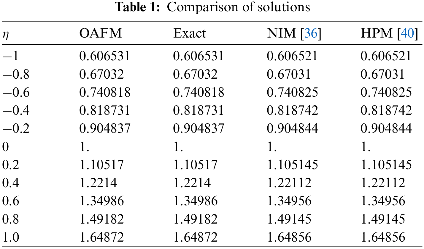
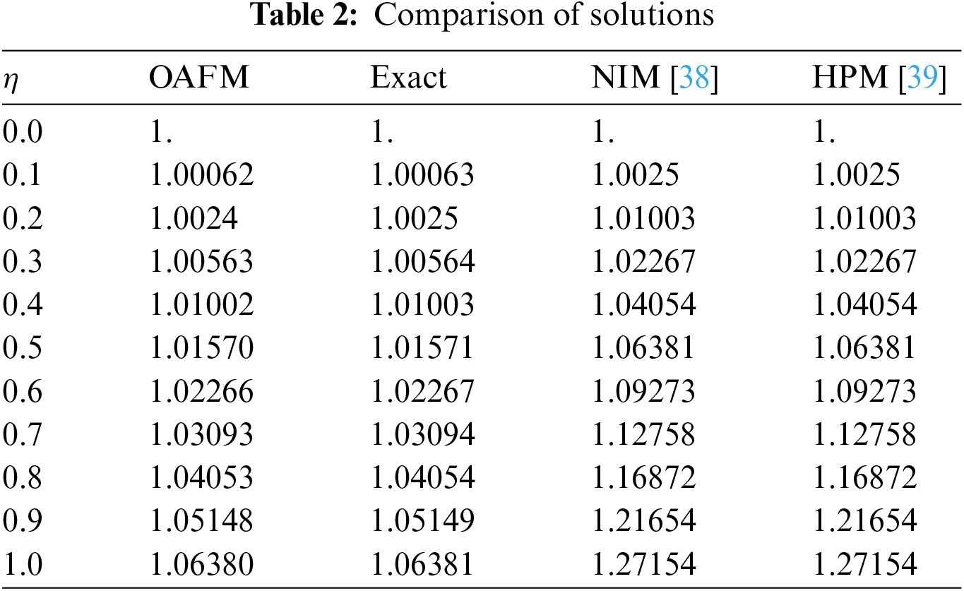
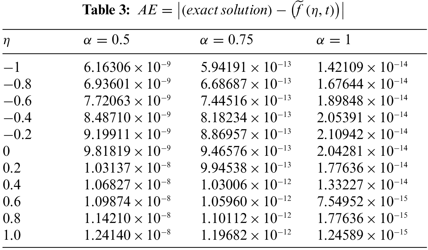
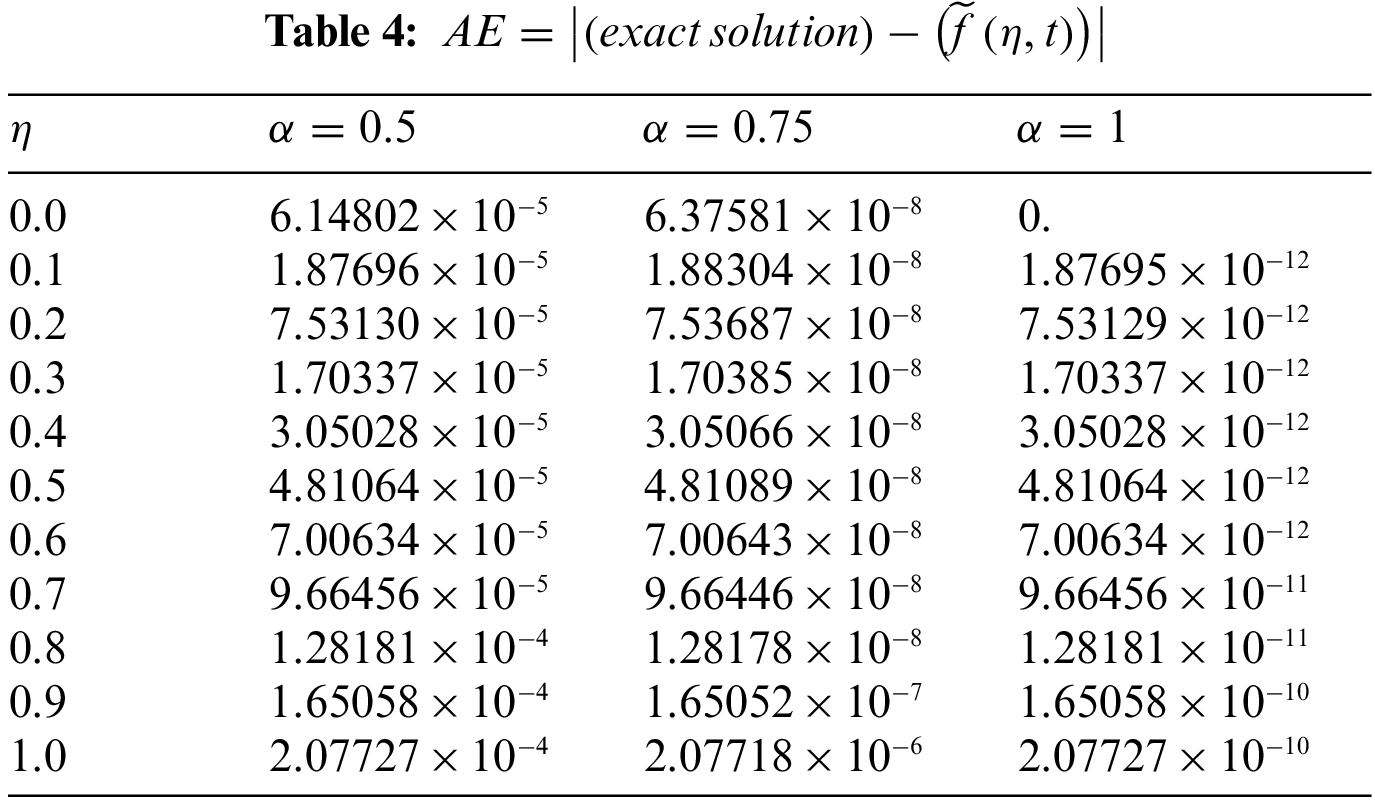
The mathematical theory of FOAFM provides highly accurate solutions for the fractional order Fornberg-Whitham equation as presented in Section 3. We have used Mathematica 11 for our computational work. The results obtained by FOAFM are compared with other methods available in the literature as given in Tables 1 and 2 for both the problems along with the exact solution revealing that FOAFM is valid and more accurate than other analytical methods as FOAFM provides nearly identical results to exact solutions. The absolute errors AEs for both problems are obtained in comparison with exact solutions for different values of fractional order α as given in Tables 3 and 4. It is clear from Tables 3 and 4 that when the value α approaches to unity, then FOAFM solution rapidly converges to exact a solution which again validates our method. The optimal constants for the problem 1 is achieved by using the method of least square and is given as G1 = −5.847118213776651, G2 = −14.401838452215966, G3 = 12.988279917065954, G4 = 6.390562426483602, whereas the optimal constants of the problem 2 are again achieved by the method of least square and are given as C1 = −0.176020345315655812, C2 = −0.04833000998550175, C3 = −1.0800781345410362, C4 = 0.17868188928874937.

The solution is again validated by comparing the solutions with exact solutions in 3D and 2D forms for problems 1–2 as given in Figs. 1–3 and 4–6. The residual plots in 3D and 2D form are given in Figs. 7, 8, 9 and 10 for problems 1 and 2, respectively, while the variation of fractional order α is checked for accuracy in comparison with the exact solution for both the problems in Figs. 11 and 12 consecutively. From Tables 3 and 4 and Figs. 11 and 12, it is evident that when the value of α is closer to 1, then the absolute error decreases and α=1 when used in the FOAFM. We get the closest result to the exact solution validating the accuracy of our method.

Figure 1: 3D plot of f~(η,t)

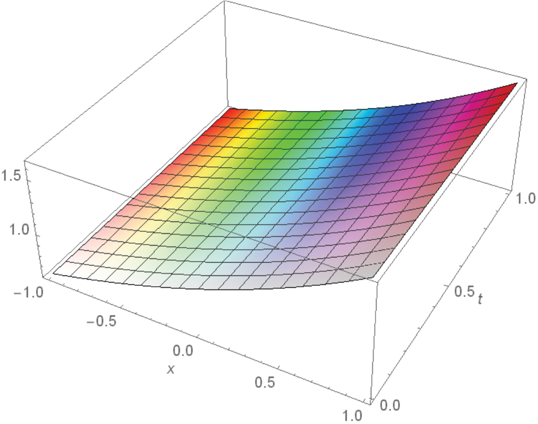
Figure 2: 3D exact solution of f(η,t)

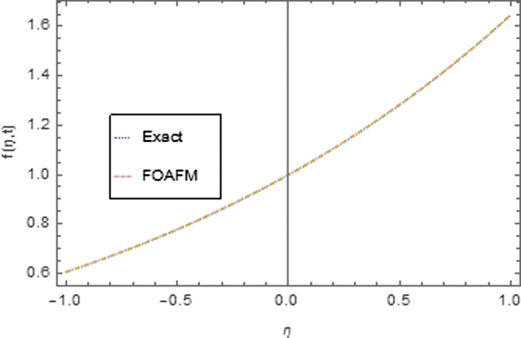
Figure 3: 2D plot of comparison of exact and FOAFM solutions

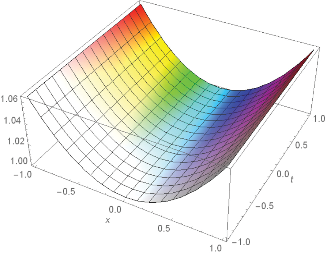
Figure 4: 3D plot of f~(η,t)

Figure 5: 3D exact solution of f(η,t)

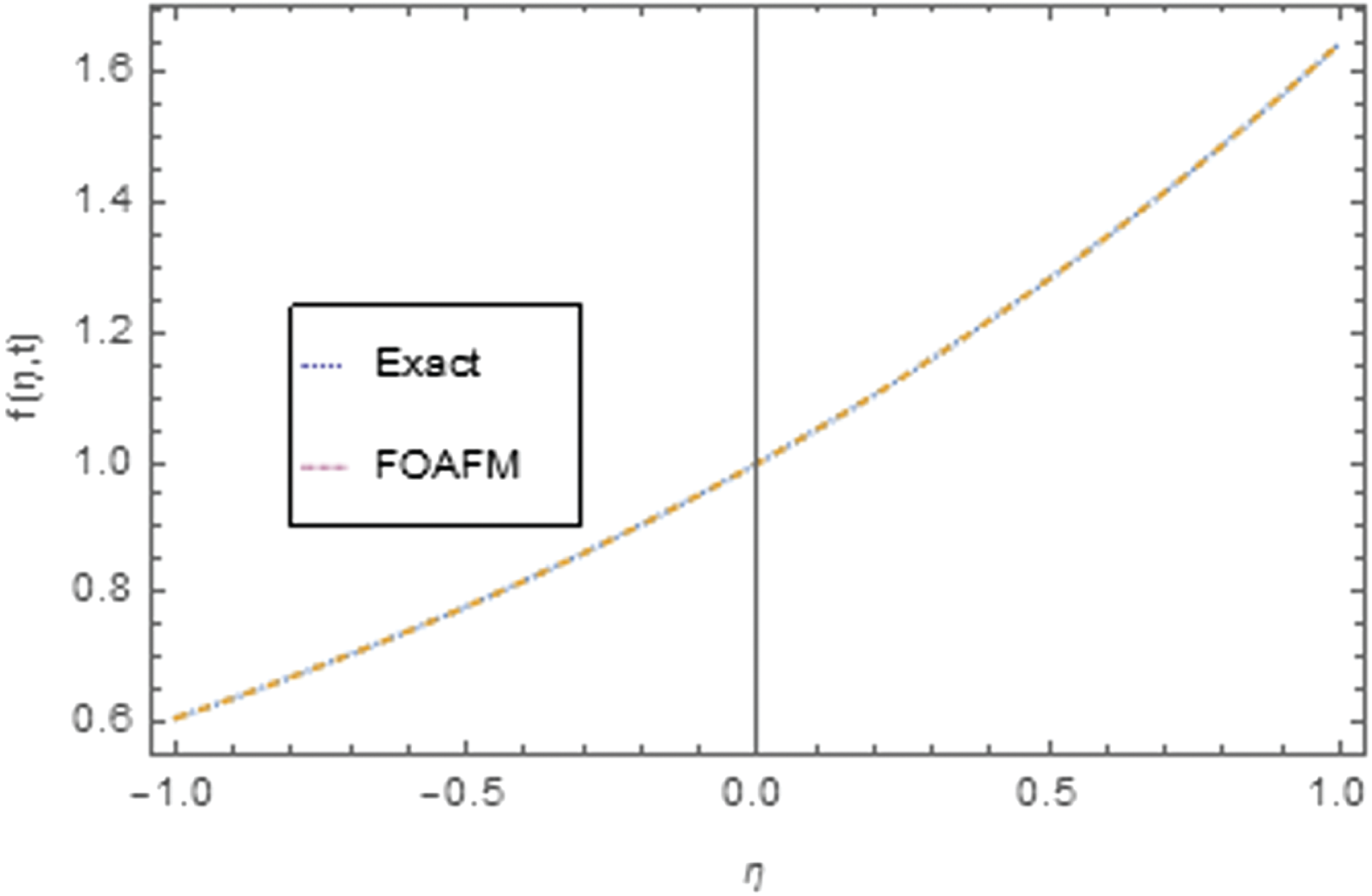
Figure 6: 2D plot of comparison of exact and FOAFM solutions

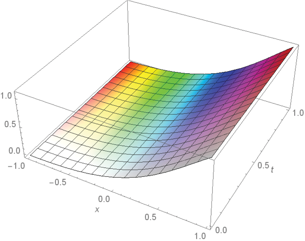
Figure 7: 3D plot of residual

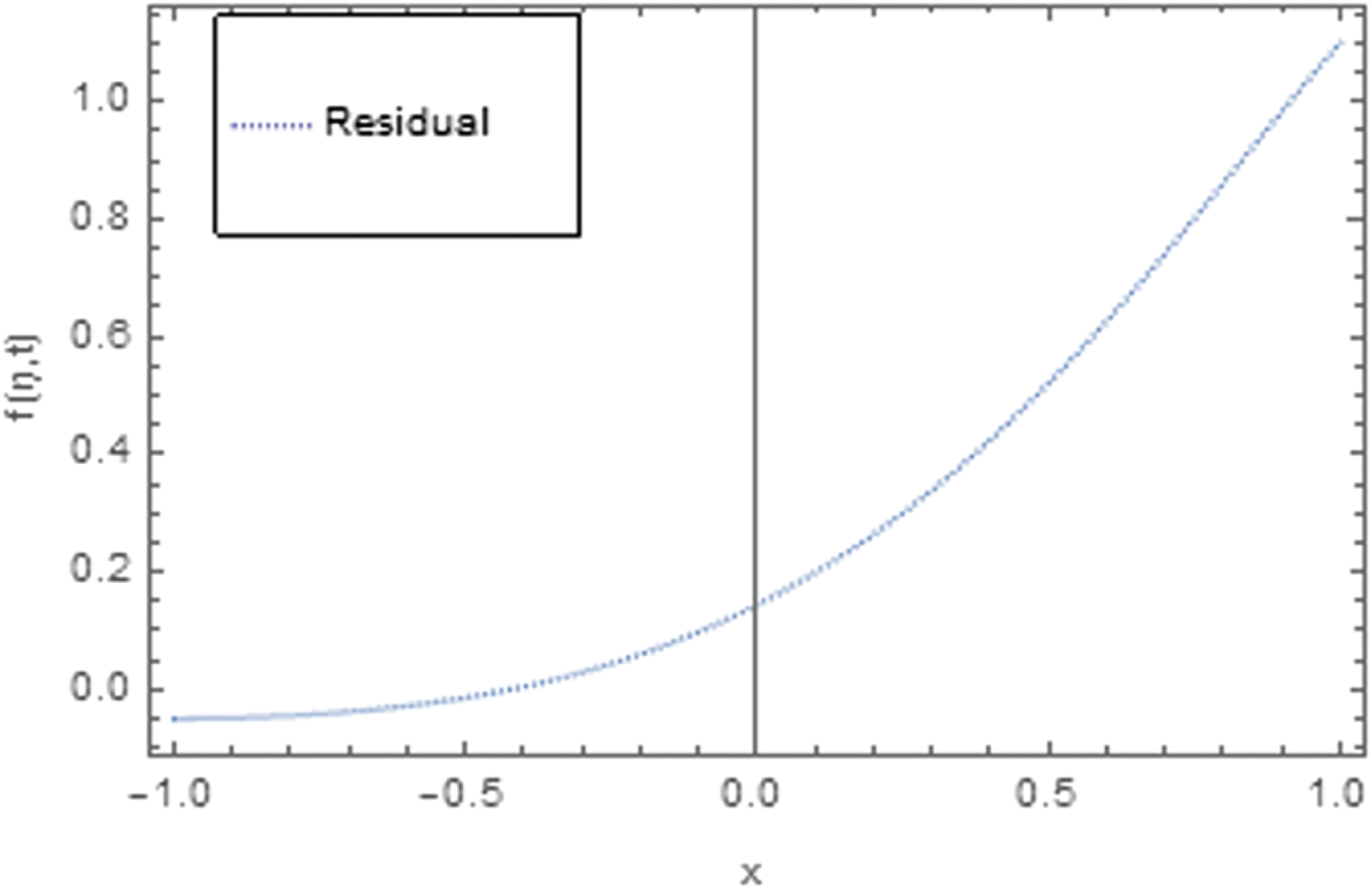
Figure 8: 2D plot of residual

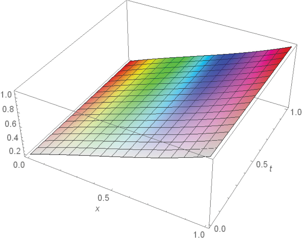
Figure 9: 3D plot of residual

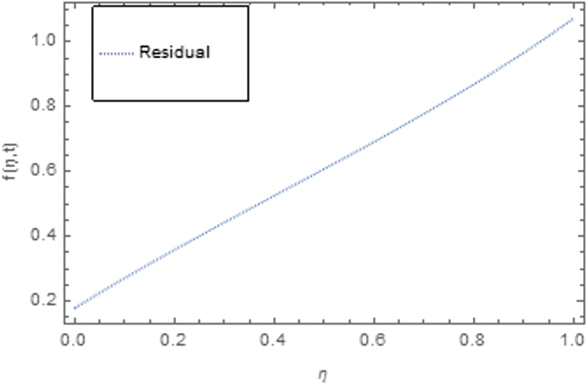
Figure 10: 2D plot of residual

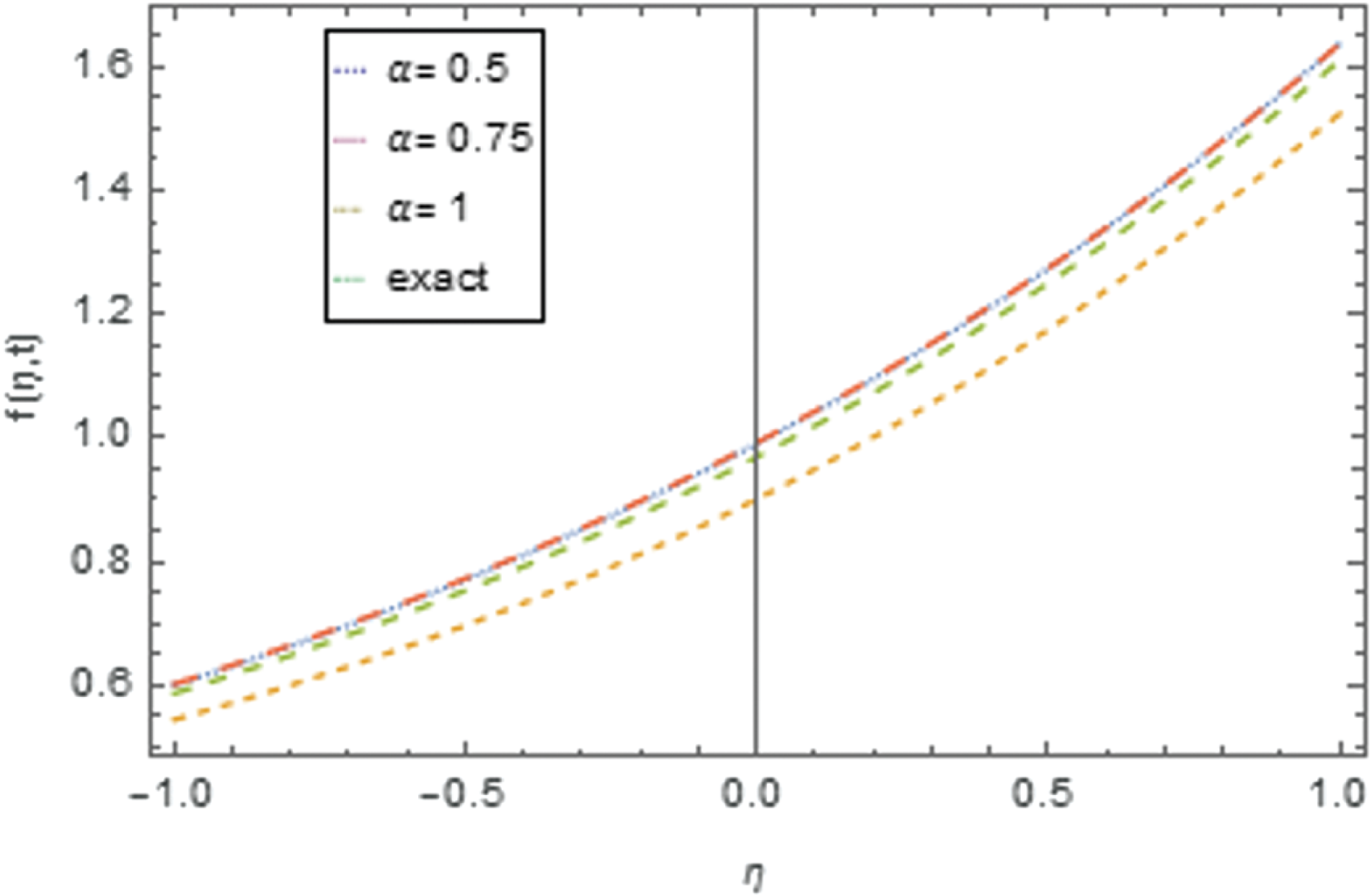
Figure 11: 2D plot of approximate solution for α

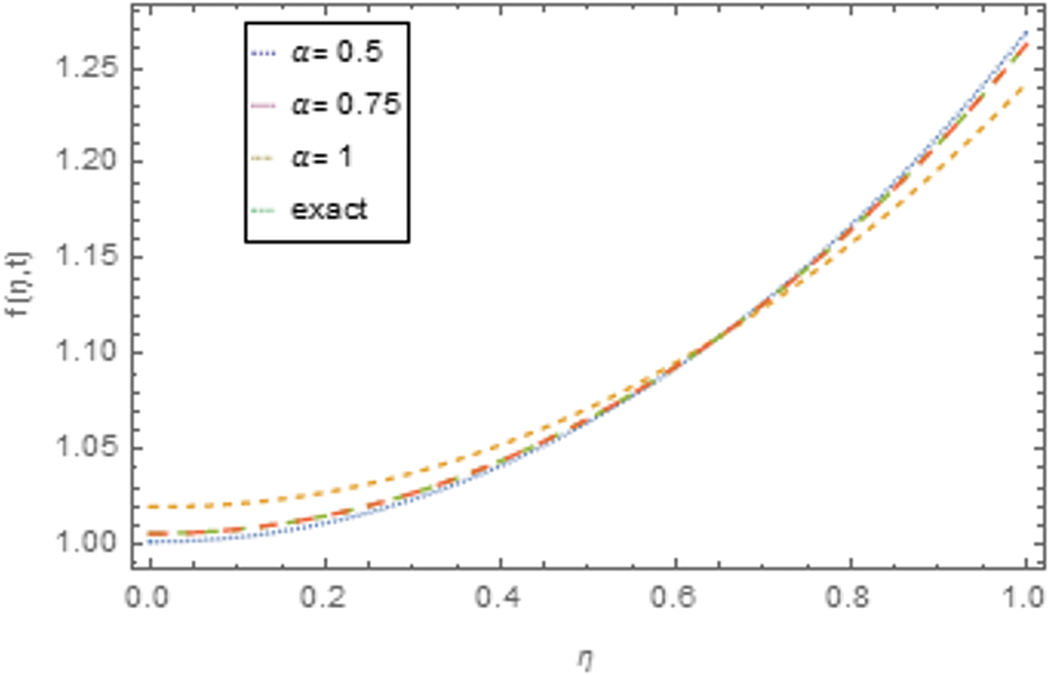
Figure 12: 2D plot of approximate solution for α

6  Conclusion

In this study, a new analytical method is suggested for the solution of the Fornberg-Whitham equation. We obtained the first order series solution for the Fornberg-Whitham equation and achieved the first-order solution with high accuracy. For the accuracy and validity of our method, we compared the FOAFM results with the results available in the literature and the exact results. From the comparison, it is concluded that the suggested method is very accurate and good agreement of our results with the numerical results proves the validity of our method. FOAFM is simply applicable to linear and nonlinear initial and boundary value problems. In comparison with other analytical methods, FOAFM is very easy in applicability and provides us with good results for more complex nonlinear initial/boundary value problems. FOAFM contains the optimal auxiliary constants through which we can control the convergence as FOAFM contains the auxiliary functions D1,D2,D3… in which the optimal constants G1,G2,… and the control convergence parameters exist to play an important role in getting the convergent solution that is obtained rigorously. The computational work in FOAFM is less when compared to other methods and even a low specification computer can do the computational work easily. The less computational work and rapid convergent solution at the first iteration enable us to implement this efficient method in our future work for more complex models arising from real-world problems. The numerical method required maximum space and time as compared to FOAFM which is a short method and very rapidly convergent. Numerical methods are required to have large computational work and require the latest computer for computational work.

Funding Statement: The authors received no specific funding for this study.

Conflicts of Interest: The authors declare that they have no conflicts of interest to report regarding the present study.

References

1. Fellah, Z. E. A., Depollier, C., Fellah, M. (2002). Application of fractional calculus to the sound waves propagation in rigid porous materials: Validation via ultrasonic measurements. Acta Acustica United with Acustica, 88(1), 34–39. [Google Scholar]
2. Sebaa, N., Fellah, Z. E. A., Lauriks, W., Depollier, C. (2006). Application of fractional calculus to ultrasonic wave propagation in human cancellous bone. Signal Processing, 86(10), 2668–2677. DOI 10.1016/j.sigpro.2006.02.015. [Google Scholar] [CrossRef]
3. Meral, F. C., Royston, T. J., Magin, R. (2010). Fractional calculus in viscoelasticity: An experimental study. Communications in Nonlinear Science and Numerical Simulation, 15(4), 939–945. DOI 10.1016/j.cnsns.2009.05.004. [Google Scholar] [CrossRef]
4. Suárez, J. I., Vinagre, B. M., Calderón, A. J., Monje, C. A., Chen, Y. Q. (2003). Using fractional calculus for lateral and longitudinal control of autonomous vehicles. International Conference on Computer Aided Systems Theory, pp. 337–348. Berlin, Heidelberg, Springer. [Google Scholar]
5. Oldham, K. B., Spanier, J. (1974). The fractional calculus. New York: Academic Press. [Google Scholar]
6. Meerschaert, M. M., Scheffler, H. P., Tadjeran, C. (2006). Finite difference methods for two-dimensional fractional dispersion equation. Journal of Computational Physics, 211(1), 249–261. DOI 10.1016/j.jcp.2005.05.017. [Google Scholar] [CrossRef]
7. Metzler, R., Klafter, J. (2004). The restaurant at the end of the random walk: Recent developments in the description of anomalous transport by fractional dynamics. Journal of Physics A: Mathematical and General, 37(31), R161. DOI 10.1088/0305-4470/37/31/R01. [Google Scholar] [CrossRef]
8. Podlubny, I. (1999). Fractional differential equations. New York, NY, USA: Academic Press. [Google Scholar]
9. Schneider, W. R., Wyss, W. (1989). Fractional diffusion and wave equations. Journal of Mathematical Physics, 30(1), 134–144. DOI 10.1063/1.528578. [Google Scholar] [CrossRef]
10. Torrisi, M., Tracina, R., Valenti, A. (1996). A group analysis approach for a nonlinear differential system arising in diffusion phenomena. Journal of Mathematical Physics, 37(9), 4758–4767. DOI 10.1063/1.531634. [Google Scholar] [CrossRef]
11. Drzain, P. G., Johnson, R. S. (1989). An introduction discussion the theory of solution and its diverse applications. Cambridge University Press. [Google Scholar]
12. Abdel-Hamid, B. (2000). Exact solutions of some nonlinear evolution equations using symbolic computations. Computers & Mathematics with Applications, 40(2–3), 291–302. DOI 10.1016/S0898-1221(00)00161-9. [Google Scholar] [CrossRef]
13. Bluman, G., Kumei, S. (1980). On the remarkable nonlinear diffusion equation (∂/∂x)[a (u+b)−2 (∂u/∂x)]−(∂u/∂t)=0. Journal of Mathematical Physics, 21(5), 1019–1023. DOI 10.1063/1.524550. [Google Scholar] [CrossRef]
14. Chun, C. (2009). Fourier-series-based variational iteration method for a reliable treatment of heat equations with variable coefficients. International Journal of Nonlinear Sciences and Numerical Simulation, 10(11–12), 1383–1388. DOI 10.1515/IJNSNS.2009.10.11-12.1383. [Google Scholar] [CrossRef]
15. Chowdhury, S. H. (2011). A comparison between the modified homotopy perturbation method and adomian decomposition method for solving nonlinear heat transfer equations. Journal of Applied Sciences, 11(7), 1416–1420. DOI 10.3923/jas.2011.1416.1420. [Google Scholar] [CrossRef]
16. Yaghoobi, H., Torabi, M. (2011). The application of differential transformation method to nonlinear equations arising in heat transfer. International Communications in Heat and Mass Transfer, 38(6), 815–820. DOI 10.1016/j.icheatmasstransfer.2011.03.025. [Google Scholar] [CrossRef]
17. Ganji, D. D. (2006). The application of He’s homotopy perturbation method to nonlinear equations arising in heat transfer. Physics Letters A, 355(4–5), 337–341. DOI 10.1016/j.physleta.2006.02.056. [Google Scholar] [CrossRef]
18. Bellman, R. (1964). Perturbation techniques in mathematics, physics, and engineeing. New York: Holt, Rinehart and Winston. [Google Scholar]
19. Cole, J. D. (1968). Perturbation methods in applied mathematics. Waltham, MA: Blaisedell. [Google Scholar]
20. O’Malley, R. E. (1974). Introduction to singular perturbation. New York: Academic Press. [Google Scholar]
21. Liao, S. J. (1992). The proposed homotopy analysis technique for the solution of nonlinear problems (Doctoral Dissertation, Ph.D. Thesis). Shanghai Jiao Tong University, China. [Google Scholar]
22. Marinca, V., Herişanu, N., Nemeş, I. (2008). Optimal homotopy asymptotic method with application to thin film flow. Open Physics, 6(3), 648–653. DOI 10.2478/s11534-008-0061-x. [Google Scholar] [CrossRef]
23. Herişanu, N., Marinca, V. (2010). Explicit analytical approximation to large-amplitude non-linear oscillations of a uniform cantilever beam carrying an intermediate lumped mass and rotary inertia. Meccanica, 45(6), 847–855. DOI 10.1007/s11012-010-9293-0. [Google Scholar] [CrossRef]
24. Marinca, V., Herişanu, N., Bota, C., Marinca, B. (2009). An optimal homotopy asymptotic method applied to the steady flow of a fourth-grade fluid past a porous plate. Applied Mathematics Letters, 22(2), 245–251. DOI 10.1016/j.aml.2008.03.019. [Google Scholar] [CrossRef]
25. Herişanu, N., Marinca, V., Dordea, T., Madescu, G. (2008). A new analytical approach to nonlinear vibration of an electrical machine. Proceedings of the Romanian Academy, Series A. Mathematics, Physics, Technical Sciences, Information Science, 9(3), 229–236. [Google Scholar]
26. Marinca, V., Herişanu, N. (2010). Determination of periodic solutions for the motion of a particle on a rotating parabola by means of the optimal homotopy asymptotic method. Journal of Sound and Vibration, 329(9), 1450–1459. DOI 10.1016/j.jsv.2009.11.005. [Google Scholar] [CrossRef]
27. Ullah, H., Islam, S., Idrees, M., Fiza, M., Haq, Z. M. (2014). An extension of the optimal homotopy asymptotic method to coupled schrödinger-KdV equation. International Journal of Differential Equations, 2014, 1–11. DOI 10.1155/2014/106934. [Google Scholar] [CrossRef]
28. Ullah, H., Islam, S., Idrees, M., Arif, M. (2013). Solution of boundary layer problems with heat transfer by optimal homotopy asymptotic method. Abstract and Applied Analysis, 2013, 324869. DOI 10.1155/2013/324869. [Google Scholar] [CrossRef]
29. Ullah, H., Islam, S., Idrees, M., Fiza, M. (2013). Application of optimal homotopy asymptotic method to doubly wave solutions of the coupled Drinfel’d-Sokolov-Wilson equations. Mathematical Problem in Engineering, 2013, 1–8, 362816. [Google Scholar]
30. Ullah, H., Islam, S., Sharidan, S., Khan, I., Fiza, M. (2015). Formulation and application of optimal homotopy asymptotic method for coupled differential difference equations. PLoS One. DOI 10.137/journal.pone.0120127. [Google Scholar] [CrossRef]
31. Ullah, H., Islam, S., Dennis, L. C. C., Abdelhameed, T. N., Khan, I. et al. (2015). Approximate solution of two-dimensional nonlinear wave equation by optimal homotopy asymptotic method. Mathematical Problems in Engineering, 2015, 380104. DOI 10.1155/2015/380104. [Google Scholar] [CrossRef]
32. Herisanu, N., Marinca, V., Madescu, G., Dragan, F. (2019). Dynamic response of a permanent magnet synchronous generator to a wind gust. Energies, 12, 915. DOI 10.3390/en12050915. [Google Scholar] [CrossRef]
33. Abbasbandy, S. (2007). The application of homotopy analysis method to a generalized hirota-satsuama coupled KdV equations. Physics Letters A, 361, 478–483. DOI 10.1016/j.physleta.2006.09.105. [Google Scholar] [CrossRef]
34. Kumar, D., Singh, J., Baleanu, D. (2018). A new analysis of the fornberg-whitham equation pertaining to a fractional derivative with mittag-leffler-type kernel. The European Physical Journal Plus, 133(2), 1–10. DOI 10.1140/epjp/i2018-11934-y. [Google Scholar] [CrossRef]
35. Lu, J. (2011). An analytical approach to the fornberg–whitham type equations by using the variational iteration method. Computers & Mathematics with Applications, 61(8), 2010–2013. DOI 10.1016/j.camwa.2010.08.052. [Google Scholar] [CrossRef]
36. Hashemi, M. S., Haji-Badali, A., Vafadar, P. (2014). Group invariant solutions and conservation laws of the fornberg–whitham equation. Zeitschrift für Naturforschung A, 69(8–9), 489–496. DOI 10.5560/zna.2014-0037. [Google Scholar] [CrossRef]
37. Ramadan, M. A., Al-luhaibi, M. S. (2014). New iterative method for solving the fornberg-whitham equation and comparison with homotopy perturbation transform method. British Journal of Mathematics & Computer Science, 4(9), 1213–1227. [Google Scholar]
38. Merdan, M., Gokdogan, A., Yildirim, A., Mohyud-Din, S. T. (2012). Numerical simulation of fractional fornberg-whitham equation by differential transformation method. Abstract and Applied Analysis, 965367. DOI 10.1155/2012/965367. [Google Scholar] [CrossRef]
39. Wang, K., Liu, S. (2016). Application of new iterative transform method and modified fractional homotopy analysis transform method for fractional fornberg-whitham equation. Journal of Nonlinear Sciences and Applications, 9(5), 2419–2433. DOI 10.22436/jnsa. [Google Scholar] [CrossRef]
40. Abidi, F., Omrani, K. (2011). Numerical solutions for the nonlinear fornberg–whitham equation by he’s methods. International Journal of Modern Physics B, 25(32), 4721–4732. DOI 10.1142/S0217979211059516. [Google Scholar] [CrossRef]
41. Ibrahim, R. W., Ajaj, A. M., Al-Saidi, N. M., Balean, D. (2022). Similarity analytic solutions of a 3D-fractal nanofluid uncoupled system optimized by a fractal symmetric tangent function. Computer Modeling in Engineering & Sciences, 130(1), 221–232. DOI 10.32604/cmes.2022.018348. [Google Scholar] [CrossRef]
42. Liu, C., Kuo, C., Chang, J. (2020). Solving the optimal control problems of nonlinear duffing oscillators by using an iterative shape function method. Computer Modeling in Engineering & Sciences, 122(1), 33–48. DOI 10.32604/cmes.2020.08490. [Google Scholar] [CrossRef]
43. Ghasemi, M. H., Hoseinzadeh, S., Heyns, P. S., Wilke, D. N. (2020). Numerical analysis of non-Fourier heat transfer in a solid cylinder with dual-phase-lag phenomenon. http://hdl.handle.net/2263/73642. [Google Scholar]
44. Gulalai, S. A., Rihan, F. A., Ahmad, S., Rihan, F. A., Ullah, A. et al. (2022). Nonlinear analysis of a nonlinear modified KdV equation under Atangana Baleanu Caputo derivative. AIMS Mathematics, 7(5), 7847–7865. DOI 10.3934/math.2022439. [Google Scholar] [CrossRef]
45. Aljahdaly, N. H., Akgül, A., Shah, R., Mahariq, I., Kafle, J. (2022). A comparative analysis of the fractional-order coupled Korteweg–de Vries equations with the Mittag–Leffler law. Journal of Mathematics, 2022, 8876149. DOI 10.1155/2022/8876149. [Google Scholar] [CrossRef]
46. Wang, K. L. (2022). Novel approach for fractal nonlinear oscillators with discontinuities by Fourier series. Fractals, 30(1), 2250009. DOI 10.1142/S0218348X22500098. [Google Scholar] [CrossRef]
47. Wang, K. (2022). Fractal solitary wave solutions for fractal nonlinear dispersive boussinesq-like models. Fractals, 30(4), 1–8. DOI 10.1142/S0218348X22500839. [Google Scholar] [CrossRef]
48. Gupta, M. D., Chauhan, R. K. (2022). Hardware efficient pseudo-random number generator using chen chaotic system on FPGA. Journal of Circuits, Systems and Computers, 31(3), 2250043. DOI 10.1142/S0218126622500438. [Google Scholar] [CrossRef]
49. Ali, U., Ahmad, H., Baili, J., Botmart, T., Aldahlan, M. A. (2022). Exact analytical wave solutions for space-time variable-order fractional modified equal width equation. Results in Physics, 33, 105216. DOI 10.1016/j.rinp.2022.105216. [Google Scholar] [CrossRef]
50. Mastoi, S., Ganie, A. H., Saeed, A. M., Ali, U., Rajput, U. A. et al. (2022). Numerical solution for two dimensional partialdifferentialequations using SMs method. DOI 10.1515/phys-2022-0015. [Google Scholar] [CrossRef]
51. Naseem, T., Niazi, N., Ayub, M., Sohail, M. (2021). Vectorial reduced DTM for fractional Cauchy riemann system of equations. Computational and Mathematical Methods, 3(6), e1157. [Google Scholar]
52. Shoial, M., Mohyud-Din, S. T. (2012). Reduced DTM for time fractional parabolic PDEs. International Journal of Modern Applied Physics, 1(3), 114–122. [Google Scholar]
53. Wang, Q. L., He, J. H., Li, Z. B. (2012). Fractional model for heat conduction in polar bear hairs. Thermal Science, 16(2), 339–342. DOI 10.2298/TSCI110503070W. [Google Scholar] [CrossRef]
Cite This Article
Copyright © 2023 The Author(s). Published by Tech Science Press.
This work is licensed under a Creative Commons Attribution 4.0 International License , which permits unrestricted use, distribution, and reproduction in any medium, provided the original work is properly cited.
Downloads
Citation Tools