On the Approximation of Fractal-Fractional Differential Equations Using Numerical Inverse Laplace Transform Methods

1  Introduction

Fractional calculus (FC) is the generalization of classical calculus in which we study the differential and integral operators of non integer order. FC can explain numerous real world phenomena with a better memory effect. Initially, fractional calculus was treated as an abstract mathematical idea with almost no application. But within the last few decades, a significant development has been observed in the fields of FC, such as Geo-Hydrology, chaotic processes [1,2], wave propagation, rheology, finance system [3], groundwater flow, and fluid mechanics [4,5], fractional-order dynamical systems in control theory [6], fractional order controller [7], fractional Brownian motion [8], generalized Mittag-Leffler function [9] etc. Until now, various operators of arbitrary order have been introduced in which the two most commonly used with singular kernels are Riemann-Liouville (RL) and Caputo. Similarly, the two famous fractional derivatives with non singular kernels which have been used in literature are the Caputo-Fabrizio (CF) and Atangana-Baleanu (AB) [1,10]. Applications of these fractional derivatives with non singular kernels have been investigated by many researchers in various fields of science and engineering. Some of the reported work is discussed here. For instance, Wang et al. [11] studied fractional Fredholm integro differential equation with AB derivative. Liu et al. [12] investigated Riccati differential equation with AB derivative. Qiang et al. [13] studied Volterra integro differential equation with AB derivative. Gorenflo et al. [14] derived some results for Mittag-Leffler function and related applications. Yavuz et al. [15] investigated a fractional predator-prey model. Sulaiman et al. [16] established some numerical results for fractional coupled viscous Burger’s equation involving Mittag-Leffler kernel.

In literature, numerous methods have been proposed for the analytical and numerical solutions of problems from FC, such as the sinc-collocation method [17], Taylor collocation method [18], Adomian decomposition method [19], variation iteration method [20], RBFs method [21,22], operation matrix method [5], finite difference method [23], etc.

Recently, in [1], the author developed a new idea of fractal-fractional derivative. Fractal-fractional derivative is very suitable in many situations in dealing with real world complex phenomena. This operator has two orders, one is the fractional order and the second is fractal dimension. As compared to other fractional order operators, fractal-fractional derivative is a powerful tool to describe the complex geometry more precisely and efficiently. Usually for the description of irregular and complex geometry fractal-fractional derivative has been used as a powerful tool. The said irregular or complex geometry could not be described by the Caputo fractional derivatives [24,25]. Fractal-fractional operators have not yet been studied extensively. However, few but valuable research articles are available related to the study of fractal fractional differential operators. For instance, authors [26] have developed a numerical method for the numerical solutions of differential equations of fractal-fractional order. In [27], authors have investigated the advection dispersion model. Atangana et al. [25] have derived the exact solution of some important fractal-fractional differential equations. They have also studied the numerical solution for nonlinear cases. Owolabi et al. [28] have developed numerical methods for fractal-fractional Scnakenberg reaction diffusion system. The authors in [5] have proposed an efficient operation matrix method for solving fractal-fractional differential equations. Other valuable work on fractal-fractional differential operators can be found in [29–31] and references therein. But most of these methods are based on the finite difference method for temporal discretization, and they encounter an increase of computing cost with advancing time and thus these methods have low efficiency in the simulation of the long time history of fractional differential equations.

In order to overcome the drawback of the finite difference method for temporal discretization, in this work, we propose a method based on Laplace transform (LT) and numerical inverse Laplace transform (NILT) method. The main idea of the proposed work is to use the LT to reduce the time dependent problem in Caputo sense to an equivalent time independent problem and then solve it in the LT space. Further, a solution of the considered original problem is obtained using NILT. The purpose of using the LT and NILT instead of step-by-step finite difference method for temporal discretization is to avoid the calculation of costly convolution integral in fractal-fractional derivative approximation, and avoid the time stepping technique and the severe stability restrictions in time. In this article, we have utilized three NILT methods: the Talbot’s method, the Euler’s method, and the Stehfest’s method.

The rest of the paper is organized as: in Section 1, some important definitions are given. In Section 2, the methodology of the proposed numerical scheme is described. In Section 3, the numerical examples are given.

1.1 Preliminaries

This section is devoted to some basic definitions from fractional calculus.

Definition 1.1. If G(t) is continuous on (a,b), and G(t) is fractal-differentiable in (a,b) with order β, then the fractal-fractional derivative of G(t) of order α in RL sense is defined in [25] as

1.   with power law kernel

aFFPDtα,βG(t)=1Γ(1−α)ddtβ∫atG(ϑ)(t−ϑ)−αdϑ,(1)

where

dG(ϑ)dϑβ=limt→ϑG(t)−G(ϑ)tβ−ϑβ.(2)

2.   With exponential decay kernel

aFFEDtα,βG(t)=M(α)1−αddtβ∫atG(ϑ)exp(−α1−α(t−ϑ))dϑ,0<α,β≤1.(3)

3.   With generalized Mittag-Leffler (ML) kernel

aFFMDtα,βG(t)=AB(α)1−αddtβ∫atG(ϑ)Eα(−α1−α(t−ϑ)α)dϑ,0<α,β≤1,(4)

where

AB(α)=1−α+αΓ(α).

Definition 1.2. Let G(t) be piecewise continuous function defined for t>0. The LT of G(t) is defined in [25] as

L{G(t)}=G^(z)=∫0∞exp(−zt)G(t)dt.(5)

The three famous derivatives Caputo, CF and AB satisfy the following relations [25]:

0CDtαG(t)=dG(t)dtt−αΓ(1−α).(6)

0CFDtαG(t)=dG(t)dtM(α)1−αexp[−α1−αt].(7)

0ABCDtαG(t)=dG(t)dtAB(α)1−αEα[−α1−αtα].(8)

The LT of these derivatives is given as

L{0CDtαG(t)}=zαL{G(t)}−G(0)z(α−1),(9)

L{0CFDtαG(t)}=−[zL{G(t)}−G(0)]M(α)zα−z−α(10)

and

L{0ABCDtαG(t)}=[zL{G(t)}−G(0)]AB(α)zα−1zα(1−α)+α.(11)

2  Proposed Method

In this section, we propose our numerical method for the approximation of the solution fractal-fractional differential equations with different kernels.

2.1 Power Law Kernel

A power law is a functional relationship between two quantities, where a relative change in one quantity results in a proportional relative change in the other quantity. Power law kernels have significant applications in mathematical modeling of various real world problems. For instance, those problems are related to machines learning, where power law kernels play central role in modeling the process. Furthermore, positive definite kernels are considered as a measure of similarity between points in the kernel based machine learning procedure. Also, theoretic quantities and information based on kernels are usually used in image processing and text mining. The most significant use of power law kernels can be found in the probability distribution theory. Besides, from the mentioned fields, the important applications of the said kernels can be studied in mathematical modeling of various process of cosmology, physics and astronomy as well as in biology. Here, we consider a differential equation with power law kernel of the form [25]

0FFPDtα,βG(t)=Q(t),(12)

which implies

1Γ(1−α)ddtβ∫0tG(ϑ)(t−ϑ)−αdϑ=Q(t),(13)

then

1Γ(1−α)1βtβ−1ddt∫0tG(ϑ)(t−ϑ)−αdϑ=Q(t),(14)

then

1Γ(1−α)ddt∫0tG(ϑ)(t−ϑ)−αdϑ=βtβ−1Q(t),(15)

then, we get

0RLDtαG(t)=βtβ−1Q(t).(16)

Using the relation between the Caputo and RL derivatives, (16) can be written as

0CDtαG(t)=βtβ−1Q(t)−G(0)Γ(1−α)t−α.(17)

Now we take LT of both side of given equation as

L{0CDtαG(t)}=L{βtβ−1Q(t)−G(0)Γ(1−α)t−α},zαL{G(t)}−G(0)zα−1=L{βtβ−1Q(t)}−L{G(0)Γ(1−α)t−α},

which implies

zαL{G(t)}=H^(z),

where

H^(z)=L{βtβ−1Q(t)},

and

L{G(0)Γ(1−α)t−α}=G(0)zα−1.

Simplifying, we get

G^(z)=L{G(t)}=z−αH^(z).(18)

Now the inverse LT of (18) gives

G(t)=L−1{G^(z)}=L−1{z−αH^(z)}.(19)

2.2 Exponential Decay Kernel

We consider a differential equation with exponential decay kernel [25] as

0FFEDtα,βG(t)=Q(t),(20)

which implies

M(α)(1−α)ddtβ∫0tG(ϑ)exp[−α1−α(t−ϑ)]dϑ=Q(t),(21)

then

M(α)(1−α)1βtβ−1ddt∫0tG(ϑ)exp[−α1−α(t−ϑ)]dϑ=Q(t),(22)

then

M(α)(1−α)ddt∫0tG(ϑ)exp[−α1−α(t−ϑ)]dϑ=βtβ−1Q(t),(23)

then, we get

0CFRDtαG(t)=βtβ−1Q(t).(24)

Using the relation between the CF and RL derivatives, (24) can be written as

0CFDtαG(t)=βtβ−1Q(t)−M(α)(1−α)G(0)exp[−α1−α(t)].(25)

Now we take LT of both side of given equation

L{0CFDtαG(t)}=L{βtβ−1Q(t)−M(α)(1−α)G(0)exp[−α1−α(t)]},−[zL{G(t)}−G(0)]M(α)zα−α−z=L{βtβ−1Q(t)}−L{M(α)(1−α)G(0)exp[−α1−α(t)]},−[zL{G(t)}−G(0)]M(α)zα−α−z=L{βtβ−1Q(t)}−M(α)(1−α)G(0)1α1−α+z,

which implies

−[zL{G(t)}]M(α)zα−α−z=H^(z),

where

H^(z)=L{βtβ−1Q(t)},

simplifying, we get

G^(z)=L{G(t)}=zα−α−z−zM(α)H^(z).(26)

Now the inverse LT of (26) gives

G(t)=L−1{G^(z)}=L−1{zα−α−z−zM(α)H^(z).}(27)

2.3 Generalized Mittag-Leffler (ML) Kernel

We consider a differential equation with generalized ML kernel of the form [25]

0FFMDtα,βG(t)=Q(t),(28)

which implies

AB(α)(1−α)ddtβ∫0tG(ϑ)Eα[−α1−α(t−ϑ)α]dϑ=Q(t),(29)

then

AB(α)(1−α)1βtβ−1ddt∫0tG(ϑ)Eα[−α1−α(t−ϑ)α]dϑ=Q(t),(30)

then

AB(α)(1−α)ddt∫0t⁡G(ϑ)Eα[−α1−α(t−ϑ)α]dϑ=βtβ−1Q(t),(31)

then, we get

0ABRDtαG(t)=βtβ−1Q(t).(32)

Using the relation between the AB and RL derivatives, (32) can be written as

0ABCDtαG(t)=βtβ−1Q(t)−AB(α)(1−α)G(0)Eα[−α1−α(tα)].(33)

Now we take LT of both sides of given equation

L{0ABCDtαG(t)}=L{βtβ−1Q(t)−AB(α)(1−α)G(0)Eα[−α1−α(tα)]}(zL{G(t)}−G(0))AB(α)zα−1(zα(1−α)+α)=L{βtβ−1Q(t)}−L{AB(α)(1−α)G(0)Eα[−α1−α(tα)]}[zL{G(t)}−G(0)]AB(α)zα−1(zα(1−α)+α)=L{βtβ−1Q(t)}−AB(α)(1−α)G(0)zα−1α1−α+zα

which implies

[zL{G(t)}]AB(α)zα−1(zα(1−α)+α)=H^(z),

where

H^(z)=L{βtβ−1Q(t)},

Simplifying, we get

G^(z)=L{G(t)}=(zα(1−α)+α)zαAB(α)H^(z).(34)

Now the inverse LT of (34) gives

G(t)=L−1{G^(z)}=L−1{(zα(1−α)+α)zαAB(α)H^(z)}.(35)

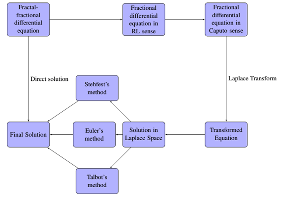
Now we need to approximate the inverse LT in (19), (27), and (35) numerically. In this work, we have utilized three different approaches for this purpose which are (i) Talbot’s method (ii) Euler’s method (iii) Stehfest’s method. The flowchart of the proposed numerical scheme is shown in Fig. 1.

Figure 1: The flowchart of the proposed numerical scheme

2.4 Talbot’s Method (TM)

Using Talbot’s method, the solution of the given problem is obtained as

G(t)=12πι∫ρ−ι∞ρ+ι∞⁡eztG^(z)dz=12πι∫CeztG^(z)dz,Reρ>ρ0(36)

where ρ0 is the converging abscissa and C is a suitably chosen line which connects ρ−ι∞ and ρ+ι∞, which means that all the singularities of the function G(z) lie to the left of C. Its very difficult to approximate the integral defined in (36) due to the highly oscillatory exponential factor ezt and the slow decaying transform G(z). Talbot has suggested in his article [32] that this issue can be resolved using the contour deformation. Furthermore, he suggested that the deformation be done in such a way that real part of the contour starts and ends in the left complex plane inclosing all the singularities of the transform G^(z). On such contours, the integrand decays rapidly owing to the exponential factor, which makes the integral (36) suitable for approximation using the trapezoidal rule or mid point [32,33]. In this work, we consider a contour of the form [33]:

C:z=z(θ),−π≤θ≤π(37)

where Rez(±π)=−inf, and z(θ) is given as

z(θ)=MTtζ(θ),ζ(θ)=−δ+σθcot(μθ)+γιθ,(38)

where μ,ν,γ are to be chosen by the user, using (38) in (36), we have

G(t)=12πι∫CeztG^(z)dz=12πι∫−ππ⁡ez(θ)tG^(z(θ))z′(θ)dθ.(39)

We approximate the latter integral by the N-panel midpoint rule spacing h=2πMT, which yields

GApp(t)≈1MTι∑k=1MT⁡ez(θk)tG^(z(θk))z′(θk),θk=−π+(k−12)h(40)

2.4.1 Convergence of Talbot’s Method

In the approximation of the integral defined in Eq. (39), the convergence of the proposed numerical scheme is achieved at different rates depending on the the contour of integration C. Also the convergence of the proposed scheme depends on the quadrature step h. In order to have optimal results we need to search for optimal contour of integration, which can be done by using the optimal values of the parameters involved in (38). The authors in [33] have proposed optimal values of the parameters as

δ=0.61220,σ=0.50170,γ=0.26450,andμ=0.64070,

with error estimate as

Errorest=|GApp(t)−G(t)|=0(e−1.3580MT).

2.5 Euler’s Algorithm (EA)

In Euler’s inversion formula, to numerically calculate G(t) for the real value of G(t), we have

GApp(t)=10ME3t∑k=02ME⁡ηkRe(G^(βkt))(41)

where

βk=MEln(10)3+πιk,ηk=(−1)kξk(42)

with ι=−1 and ξ0=12, ξk=1,1≤k≤ME,ξ2ME=12ME′

ξ2ME−k=ξ2ME−k+1+2−ME(MEk),0<K<ME.(43)

2.5.1 Convergence of Euler’s Method

To study the effect of the parameter on numerical accuracy, the authors in [34,35] performed a large number of numerical experiments, and they concluded that “if ζ significant digits are required, then suppose ME=[1.7ζ] positive-integer. Set the precision of the system to ME. Given ME and the precision of the system, calculate ηk and βk defined in (42) and (43). Then, given the transform G^(z) and the argument t, calculate the sum GApp(t) in (41)”.

2.6 Stehfest’s Method (SM)

In Stehfest’s method, the approximate value of G(t) is given as

GApp(t)=ln2t∑i=1MS⁡ωiG^(ln2ti),(44)

where the weights ωi are given by

ωi=(−1)MS2+i∑h=⌊i+12⌋min(i,MS2)⁡hMS2(2h!)(MS2−h)!h!(h−1)!(i−h)!(2h−i)!.(45)

Solving (18) for the corresponding Laplace parameters z=ln2ti,i=1,2,3,…,MS. The solution of the original problem can be obtained using (44).

2.6.1 Convergence of Stehfest’s Method

To study the effect of the parameter on numerical accuracy, the authors in [34,35] performed a large number of numerical experiments, and they concluded that “If ζ significant digits are required, suppose MS=⌈2.2ζ⌉ be a positive integer. Set the system precision at δ=⌈1.1MS⌉. Given MS and the system precision, calculate ωi,1≤i≤2MS, using (45). Then, given the transform G^(z) and the argument t, calculate G(t) in (44).” According to these conclusions, we obtain the following error estimation:

Remark 1.

If the error of input data is 10−(δ+1)≤‖G^(z)−G(t)‖‖G(t)‖≤10−δ with even positive integer MS via δ=⌈1.1MS⌉, then the final error is 10−(ζ+1)≤‖G^(z)−G(t)‖‖G(t)‖≤10−ζ, where MS=⌈2.2ζ⌉. It can be found from Remark 1, that the Stehfest’s method tends to demand highly precise input data G^(z) in order to yield best accuracy in the numerical inverse Laplace transform calculations. For example, if input data G^(z) is single-precision data, namely, δ=7 with MS=8, then ζ=4. If input G^(z) are double-precision data, namely, δ=16 with MS=16, then ζ=7 (see [36]).

3  Applications

In this section, we validate our proposed method using numerical experiments. We consider three different fractal-fractional differential equations first with power law kernel, second with exponential decay kernel and third with generalized Mittag-Leffler kernel. The performance of the proposed numerical scheme is evaluated using two error measures. The maximum absolute error AError and the relative error RError are defined as

AError=max|GApp(t)−G(t)|

and

RError=max|GApp(t)−G(t)G(t)|.

Problem 1.

We consider a linear fractal fractional differential equation of the form

0FFPDtα,βz(t)=t3,(46)

with exact solution

z(t)=βΓ(3+β)t(α+β+2)Γ(α+β+3).(47)

The problem is solved using three NILT schemes. In Table 1, the absolute and relative errors of the problem using the Euler’s method are displayed. Tables 2 and 3 show the results obtained using the Talbot’s and Stehfest’s methods for various values of α and β. Fig. 2 shows the plots of numerical and analytic solutions for various values of α and β using the Talbot’s method. The plot of absolute and relative errors for different values of α and β using Euler’s method is shown in Fig. 3. In Fig. 4, the plots of absolute and relative errors of the problem using Talbot’s method are shown. In Fig. 5, the absolute and relative errors for various values of α and β using Stehfest’s method are shown. Similarly in Fig. 6, a comparison between the absolute errors using the three numerical schemes is presented. It is clear from the figure that the Euler’s and Talbot’s methods performed better than the Stehfest’s method.

Figure 2: The plot shows the numerical (markers) and exact (dashed lines) solutions for various values of α,β using Talbot’s method with MT=24. We can see that the numerical solutions have good approximations to the exact solutions

Figure 3: The plot shows the convergence rate of the relative errors (markers) and absolute errors (dashed lines) vs. time for various values of α,β using Talbot’s method with MT=26

Figure 4: The plot shows the convergence rate of the relative errors (markers) and absolute errors (dashed lines) vs. time for various values of α,β using Euler’s method with ME=32

Figure 5: The plot shows the convergence rate of the relative errors (markers) and absolute errors (dashed lines) vs. time for various values of α,β using Stehfest’s method with MS=18

Figure 6: The plot shows the comparison of the convergence rate of the absolute errors of the three methods, Euler’s method with ME=32, Stehfest’s method with MS=18, and Talbot’s method with MT=28. E=0.1,S=0.1,T=0.1 refers to absolute error of Euler’s, Stehfest’s and Talbot’s method with α=β=0.1 respectively and similarly for others

Problem 2.

We consider a linear fractal fractional differential equation of the form

0FFEDtα,βu(t)=t3(48)

With exact solution

u(t)=βΓ(3+β)M(α)[αtΓ(β+4)+1−αΓ(β+3)]tβ+2(49)

The problem is solved using three NILT schemes. In Table 4, the absolute and relative errors of the problem using the Euler’s method are displayed. Tables 5 and 6 show the results obtained using the Talbot’s and Stehfest’s methods for various values of α and β. Fig. 7 shows the plots of numerical and analytic solutions for various values of α and β using the Talbot’s method. The plot of absolute and relative errors for different values of α and β using Euler’s method is shown in Fig. 8. Fig. 9 shows the plot of absolute and relative errors of the problem using Talbot’s method. In Fig. 10, the absolute and relative errors for various values of α and β using Stehfest’s method are shown. Similarly in Fig. 11, a comparison between the absolute errors using the three schemes is presented. It is clear from the figure that the Euler’s and Talbot’s methods performed better than the Stehfest’s method.

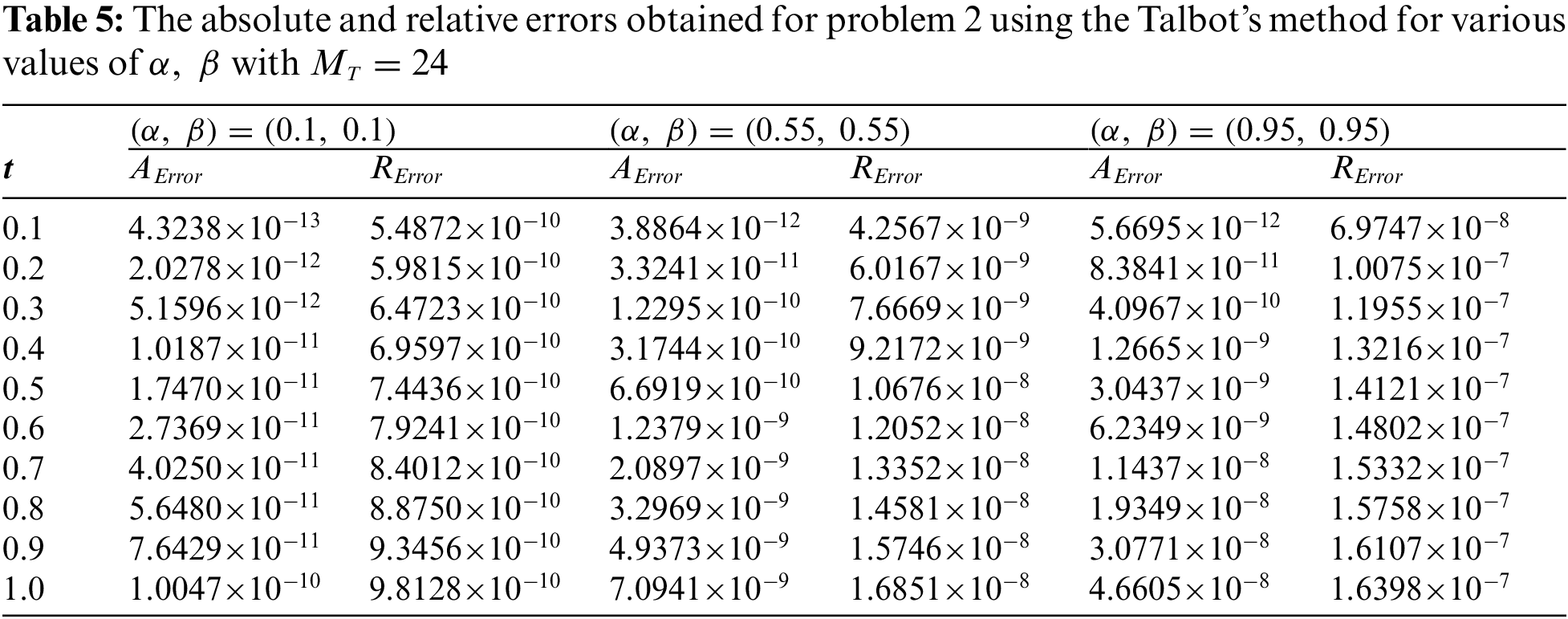
Figure 7: The plot shows the numerical solutions (markers) and exact solutions (dashed lines) for various values of α,β using Euler’s method with ME=34. We can see that the numerical solutions have good approximations to the exact solutions

Figure 8: The plot shows the convergence rate of the relative errors (markers) and absolute errors (dashed lines) vs. time for various values of α,β using Euler’s method with ME=34

Figure 9: The plot shows the convergence rate of the relative errors (markers) and absolute errors (dashed lines) vs. time for various values of α,β using Talbot’s method with MT=26

Figure 10: The plot shows the convergence rate of the relative errors (markers) and absolute errors (dashed lines) vs. time for various values of α,β using Stehfest’s method with MS=24

Figure 11: The plot shows the comparison of the convergence rate of the absolute errors of the three methods Euler method with ME=34, Stehfest’s method with MS=24, and Talbot’s method with MT=26. E=0.1,S=0.1,T=0.1 refers to absolute error of Euler’s, Stehfest’s and Talbot’s method with α=β=0.1 and similarly for others

Problem 3.

We consider a linear fractal fractional differential equation of the form

0FFMDtα,βu(t)=t3,(50)

with exact solution

u(t)=tβ+2βΓ(3+β)AB(α)[1−αΓ(β+3)+αtαΓ(β+α+3)](51)

The problem is solved using three NILT schemes. In Table 7, the absolute and relative errors of the problem using the Euler’s method are displayed. Tables 8 and 9 show the results obtained using the Talbot’s and Stehfest’s methods for various values of α and β. Fig. 12 shows the plots of numerical and analytic solutions for various values of α and β using the Talbot’s method. The plots of absolute and relative errors for various values of α and β using Euler’s method are shown in Fig. 13. Fig. 14 shows the plots of absolute and relative errors of the problem using Talbot’s method. In Fig. 15, the absolute and relative errors for various values of α and β using Stehfest’s method are shown. Similarly in Fig. 16 a comparison between the absolute errors using the three schemes is presented. It is clear from the figure that the Euler’s and Talbot’s methods performed better than the Stehfest’s method.

Figure 12: The plot shows the numerical solutions (markers) and exact solutions (dashed lines) for different values of α,β using Stehfest’s method with ME=26. We can see that the numerical solutions have good approximations to the exact solutions

Figure 13: The plot shows the convergence rate of the relative errors (markers) and absolute errors (dashed lines) vs. time for various values of α,β using Euler’s method with ME=30

Figure 14: The plot shows the convergence rate of the relative errors (markers) and absolute errors (dashed lines) vs. time for various values of α,β using Talbot’s method with MT=22

Figure 15: The plot shows the convergence rate of the relative errors (markers) and absolute errors (dashed lines) vs. time for various values of α,β using Stehfest’s method with MS=20

Figure 16: The plot shows the comparison of the convergence rate of the absolute errors of the three methods Euler method with ME=30, Stehfest’s method with MS=20, and Talbot method with MT=22. E=0.1,S=0.1,T=0.1 refers to absolute error of Euler’s, Stehfest’s and Talbot’s methods with α=β=0.1 and similarly for others

4  Conclusions

New concepts of differentiation and integration have been introduced recently. The new differentiation is a combination of fractal and fractional differentiation. In this paper, we have developed a Laplace transformed method for numerical modeling of fractal-fractional differential equations. In contrast to the standard finite difference method, the proposed method has used the Laplace transform and numerical Laplace inversion to handle the time fractal-fractional derivative. Solving differential equations of fractal-fractional order using time stepping technique may face the problem of time-instability. However, this method avoids the time stepping method and hence the time-instability. We have utilized three Laplace transform inversion methods to evaluate the time domain solution for three fractal-fractional differential equations. In all cases, the inversion results have been proven excellent. All three inversion methods have produced accurate results. From the obtained results, it has been observed that Euler’s and Talbot’s methods are more accurate than Stehfest’s method. Furthermore, it has also observed that using Stehfest’s method, optimal accuracy can be achieved for values of MS around 20 or 22. Hence, the obtained results led us to the conclusion that these methods are excellent alternatives for approximating the solutions of such types of differential equations. It was also found that these inversion methods are applicable to such types of fractal-fractional differential equations. The proposed methods are easy to implement and highly accurate.

Acknowledgement: The authors K. Shah, T. Abdeljawad and B. Abdalla would like to thank Prince Sultan University for the support through the TAS Research Lab.

Funding Statement: The APC of this article is supported by Prince Sultan University.

Conflicts of Interest: The authors declare that they have no conflicts of interest to report regarding the present study.

References

1. Atangana, A. (2017). Fractal-fractional differentiation and integration: Connecting fractal calculus and fractional calculus to predict complex system. Chaos, Solitons & Fractals, 102, 396–406. DOI 10.1016/j.chaos.2017.04.027. [Google Scholar] [CrossRef]
2. Atangana, A., Qureshi, S. (2019). Modeling attractors of chaotic dynamical systems with fractal-fractional operators. Chaos, Solitons & Fractals, 123, 320–337. DOI 10.1016/j.chaos.2019.04.020. [Google Scholar] [CrossRef]
3. Kilbas, A. A., Srivastava, H. M., Trujillo, J. J. (2006). Theory and applications of fractional differential equations. USA: Elsevier Science Inc. [Google Scholar]
4. Podlubny, I. (1998). Fractional differential equations: An introduction to fractional derivatives, fractional differential equations, to methods of their solution and some of their applications. USA: Academic Press. [Google Scholar]
5. Shloof, A. M., Senu, N., Ahmadian, A., Salahshour, S. (2021). An efficient operation matrix method for solving fractal-fractional differential equations with generalized Caputo-type fractional-fractal derivative. Mathematics and Computers in Simulation, 188, 415–435. DOI 10.1016/j.matcom.2021.04.019. [Google Scholar] [CrossRef]
6. Debnath, L. (2003). Recent applications of fractional calculus to science and engineering. International Journal of Mathematics and Mathematical Sciences, 2003(54), 3413–3442. DOI 10.1155/S0161171203301486. [Google Scholar] [CrossRef]
7. Bohannan, G. W. (2008). Analog fractional order controller in temperature and motor control applications. Journal of Vibration and Control, 14(9–10), 1487–1498. DOI 10.1177/1077546307087435. [Google Scholar] [CrossRef]
8. Baillie, R. T. (1996). Long memory processes and fractional integration in econometrics. Journal of Econometrics, 73(1), 5–59. DOI 10.1016/0304-4076(95)01732-1. [Google Scholar] [CrossRef]
9. Kilbas, A. A., Saxena, R. K., Saigo, M. (2004). Generalized Mittag-Leffler function and generalized fractional calculus operators. Integral Transforms and Special Functions, 15(1), 31–49. DOI 10.1080/10652460310001600717. [Google Scholar] [CrossRef]
10. Atangana, A., Baleanu, D. (2016). New fractional derivatives with nonlocal and non-singular kernel: Theory and application to heat transfer model. Thermal Science, 20, 763–769. DOI 10.2298/TSCI160111018A. [Google Scholar] [CrossRef]
11. Wang, J., Kamran, Jamal, A., Li, X. (2021). Numerical solution of fractional-order Fredholm integrodifferential equation in the sense of Atangana-Baleanu derivative. Mathematical Problems in Engineering, 2021, 1–8. DOI 10.1155/2021/3839800. [Google Scholar] [CrossRef]
12. Liu, X., Kamran, Yao, Y. (2020). Numerical approximation of Riccati fractional differential equation in the sense of Caputo-type fractional derivative. Journal of Mathematics, 2020, 1–12. [Google Scholar]
13. Qiang, X., Kamran, Mahboob, A., Chu, Y. M. (2020). Numerical approximation of fractional-order volterra integrodifferential equation. Journal of Function Spaces, 2020, 1–12. DOI 10.1155/2020/8875792. [Google Scholar] [CrossRef]
14. Gorenflo, R., Kilbas, A. A., Mainardi, F., Rogosin, S. V. (2020). Mittag-leffler functions, related topics and applications. New York, NY, USA: Springer. [Google Scholar]
15. Yavuz, M., Sene, N. (2020). Stability analysis and numerical computation of the fractional predator-prey model with the harvesting rate. Fractal and Fractional, 4(3), 1–22. DOI 10.3390/fractalfract4030035. [Google Scholar] [CrossRef]
16. Sulaiman, T. A., Yavuz, M., Bulut, H., Baskonus, H. M. (2019). Investigation of the fractional coupled viscous Burger’s equation involving Mittag-Leffler kernel. Physica A: Statistical Mechanics and its Applications, 527, 121126. DOI 10.1016/j.physa.2019.121126. [Google Scholar] [CrossRef]
17. Alkan, S., Hatipoglu, V. F. (2017). Approximate solutions of Volterra-Fredholm integro-differential equations of fractional order. Tbilisi Mathematical Journal, 10(2), 1–13. [Google Scholar]
18. Öztürk, Y., Anapalı, A., Gülsu, M., Sezer, M. (2013). A collocation method for solving fractional Riccati differential equation. Journal of Applied Mathematics, 5(6), 872–884. [Google Scholar]
19. Rani, D., Mishra, V. (2018). Modification of Laplace adomian decomposition method for solving nonlinear volterra integral and integro-differential equations based on Newton Raphson formula. European Journal of Pure and Applied Mathematics, 11(1), 202–214. DOI 10.29020/nybg.ejpam.v11i1.2645. [Google Scholar] [CrossRef]
20. Ahmad, H., Seadawy, A. R., Khan, T. A. (2020). Study on numerical solution of dispersive water wave phenomena by using a reliable modification of variational iteration algorithm. Mathematics and Computers in Simulation, 177, 13–23. DOI 10.1016/j.matcom.2020.04.005. [Google Scholar] [CrossRef]
21. Li, X., Kamran, Haq, A., Zhang, X. (2020). Numerical solution of the linear time fractional Klein-Gordon equation using transform based localized RBF method and quadrature. AIMS Mathematics, 5(5), 5287–5308. DOI 10.3934/math.2020339. [Google Scholar] [CrossRef]
22. Li, J., Dai, L., Kamran, Nazeer, W. (2020). Numerical solution of multi-term time fractional wave diffusion equation using transform based local meshless method and quadrature. AIMS Mathematics, 5(6), 5813–5839. DOI 10.3934/math.2020373. [Google Scholar] [CrossRef]
23. Jacobs, B. A. (2016). High-order compact finite difference and Laplace transform method for the solution of time-fractional heat equations with dirchlet and Neumann boundary conditions. Numerical Methods for Partial Differential Equations, 32(4), 1184–1199. DOI 10.1002/num.22046. [Google Scholar] [CrossRef]
24. Akgül, A. (2018). A novel method for a fractional derivative with non-local and non-singular kernel. Chaos, Solitons & Fractals, 114, 478–482. DOI 10.1016/j.chaos.2018.07.032. [Google Scholar] [CrossRef]
25. Atangana, A., Akgül, A. (2021). On solutions of fractal fractional differential equations. Discrete & Continuous Dynamical Systems-S, 14(10), 3441–3457. DOI 10.3934/dcdss.2020421. [Google Scholar] [CrossRef]
26. Attia, A., Akgül, A., Seba, D., Nour, A., Asa, J. (2022). A novel method for fractal-fractional differential equations. Alexandria Engineering Journal, 61(12), 9733–9748. DOI 10.1016/j.aej.2022.02.004. [Google Scholar] [CrossRef]
27. Atangana, A., Akgül, A., Owolabi, K. M. (2020). Analysis of fractal fractional differential equations. Alexandria Engineering Journal, 59(3), 1117–1134. DOI 10.1016/j.aej.2020.01.005. [Google Scholar] [CrossRef]
28. Owolabi, K. M., Atangana, A., Akgul, A. (2020). Modelling and analysis of fractal-fractional partial differential equations: Application to reaction-diffusion model. Alexandria Engineering Journal, 59(4), 2477–2490. DOI 10.1016/j.aej.2020.03.022. [Google Scholar] [CrossRef]
29. Arif, M., Kumam, P., Kumam, W., Akgul, A., Sutthibutpong, T. (2021). Analysis of newly developed fractal- fractional derivative with power law kernel for MHD couple stress fluid in channel embedded in a porous medium. Scientific Reports, 11(1), 1–20. [Google Scholar]
30. Abro, K. A., Atangana, A. (2020). Mathematical analysis of memristor through fractal-fractional differential operators: A numerical study. Mathematical Methods in the Applied Sciences, 43(10), 6378–6395. DOI 10.1002/mma.6378. [Google Scholar] [CrossRef]
31. Akgül, A. (2021). Analysis and new applications of fractal fractional differential equations with power law kernel. Discrete & Continuous Dynamical Systems-S, 14(10), 3401–3417. DOI 10.3934/dcdss.2020423. [Google Scholar] [CrossRef]
32. Talbot, A. (1979). The accurate numerical inversion of Laplace transforms. IMA Journal of Applied Mathematics, 23(1), 97–120. DOI 10.1093/imamat/23.1.97. [Google Scholar] [CrossRef]
33. Dingfelder, B., Weideman, J. A. C. (2015). An improved talbot method for numerical Laplace transform inversion. Numerical Algorithms, 68(1), 167–183. DOI 10.1007/s11075-014-9895-z. [Google Scholar] [CrossRef]
34. Abate, J., Valkó, P. P. (2004). Multi-precision laplace transform inversion. International Journal for Numerical Methods in Engineering, 60(5), 979–993. DOI 10.1002/(ISSN)1097-0207. [Google Scholar] [CrossRef]
35. Abate, J., Whitt, W. (2006). A unified framework for numerically inverting Laplace transforms. INFORMS Journal on Computing, 18(4), 408–421. DOI 10.1287/ijoc.1050.0137. [Google Scholar] [CrossRef]
36. Fu, Z. J., Chen, W., Yang, H. T. (2013). Boundary particle method for Laplace transformed time fractional diffusion equations. Journal of Computational Physics, 235, 52–66. DOI 10.1016/j.jcp.2012.10.018. [Google Scholar] [CrossRef]
Cite This Article
Copyright © 2023 The Author(s). Published by Tech Science Press.
This work is licensed under a Creative Commons Attribution 4.0 International License , which permits unrestricted use, distribution, and reproduction in any medium, provided the original work is properly cited.
Downloads
Citation Tools