 Open Access
ARTICLE
Dendritic Cell Algorithm with Grouping Genetic Algorithm for Input Signal Generation
1 School of Computer Science, Wuhan University, Wuhan, 430072, China
2 School of Cyber Science and Engineering, Wuhan University, Wuhan, 430072, China
* Corresponding Author: Yiwen Liang. Email:
(This article belongs to the Special Issue: Swarm Intelligence and Applications in Combinatorial Optimization)
Computer Modeling in Engineering & Sciences 2023, 135(3), 2025-2045. https://doi.org/10.32604/cmes.2023.022864
Received 30 March 2022; Accepted 15 August 2022; Issue published 23 November 2022
Abstract
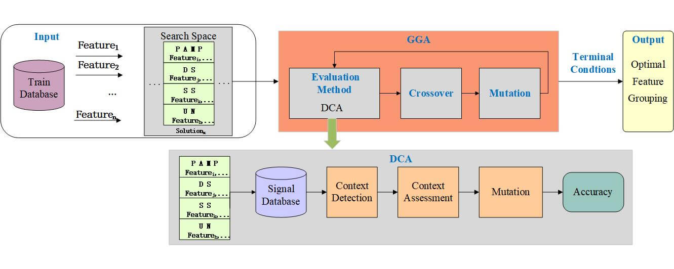
The artificial immune system, an excellent prototype for developing Machine Learning, is inspired by the function of the powerful natural immune system. As one of the prevalent classifiers, the Dendritic Cell Algorithm (DCA) has been widely used to solve binary problems in the real world. The classification of DCA depends on a data pre-processing procedure to generate input signals, where feature selection and signal categorization are the main work. However, the results of these studies also show that the signal generation of DCA is relatively weak, and all of them utilized a filter strategy to remove unimportant attributes. Ignoring filtered features and applying expertise may not produce an optimal classification result. To overcome these limitations, this study models feature selection and signal categorization into feature grouping problems. This study hybridizes Grouping Genetic Algorithm (GGA) with DCA to propose a novel DCA version, GGA-DCA, for accomplishing feature selection and signal categorization in a search process. The GGA-DCA aims to search for the optimal feature grouping scheme without expertise automatically. In this study, the data coding and operators of GGA are redefined for grouping tasks. The experimental results show that the proposed algorithm has significant advantages over the compared DCA expansion algorithms in terms of signal generation.Graphic Abstract
Keywords
The natural immune system assists in recognizing pathogens that can cause destructive infections in individuals and has certain key characteristics: diversity, distributive, dynamic, adaptivity, and robustness [1]. Inspired by its function, several researchers mixed the mechanisms of immunity and computers to propose a collection of bio-inspired algorithms. DCA, one of its prevalent paradigms, is inspired by the functioning of the dendritic cells in the natural immune system [2]. DCA has been widely applied in classification [3,4], anomaly detection [5,6], spam filtering [7], distributed and parallel operations [8], fuzzy clustering, privacy preservation, and earthquake prediction [9]. DCA is designed for low-dimensional space, and the inputs of DCA correspond to three immune signals respectively, named pathogen-associated molecular patterns (PAMP), danger signals (DS), and safe signals (SS) [2]. Generally, the DCA appropriately maps a given problem domain to the input space of DCA in a pre-processing and initialization phase, which is crucial to obtaining reliable results. Recalling from the literature review [10], dimensionality reduction and signal categorization are the main works to generate input signals in the pre-processing and initialization phase. The task of dimensionality reduction is to create a new feature space with low dimensionality. After dimensionality reduction, each feature in the new feature space is assigned to a specific signal category, either PAMP, DS, or SS. Researchers utilized several dimensionality reduction techniques to create a new feature space with low dimensionalities, such as Principal Component Analysis (PCA) [11], Correlation Coefficient (CC) [12], Information Gain (IG) [12], Rough Set Theory (RST) [13–15], and Fuzzy Rough Set Theory (FRST) [16,17]. These approaches filtered weakly important or unimportant features and selected the most important features with their data-intrinsic methods. However, it is essential to realize that relevance/importance according to those definitions does not imply membership in the optimal feature subset, and irrelevance does not mean that a feature can not be in the optimal feature subset [18]. In addition, machine learning algorithms, such as K-Nearest Neighbors (KNN) [19] and Support Vector Machine (SVM) [20], are employed for input signal generation. Moreover, Zhou et al. [1] utilized numerical differential to extract features based on the data changes of the selected features. Among these methods, some approaches may not generate the optimal feature subset due to ignoring the effects of those filtered features; moreover, some approaches are unable to describe the relationship between the attributes and signal categorization.
After dimensionality reduction, each feature in the new feature space is assigned to a specific signal category, either PAMP, DS, or SS. For signal categorization, researchers focus on building a mapping between attributes and signal categories. An appropriate mapping relationship helps achieve good classification results. Several approaches assign a specific signal category to each selected feature by generating a mapping relationship grounded on expert knowledge; others perform signal categorization based on the importance ranking of selected features and the importance ranking of signals. However, the mapping with specialist knowledge may not assign attributes to the most suitable signal categories. In addition, the mapping based on attributes ranking could not be considered a coherent and consistent categorization procedure, leading to unsatisfactory classification results. Several researchers employed a search strategy to find an optimal mapping to overcome the problem. But the approaches with search strategy exclude the filtered features from the original feature space and ignore the effects of the filtered features on the performance of DCA. Among these methods, some algorithms rely on expertise; some establish a mapping in terms of the relationship between the importance of attributes and signals; others ignore the effects of the filtered features, resulting in unsatisfactory classification results.
Therefore, this research is motivated by the following question: how to automatically perform the feature selection and signal categorization, considering all features’ effects for DCA? Inspired by the research about combinatorial optimization, this study transforms feature selection and signal categorization into a feature grouping problem. The features from the original data set are divided into four groups:
This paper is structured as follows: Section 2 describes related work; the DCA is introduced in Section 3; The novel model, GGA-DCA, is proposed in Section 4; our following experiment setup, results and analysis are described in Section 5; conclusions and future work are shown in Section 6.
The classical DCA is proposed by Greensmith et al. [2] which mimics the functioning of the dendritic cells in the natural immune system. The classical DCA relies on artificial experience for feature selection and signal categorization. Aiming to overcome the limitations of the manual method, PCA, CC, IG, RST, and FRST are applied to perform those works.
Gu et al. [11] employed PCA as a feature extraction technique to project the original data onto the principal subspace. They constructed a low-dimensional space with new features. Due to destroying the underlying meaning behind the features present, feature extraction techniques are undesirable for DCA. In [12], the CC and IG were adopted to measure the relevance between attributes and the class. The features whose relevance degree exceeds a certain threshold were selected. Chelly et al. [13–15] proposed RST-DCA and RC-DCA by hybridizing the RST and DCA. RST-DCA and RC-DCA measured the importance of a feature by computing the difference between the positive region of an original data set and the positive region of the data set without this feature. Based on the importance of features, REDUCTs and CORE are achieved as candidates of optimal feature subset. Due to the expensive costs of calculating REDUCTs and CORE, QR-DCA [15] introduced the QuickReduct algorithm to generate only one REDUCT. RST-DCA assigned only one attribute randomly from a REDUCT to both PAMP and SS based on expert knowledge, as well as combined the rest features of REDUCT to represent DS. RC-DCA and QR-DCA assigned attributes of the CORE to both PAMP and SS based on expert knowledge, as well as combined the rest features of REDUCT to represent DS.
The hybrid DCA versions with RST rely upon crisp data sets. Chelly et al. [16,17] integrated FRST with DCA to provide feature reduction for both crisp and real-value attributed datasets. In [17], a greed search and fuzzy lower approximation were applied to obtain a new DCA version, FLA-DCA. The FLA-DCA calculates a feature reduction with the same fuzzy-rough dependency degree as the entire database. In [16], fuzzy boundary region-based DCA (FBR-DCA) was proposed subsequently. The FBR-DCA utilized a greed search and the fuzzy boundary region to find a feature reduction with the minimal uncertainty degree based on fuzzy rough set theory. FLA-DCA selected the feature with the most significant fuzzy-rough dependency degree to form the SS, the second attribute to form PAMP, and the rest of the reduct attributes are combined and affected to form DS. FBR-DCA selected the attributes with the slightest uncertainty degree to form the SS, as it is considered the most informative first feature added to the fuzzy-rough reduct.
The machine learning algorithms, such as KNN and SVM, are also introduced for DCA to generate input signals. Mohsin et al. [20] proposed a hybrid DCA version, SVM-DCA. They adopted SVM to generate a sparse weight matrix of attributes and selected attributes with larger weights to generate input signals. In [19], KNN was employed to filter features based on the change of the two data and was integrated with DCA to generate a hybrid KNN-DCA. Compared with C4.5, LibSVM, Hoeffding Tree, and NaiveBayes, the KNN-DCA and SVM-DCA achieved better classification results. Zhou et al. [1] proposed a NIDDCA that used numerical differential to calculate the change of the selected feature as the input signals. Through experimental results for signal extraction, they achieved a satisfactory result better than other recent DCA-derived classification algorithms on most datasets. In addition, Elisa et al. [29] utilized a two-stage approach to accomplish feature selection and signal categorization: first, they filtered some unimportant/irrelevant features; second, they utilized GA based on partial shuffle mutation (PSM) to present a new DCA version GA-PSM, to find the optimal mapping.
In summary, those approaches filtered weakly important or unimportant features and selected the most important features with their data-intrinsic methods. However, the relevance/importance according to those definitions does not imply membership in the optimal feature subset [18]. Ignoring those unimportant/irrelevant attributes may prevent DCA from being able to produce satisfactory results. For signal categorization, an appropriate mapping relationship is helpful to achieve good classification results. Those methods attempt to map the attributes ranking, in terms of relevance/importance, to the ranking of signal categories or just through expert knowledge. Thus, those approaches to establishing the mapping could not be considered a consistent procedure, leading to unsatisfactory classification results.
Inspired by solutions to grouping problems, this study transforms feature selection and signal categorization into a grouping problem of features. The grouping problem is a special combinatorial optimization problem. Several computational intelligence algorithms, i.e., MS, ABC, DE, GA, PSO, and GGA, have been applied to solve grouping problems.
Feng et al. [21] proposed a binary MS based on self-learning to solve the multidimensional knapsack problem. They adopted a simple generic mapping method via transfer function to convert the real number vector into a binary one. Zhuang et al. [22] introduced an improved ABC to investigate shop scheduling problems with two sequence-dependent setup times. They encoded the potential schemes as numerical sequences and achieved encouraging results on the small-scale benchmark instances. Gao et al. [30] employed DE to solve the JSP with fuzzy execution time and fuzzy completion time. They encoded potential solutions with real number vectors and then computed the ranks of each element according to their descending orders. They also proposed a hybrid adaptive differential evolution algorithm (HADE) [23] to solve the multi-objective JSP with fuzzy processing time and completion time. They completed the discrete optimization problem through sort and mod operators to convert real numbers into binary values 1 or 2. Falkenauer [31] designed a variant of GA, GGA, that used a group-based solutions representation scheme and variation operators working efficiently together. Due to the excellent grouping capacity, GGA has been applied to solve various grouping problems, like bin packing, vehicle routing, JSP, and Clustering [27]. Pakzad-Moghaddam [26] applied PSO to schedule jobs on uniform parallel processors. They employed a machine-based encoding scheme as the expression of a particle to lend the PSO to adapt well to the complicated structure of the grouping problem. They suggested that the approach was efficient and could play a substantial part in directing real production. Ramos-Figueroa et al. [28] compared the GGA, GA, and PSO for the grouping problems. Their experiments illustrated that the GGA outperformed PSO and GA in most cases for grouping problems.
The MS, ABC, DE, GA, and PSO encoded their feasible solutions with integer sequences where an integer denoted an element. Among those methods, some algorithms utilized orders of elements to represent their groups; some applied operators (for instance, mod function) to compute the group of each element; others introduced real number vectors to express the feasible schemes through mapping function to convert real number vector into integer one. Those algorithms employ a permutation-based vector to express a feasible solution; thus, they require decoding work to achieve a grouping scheme corresponding to a feasible solution. However, the GGA applied a more natural or intuitive way, a group-based representation scheme, to encode their feasible solutions. The solvers’ performance in tackling grouping problems can be improved by incorporating group-based representation schemes and suitable variation operators. Due to the excellent grouping capacity of GGA, this study attempts to apply GGA to synchronously perform feature selection and signal categorization by searching for the optimal feature grouping solution. The literature review reveals that the GGA is first used for DCA to generate input signals.
In algorithm, each data item of DCA contains two inputs: signals and antigens. The antigen is the identifier of the data item, in other words, the data item IDs. The input signals have only three signal categories corresponding to the three immune signals mentioned above. Each data item is transformed into the above three input signals through feature selection and signal categorization. The DCA maintains a population of detectors, namely DCs. The DCs simulate the function of dendritic cells in a tissue environment to detect whether a data item is normal or abnormal grounded by its input signals. Each data item is processed by detectors selected from the population randomly. Finally, the algorithm synthesizes the detection results generated by DCs to decide the class of each data item.
Definition 1 An antigen is presented as Ag =
Definition 2 The signal is denoted as Signal =
Definition 3 Each DC is a detector, and is expressed as DC = Ags × Signals × T. Signals is the signal values sampled by the DC, and T is a migration threshold, Ags is a set of antigens.
The DCA is a population-based algorithm inspired by the danger theory. It maintains a population of DCs to detect data items, whether the class of data is normal or abnormal. Greensmith and Gale defined the algorithm DCA as a function H = A × S × N where A is antigen set, S is signal set, and N is the population of DCs. The algorithm contains four main phases: the pre-processing and initialization phase, the detection phase, the context assessment phase, and the classification phase.
The pre-processing and initialization phase: The data is used to describe the object in the real world, and is presented as
The detection phase: DCA utilizes a linear utility function to transform the input signals mentioned previously into detection signals, namely the costimulatory molecule signal value (CSM), the semimature signal value (SEMI), and the mature signal value (MAT). The three interim signals of a DC are continuous during the process of antigen processing. The linear utility function is shown in Eq. (1). The w of the function is a weight matrix for DCA.
The context assessment phase: The CSM, SEMI, MAT is used to assess the state of the context around a DC. As soon as the CSM signal of a DC exceeds the migration threshold, the DC ceases to detect new antigens, and its context is assessed. If the cumulative SEMI of the DC is more than its cumulative MAT, the antigens around the DC are considered normal, and vice versa.
The classification phase: In algorithm, a DC can detect many antigens, and an antigen can also be detected by many DCs. The class of an antigen is voted by all detectors that have caught the antigen. The abnormality of antigen, namely Mature Context Antigen Value (MCAV), is calculated as Eq. (2). A threshold value of MCAV is introduced to represent the probability that an antigen is anomalous. If the MCAV of an DC exceeds the threshold value mentioned before, the antigen is labeled as abnormal, and vice versa.
4 The Hybrid Algorithm: GGA-DCA
This study attempts to transform the work of feature selection and signal categorization into a feature grouping task. The grouping task is to divide features into four groups:
Therefore, this study uses a feature grouping process to replace the original work: feature selection and signal categorization. A novel scheme named GGA-DCA is presented, hybridizing the DCA with GGA, as shown in Fig. 1. GGA-DCA contains three components, search space, search method (GGA), and evaluation method (DCA). The search space includes all potential grouping schemes for generating the input signal of DCA. Aiming to find an optimal grouping scheme, DCA is a part of the performance evaluation function, and GGA is used as a search engine wrapping around DCA to find the optimal scheme. The key components, search space, search engine, and evaluation method, are described below.
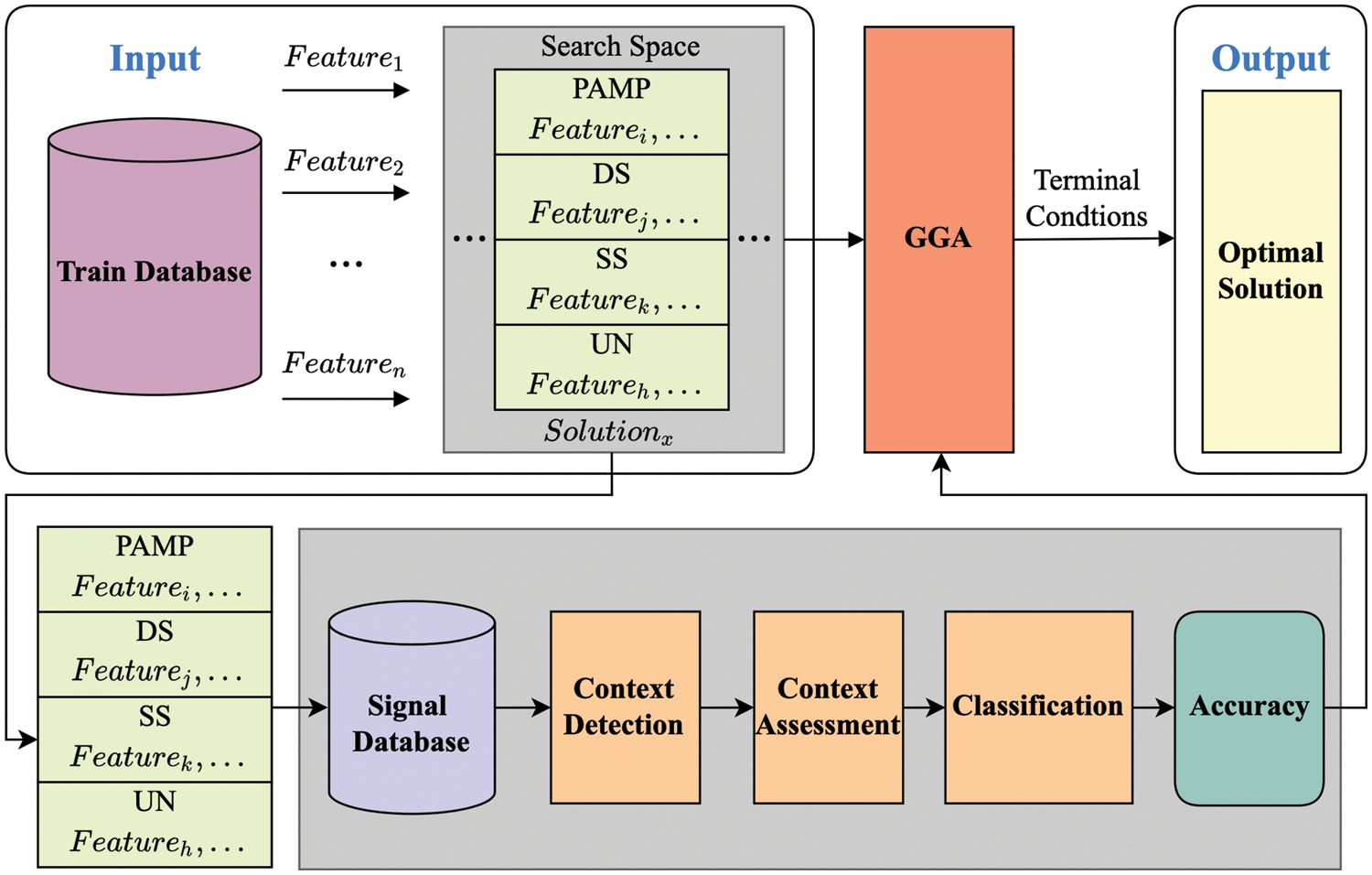
Figure 1: The model of GGA-DCA
As shown in Fig. 2, the work of signal categorization is to establish a mapping relationship between selected features and signal categories, offered as Eq. (3). Establishing a mapping relation can be considered as dividing the attributes into different groups.
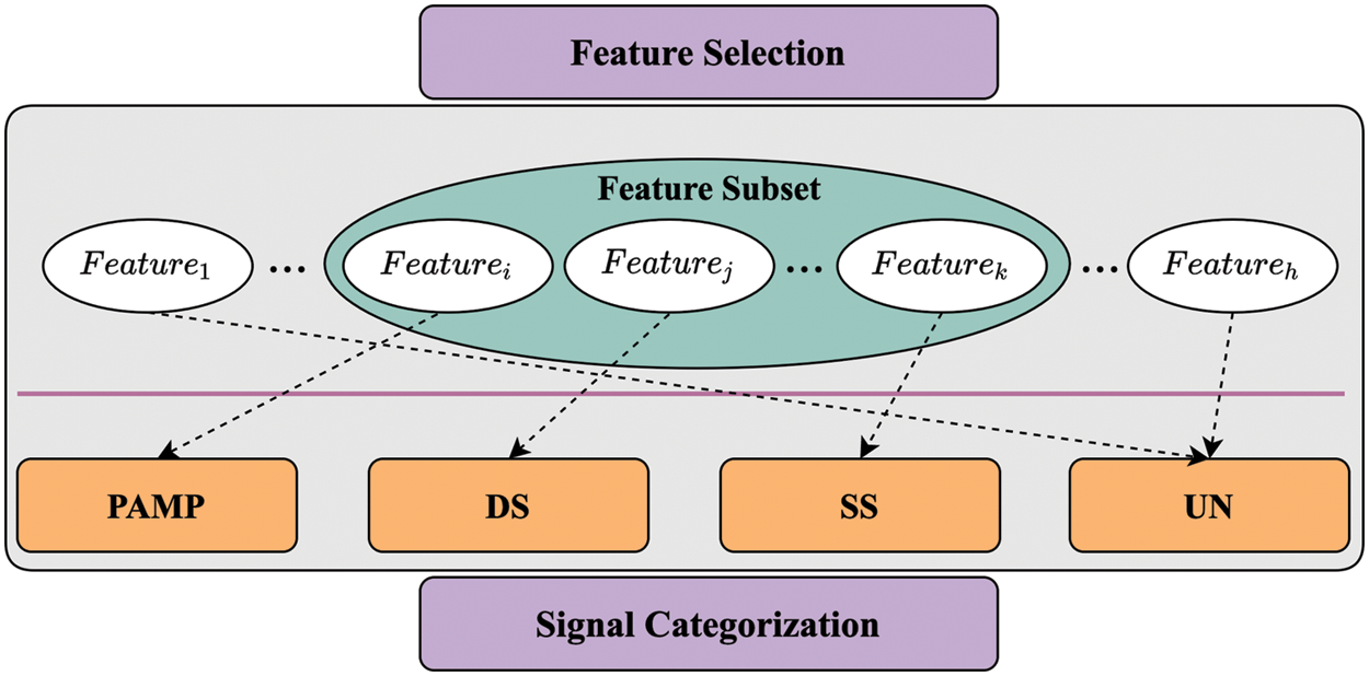
Figure 2: Steps of feature selection and signal categorization
The grouping scheme of the features is a solution to feature selection and signal classification, as shown in Fig. 3. In this study, the solution can be denoted as

Figure 3: The grouping scheme: A 4-dimensional vector V
In this work, the classification accuracy of DCA is adopted to evaluate the performance of states. A signal database contributed by a state is performed multiple times, and the average accuracy of multiple experiments is the performance of a state.
This study employs GGA as the search engine to find the optimal feature grouping scheme. The key steps are as described below.
Step 1: Data encoding. In GGA, each chromosome represents a state in the search space. The nature of the problem determines the chromosome coding [29]. This study uses integers {i, j, k, h, …} to represent independent features separately {
Step 2: Fitness function. The fitness function of a given chromosome determines its probability of being chosen to create the next generation [29]. This study adopts the classification accuracy of DCA, that described in Section 3.2, to evaluate the performance of a chromosome.
where V is a chromosome, fitness (V) is the fitness value of chromosome V. Accuracy(DCA(V)) is the mean of classification accuracy achieved by DCA running multi-times on a signal database generated through the chromosome V.
Step 3: Selection function. After computing the fitness for each chromosome in the current population, the better ones need to be selected as the next generation’s parents by utilizing the roulette wheel. The cumulative fitness values of all the chromosomes in each iteration are calculated. A chromosome is selected with a probability equaling the proportion of its fitness value in the cumulative, shown in Eq. (5).
where
Step 4: Crossover operator. In this work, the chromosomes with different orders of groups are unique. To explore the more possible chromosomes around the current one, 1PX (One-point Crossover) [27] is utilized to swap the groups of two chromosomes randomly. The crossover is performed on a randomly selected chromosome with a probability
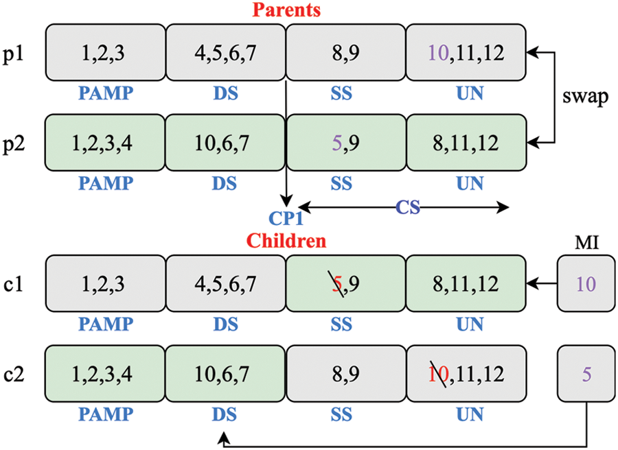
Figure 4: The crossover operators of GGA-DCA
Step 5: Mutation operator. The operator transforms one chromosome into another by swapping genes of two existing groups in the chromosome. This study performs mutation with a probability
Step 6: Termination conditions. The search process is running iteratively until satisfying one of the two conditions. The first condition is when the fitness value of a chromosome is more significant than a threshold. The second condition is when the generations of populations execute up to a certain number G.
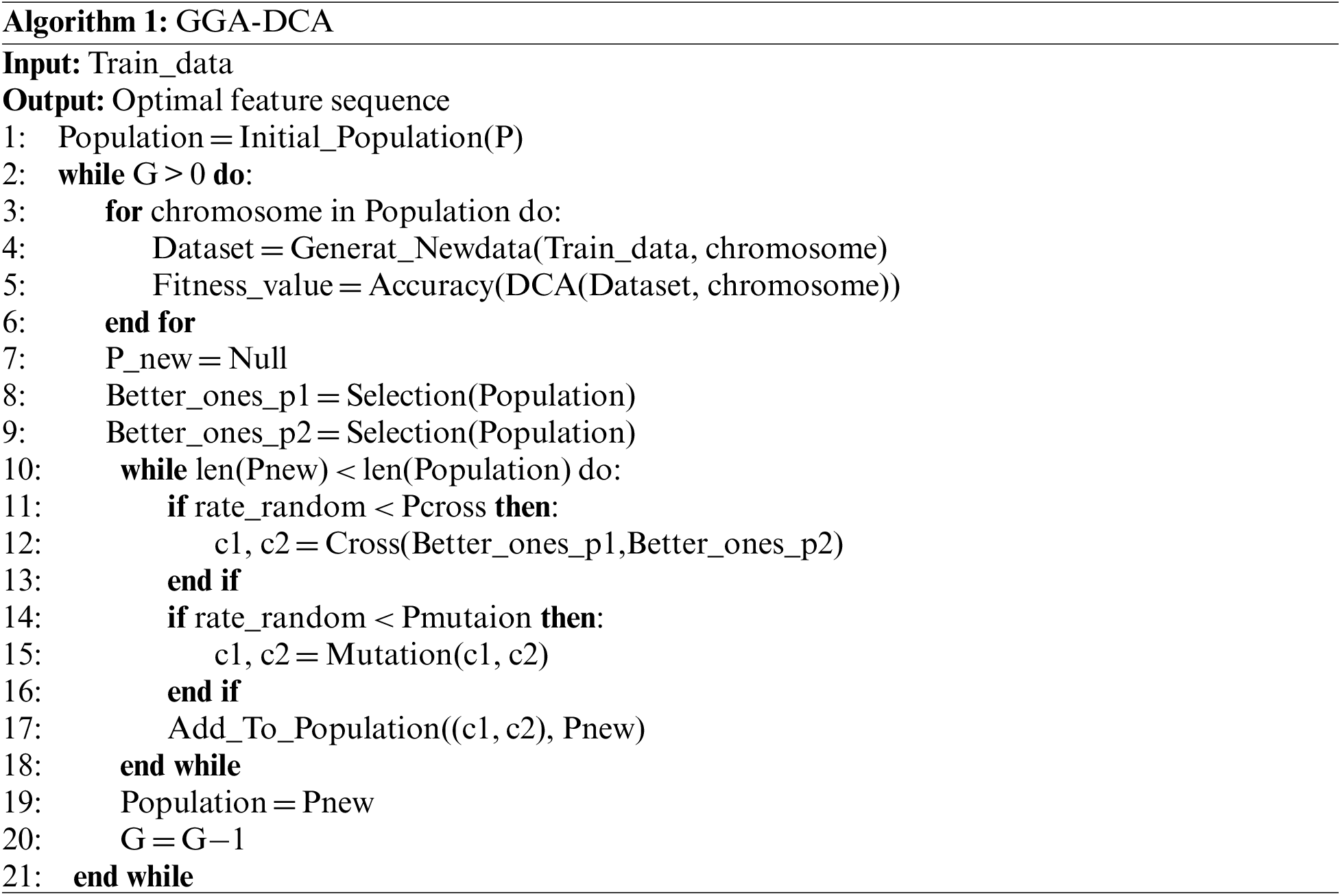
Step 7: Algorithm of GGA-DCA. The search process of GGA for an optimal solution is illustrated in Algorithm 1. In algorithm, the first step is to initialize a population. For initializing, the data set features are randomly mapped to the group schemes of P chromosomes in a population to generate P input signal data sets. After initializing, the fitness values of all chromosomes in the population are computed and stored in memory. To expand the searching scope, the genetic operators are applied to the current population to generate the next generation population
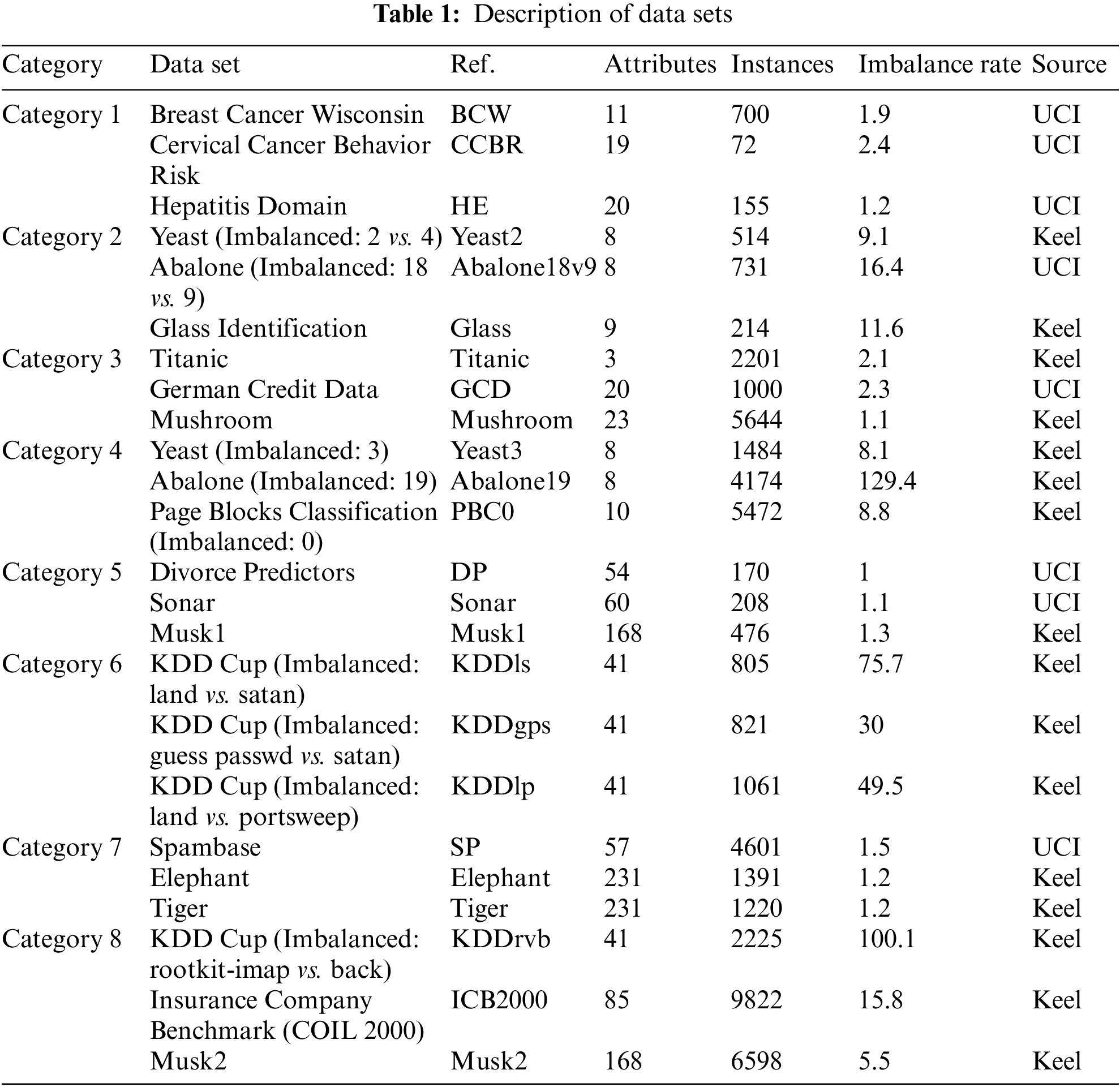
To verify the performance of the proposed GGA-DCA, twenty-four different classification problems from UCI Machine Learning Repository [32], Keel [33], are used for experiments. Those data sets, shown in Table 1, are selected according to the level of feature dimensions, the size of the dataset, and the level of the imbalance rate. Those data sets are divided into eight categories; Category 1: balanced small-sized low-dimensional data sets; Category 2: imbalanced small-sized low-dimensional data sets; Category 3: balanced large-sized low-dimensional data sets; Category 4: imbalanced large-sized low-dimensional data sets; Category 5: balanced small-sized high-dimensional data sets; Category 6: imbalanced small-sized high-dimensional data sets; Category 7: balanced large-sized high-dimensional data sets; Category 8: imbalanced large-sized high-dimensional data sets. Each category contains three data sets so that the performance of GGA-DCA can be fully tested by performing classification tasks on these 24 data sets. In this work, non-numerical features are transformed into numerical features. Before experiments, this study filters the features with a high percentage of missing values and the features with a single unique value. The data imputation techniques may not work well for data sets with a high rate of missing values. Thus, this study filters those features which are missing more than 40% of data. Those features with a single unique value cannot be useful for machine learning because of their zero variance. Thus, this study counts unique values for each attribute in a data set. The features with one unique value are filtered. Due to the significant effect of influential points on the algorithm, this study replaces these influential points with the mean. Thus, this study utilizes the Z-score method to look for influential points, shown in Eq. (6). This study filters those features whose
where
In this work, two experiments are performed to study the feasibility and superiority of the proposed approach. In the first experiment, GGA-DCA and state-of-the-art DCA expansion algorithms (NIDDCA [1], FLA-DCA [17], GA-PSM [29], and the SVM-DCA [20]) perform classification tasks on the 24 data sets. For the purpose of baseline comparison, the well-known classifiers, the KNN, the DT, the XGboost, the RF, and the ERT, also perform classification tasks on the 24 data sets. Each data set is divided into two disjoint sets: training (80%) and testing (20%). In all experiments, ten independent runs of each algorithm are conducted based on the 10-fold cross-validation method. To evaluate the performance of the above approaches, the accuracy, precision, specificity, F-measure, and the area under the curve (AUC), are calculated for all the data sets. Accuracy is a proportion of the correct predictions on all items. Precision is a proportion of positive items on all cases labeled normal. The specificity is the percentage of positive cases on all correct cases. F-measure is a harmonic mean of precision and recall. All experiments are performed on a laptop with Intel Core i7-5600U 2.6 GHz-8 GB RAM-HP running Windows 10. Those approaches are implemented in Python using PyCharm.
In this work, the size of the DC poll is 100, and each antigen samples up to 10 data items. The migration threshold is the combination of the weight values and the max signal values using Eq. (1). For classification, this study adopts the proportion of the abnormal items in a data set as the threshold of MCAV. The weights of DCA are adjusted through the feedback adjustment method of NIDDCA [1]. The iterations (G) and the population size of GGA-DCA using GGA are both 10 in each experiment. The probability
The GGA-DCA wraps a search task around the DCA. The runtime of DA-DCA depends on the iteration number of GGA, the chromosome number of each generation, and the runtime of DCA. The calculation of the runtime is performed phase by phase. According to work in Gu et al. [34], the runtime complexity of DCA is bounded by
where P is the population’s size, G is the number of iterations, n is the data size,
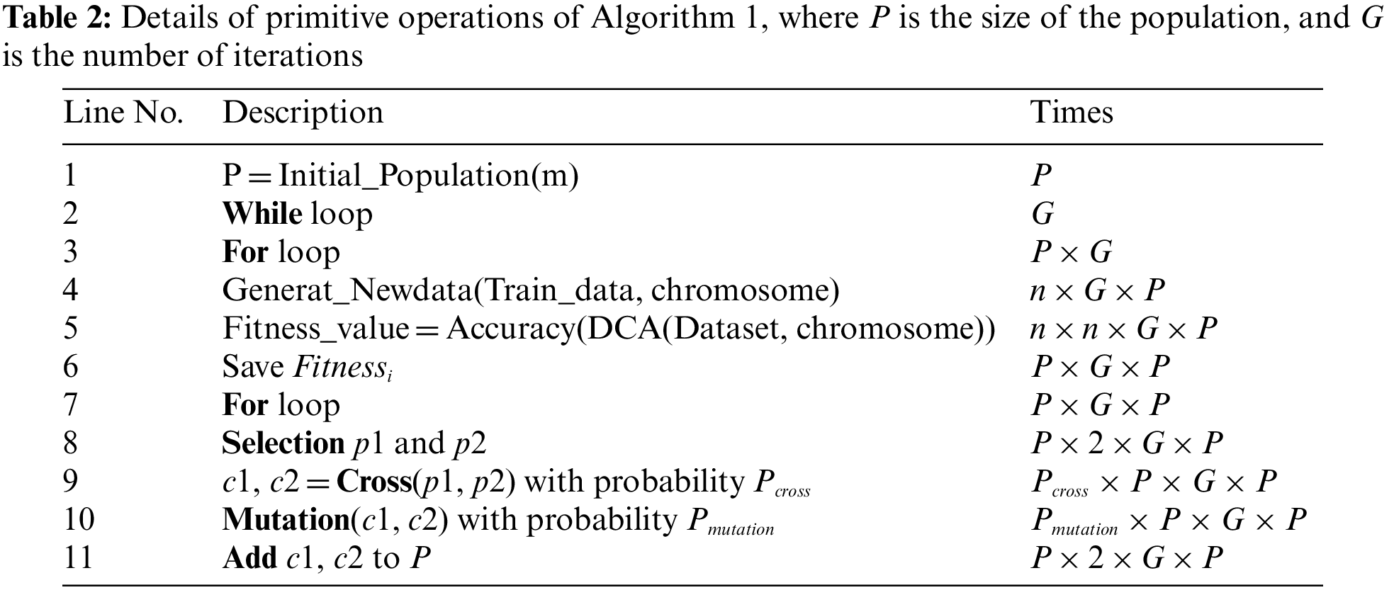
As shown in Eq. (12), GGA-DCA has a worse case runtime complexity of
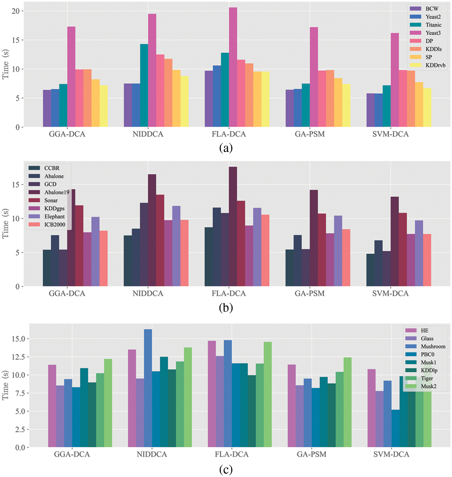
Figure 5: Mean execution time (in seconds) acquired by DCA versions (e.g., GGA-DCA, NIDDCA, FLADCA, GA-PSM, SVM-DCA)
5.5 Results Analysis and Comparison
For all the data sets, this study computes the mean and standard deviations of the accuracy obtained by the ten algorithms (GGA-DCA, NIDDCA, FLA-DCA, SVM-DCA, GA-PSM, KNN, DT, XGboost, RF, and ERT), and the results are shown in Table 3. The Table 4 shows the mean and standard deviations of precision obtained by those ten algorithms. Moreover, the specificity, F-Measure, and AUC of the ten algorithms are also calculated based on the 24 data sets, and the results are respectively presented in Tables 5, 6 and 7. The number in bold represents the best result among the then algorithms in all the tables.
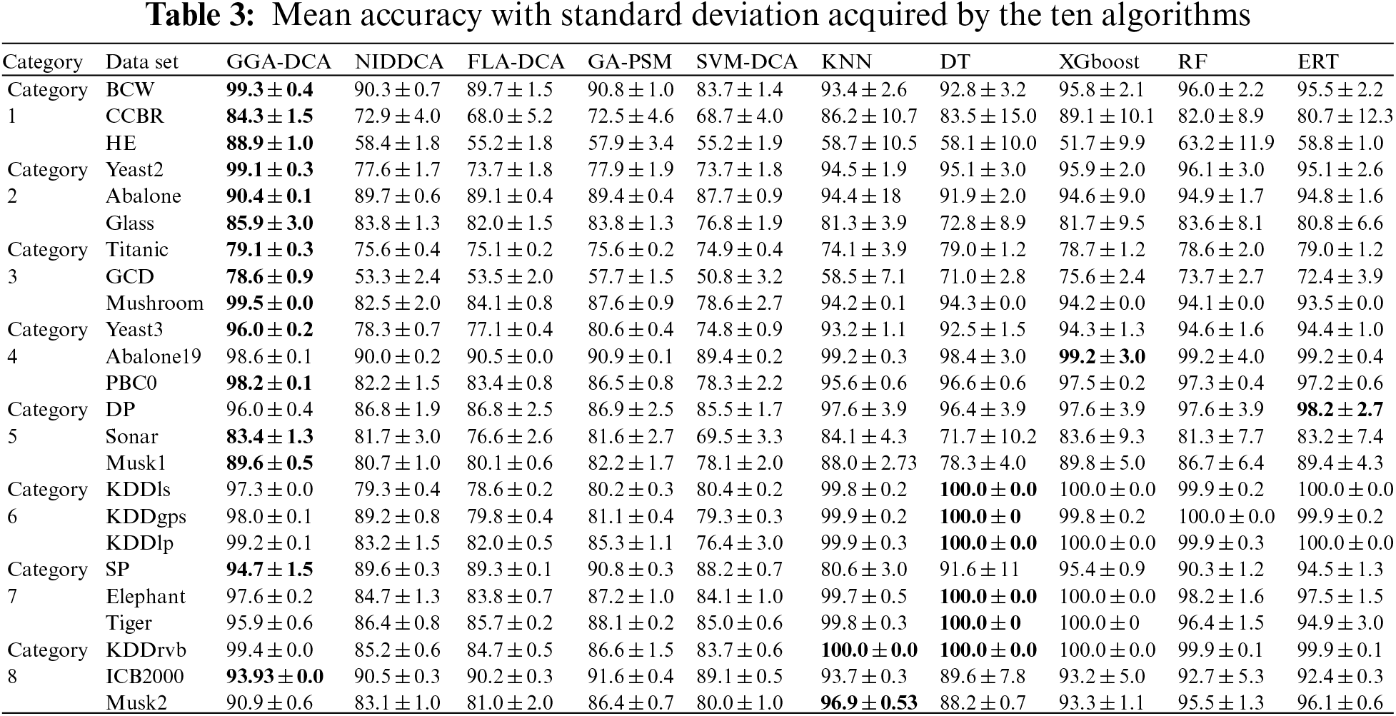
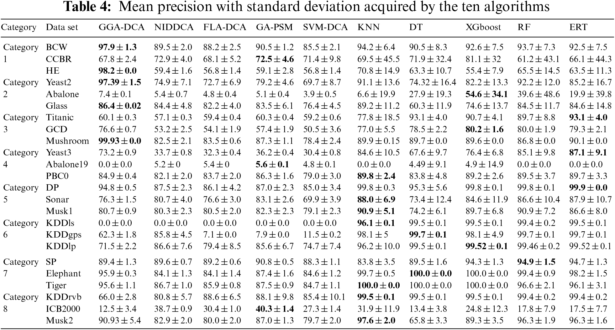
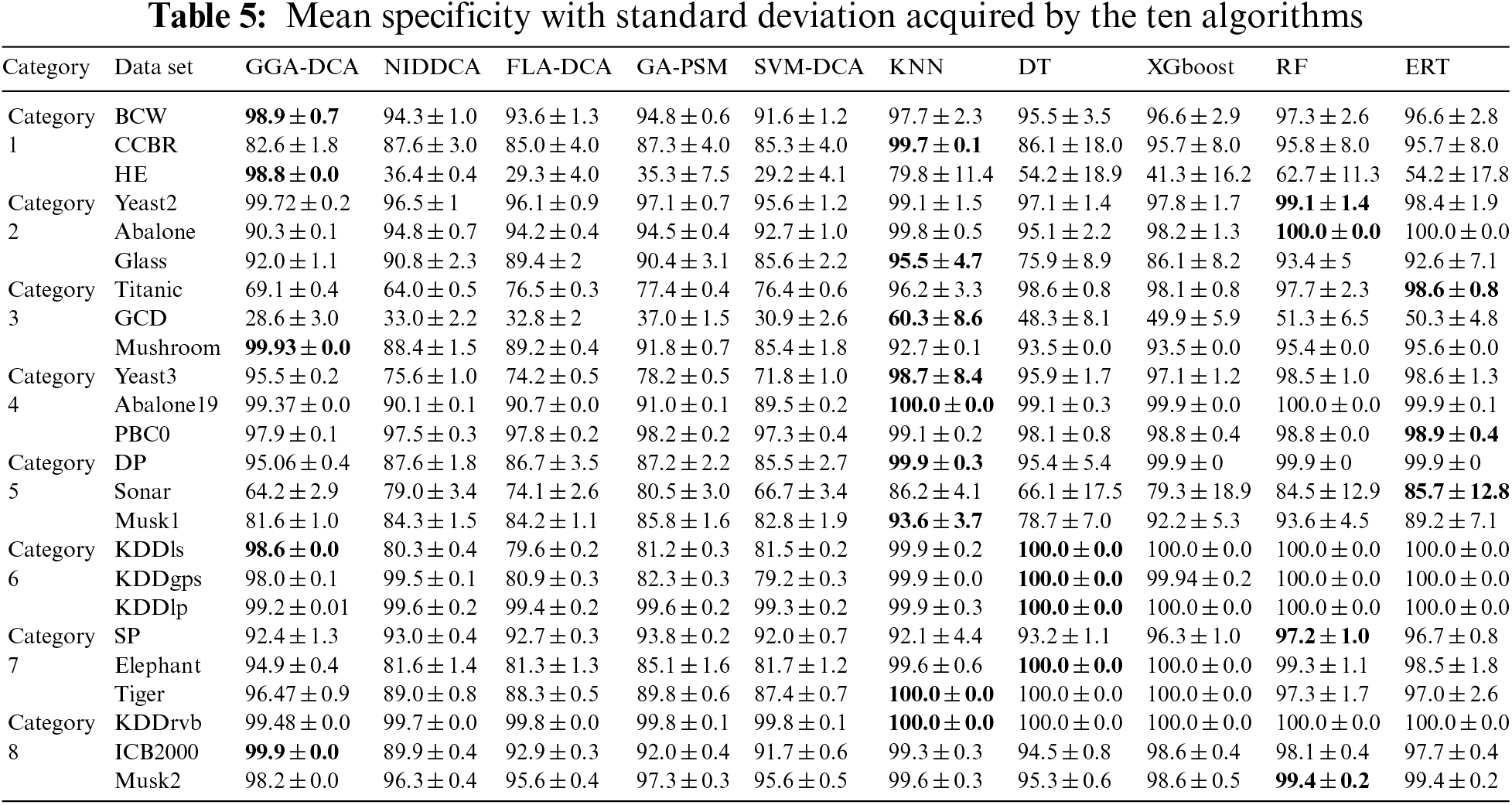
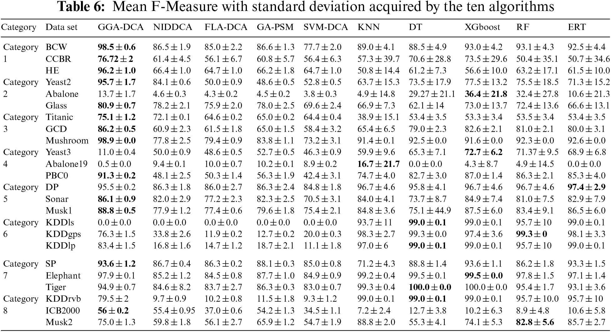
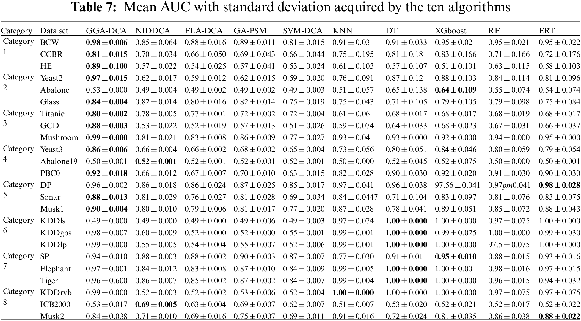
The Tables 3–7 show that the proposed GGA-DCA consistently achieves better performance on the 24 data sets compared with DCA versions (e.g., NIDDCA, FLA-DCA, SVM-DCA, and GA-PSM). We can conclude that the proposed GGA-DCA is superior to the state-of-the-art DCA versions (e.g., NIDDCA, FLA-DCA, SVM-DCA, and GA-PSM) over all the UCI and Keel data sets in a statistically significant manner. Moreover, the Table 3 also shows that the GGA-DCA obtains better classification accuracy compared with those machine learning algorithms, e.g., KNN, DT, XGboost, RF, and ERT, on those data sets with low-dimensional feature space (e.g., BCW, CCBR, HE, Yeast2, Abalone, Glass, Titanic, GDD, Yeast3, and PBC0). When performing classification on those data sets with high-dimensional feature space (e.g., Musk2, Tiger, and Elephant), the proposed GGA-DCA has not obtained the same satisfactory results as machine learning algorithms. However, our method maintains the same advantage as those machine learning algorithms in terms of AUC.
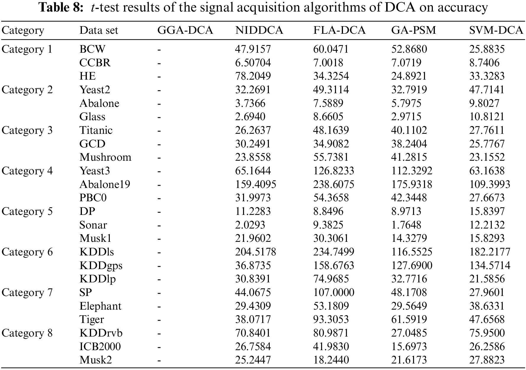
To better analyze the results, this study tests the following hypotheses using the t-test to analyze whether significant differences exist in the experiments between the GGA-DCA and other signal acquisition algorithms of DCA (called “Comparisons”) under the condition z = 0.05.
The Table 8 shows the t-test results on accuracy. When the degree of freedom is nine, and the significance level of the t-test is 0.05, the critical t-value is 2.262. Therefore, if the result is below 2.262, we can conclude that
This study firstly provides formal definitions of the DCA, such as DCs, inputs, and outputs, to make researchers understand the algorithm better. The works of feature selection and signal categorization are analyzed. Inspired by the grouping problems, this study models those works into a feature grouping problem. By searching for the optimal grouping scheme, this study automatically accomplishes feature selection and signal categorization without any expertise. The GGA is introduced to perform the searching task without expertise, making the algorithm more adaptive to apply to more fields. This study mixes the GGA and DCA to form a novel DCA version, GGA-DCA, to automatically accomplish feature selection and signal categorization. This study redefined crossover and mutation in GGA and let it find the optimal grouping with the most less time for DCA. The classification results from experiments indicate that GGA-DCA generally finds the optimal grouping schemes and keeps the algorithm lightweight in terms of running time without expertise.
The future works include two parts. Firstly, more search methods will be explored to perform feature selection and signal categorization, such as Monarch Butterfly Optimization (MBO) [35], Elephant Herding Optimization (EHO) [36], Krill Herd (KH) [37], and three-phase search approach with dynamic population size (TPSDP) [38]. Secondly, other metrics will be attempted to measure the performance of a feature grouping. The F-measure is the weighted harmonic average of precision and recall, which can measure the performance better. Hence, the F-measure is the next evaluation indicator for GGA-DCA.
Funding Statement: The authors want to thank NSFC http://www.nsfc.gov.cn/ for the support through Grants No. 61877045, and Fundamental Research Project of Shenzhen Science and Technology Program for the support through Grants No. JCYJ2016042815-3956266.
Conflicts of Interest: The authors declare that they have no conflicts of interest to report regarding the present study.
References
1. Zhou, W., Liang, Y. (2021). A new version of the deterministic dendritic cell algorithm based on numerical differential and immune response. Applied Soft Computing, 102, 107055. DOI 10.1016/j.asoc.2020.107055. [Google Scholar] [CrossRef]
2. Greensmith, J., Aickelin, U. (2008). The deterministic dendritic cell algorithm. In: Artificial immune systems, vol. 5132. Phuket, Thailand: lNCS. [Google Scholar]
3. Dagdia, Z. C. (2019). A scalable and distributed dendritic cell algorithm for big data classification. Swarm and Evolutionary Computation, 50, 100432. DOI 10.1016/j.swevo.2018.08.009. [Google Scholar] [CrossRef]
4. Zhang, C., Yi, Z. (2010). A danger theory inspired artificial immune algorithm for on-line supervised two-class classification problem. Neurocomputing, 73(7), 1244–1255. DOI 10.1016/j.neucom.2010.01.005. [Google Scholar] [CrossRef]
5. Abdelhaq, M., Hassan, R., Alsaqour, R. (2011). Using dendritic cell algorithm to detect the resource consumption attack over manet. International Conference on Software Engineering and Computer Systems, pp. 429–442. Berlin, Heidelberg, Springer. [Google Scholar]
6. Farzadnia, E., Shirazi, H., Nowroozi, A. (2021). A novel sophisticated hybrid method for intrusion detection using the artificial immune system. Journal of Information Security and Applications, 58, 102721. DOI 10.1016/j.jisa.2020.102721. [Google Scholar] [CrossRef]
7. El-Alfy, E. S. M., Al-Hasan, A. A. (2014). A novel bio-inspired predictive model for spam filtering based on dendritic cell algorithm. 2014 IEEE Symposium on Computational Intelligence in Cyber Security (CICS), Florida, USA, IEEE. [Google Scholar]
8. Chen, W., Zhao, H., Li, T., Liu, Y. (2018). Optimal probabilistic encryption for distributed detection in wireless sensor networks based on immune differential evolution algorithm. Wireless Networks, 24(7), 2497–2507. DOI 10.1007/s11276-017-1484-3. [Google Scholar] [CrossRef]
9. Zhou, W., Liang, Y., Ming, Z., Dong, H. (2020). Earthquake prediction model based on danger theory in artificial immunity. Neural Network World, 30(4), 231–247. DOI 10.14311/NNW.2020.30.016. [Google Scholar] [CrossRef]
10. Chelly, Z., Elouedi, Z. (2016). A survey of the dendritic cell algorithm. Knowledge and Information Systems, 48(3), 505–535. DOI 10.1007/s10115-015-0891-y. [Google Scholar] [CrossRef]
11. Gu, F., Greensmith, J., Oates, R., Aickelin, U. (2009). PCA 4 DCA: The application of principal component analysis to the dendritic cell algorithm. 9th Annual Workshop on Computational Intelligence (UKCI 2009), Nottingham, UK. [Google Scholar]
12. Gu, F. (2011). Theoretical and empirical extensions of the dendritic cell algorithm (Ph.D. Thesis). University of Nottingham. [Google Scholar]
13. Chelly, Z., Elouedi, Z. (2012). RST-DCA: A dendritic cell algorithm based on rough set. International Conference on Neural Information Processing, pp. 480–487. Berlin, Heidelberg: Springer. [Google Scholar]
14. Chelly, Z., Elouedi, Z. (2012). RC-DCA: A new feature selection and signal categorization technique for the dendritic cell algorithm based on rough set theory. Artificial Immune Systems. 11th International Conference, vol. 7597. Taormina, Italy, LNCS. [Google Scholar]
15. Chelly, Z., Elouedi, Z. (2013). QR-DCA: A new rough data pre-processing approach for the dendritic cell algorithm. In: Adaptive and natural computing algorithms, vol. 7824. Lausanne, Switzerland, LNCS. [Google Scholar]
16. Chelly, Z., Elouedi, Z. (2013). A fuzzy-rough data pre-processing approach for the dendritic cell classifier. In: Symbolic and quantitative approaches to reasoning with uncertainty, pp. 109–120. Berlin, Heidelberg: LNAI, Springer. [Google Scholar]
17. Chelly, Z., Elouedi, Z. (2013). Supporting fuzzy-rough sets in the dendritic cell algorithm data pre-processing phase. In: Neural information processing, vol. 8227. Berlin, Heidelberg: LNCS, Springer. [Google Scholar]
18. Kohavi, R., John, G. H. (1997). Wrappers for feature subset selection. Artificial Intelligence, 97(1–2), 273–324. DOI 10.1016/S0004-3702(97)00043-X. [Google Scholar] [CrossRef]
19. Ali, K. B., Chelly, Z., Elouedi, Z. (2015). A new version of the dendritic cell immune algorithm based on the k-nearest neighbors. Neural Information Processing. 22nd International Conference (ICONIP 2015), vol. 9489. Cham, LNCS, Springer International Publishing. [Google Scholar]
20. Mohsin, M. F., Hamdan, A. R., Bakar, A. A. (2014). An evaluation of feature selection technique for dendrite cell algorithm. 2014 International Conference on IT Convergence and Security (ICITCS), Beijing, China. [Google Scholar]
21. Feng, Y., Wang, G. G. (2022). A binary moth search algorithm based on self-learning for multidimensional knapsack problems. Future Generation Computer Systems, 126, 48–64. DOI 10.1016/j.future.2021.07.033. [Google Scholar] [CrossRef]
22. Zhuang, Z., Huang, Z., Lu, Z., Guo, L., Cao, Q. et al. (2019). An improved artificial bee colony algorithm for solving open shop scheduling problem with two sequence-dependent setup times. Procedia CIRP, 83, 563–568. DOI 10.1016/j.procir.2019.04.119. [Google Scholar] [CrossRef]
23. Wang, G. G., Gao, D., Pedrycz, W. (2022). Solving multi-objective fuzzy job-shop scheduling problem by a hybrid adaptive differential evolution algorithm. IEEE Transactions on Industrial Informatics, DOI 10.1109/TII.2022.3165636. [Google Scholar] [CrossRef]
24. Gao, S., Wang, K., Tao, S., Jin, T., Dai, H. et al. (2021). A state-of-the-art differential evolution algorithm for parameter estimation of solar photovoltaic models. Energy Conversion and Management, 230, 113784. DOI 10.1016/j.enconman.2020.113784. [Google Scholar] [CrossRef]
25. Baniamerian, A., Bashiri, M., Tavakkoli-Moghaddam, R. (2019). Modified variable neighborhood search and genetic algorithm for profitable heterogeneous vehicle routing problem with cross-docking. Applied Soft Computing, 75, 441–460. DOI 10.1016/j.asoc.2018.11.029. [Google Scholar] [CrossRef]
26. Pakzad-Moghaddam, S. (2016). A levy flight embedded particle swarm optimization for multi-objective parallel-machine scheduling with learning and adapting considerations. Computers & Industrial Engineering, 91, 109–128. DOI 10.1016/j.cie.2015.10.019. [Google Scholar] [CrossRef]
27. Ramos-Figueroa, O., Quiroz-Castellanos, M., Mezura-Montes, E., Kharel, R. (2021). Variation operators for grouping genetic algorithms: A review. Swarm and Evolutionary Computation, 60, 100796. DOI 10.1016/j.swevo.2020.100796. [Google Scholar] [CrossRef]
28. Ramos-Figueroa, O., Quiroz-Castellanos, M., Mezura-Montes, E., Schutze, O. (2020). Metaheuristics to solve grouping problems: A review and a case study. Swarm and Evolutionary Computation, 53, 100643. DOI 10.1016/j.swevo.2019.100643. [Google Scholar] [CrossRef]
29. Elisa, N., Yang, L., Chao, F. (2020). Signal categorisation for dendritic cell algorithm using ga with partial shuffle mutation. In: Advances in computational intelligence systems, vol. 1043. Germany: AISC, Springer. [Google Scholar]
30. Gao, D., Wang, G. G., Pedrycz, W. (2020). Solving fuzzy job-shop scheduling problem using de algorithm improved by a selection mechanism. IEEE Transactions on Fuzzy Systems, 28(12), 3265–3275. DOI 10.1109/TFUZZ.91. [Google Scholar] [CrossRef]
31. Falkenauer, E. (1993). The grouping genetic algorithms: Widening the scope of the GAs. Belgian Journal of Operations Research, Statistics, and Computer Science, 33(1–2), 79–102. [Google Scholar]
32. Asuncion, A., Newman, D. (2007). UCI machine learning repository. University of California, Irvine, USA: Dua, Dherru and Graff, Casey. [Google Scholar]
33. Alcala-Fdez, J., Fernández, A., Luengo, J., Derrac, J., Garc’ia, S. et al. (2010). Keel data-mining software tool: Data set repository, integration of algorithms and experimental analysis framework. Journal of Multiple-Valued Logic and Soft Computing, 17, 255–287. [Google Scholar]
34. Gu, F., Greensmith, J., Aickelin, U. (2013). Theoretical formulation and analysis of the deterministic dendritic cell algorithm. Biosystems, 111(2), 127–135. [Google Scholar]
35. Wang, G. G., Deb, S., Cui, Z. (2019). Monarch butterfly optimization. Neural Computing & Applications, 31(7), 1995–2014. [Google Scholar]
36. Li, W., Wang, G. G., Alavi, A. H. (2020). Learning-based elephant herding optimization algorithm for solving numerical optimization problems. Knowledge-Based Systems, 195, 105675. [Google Scholar]
37. Wang, G. G., Guo, L., Gandomi, A. H., Hao, G. S., Wang, H. (2014). Chaotic krill herd algorithm. Information Sciences, 274, 17–34. [Google Scholar]
38. Yang, X., Cai, Z., Jin, T., Tang, Z., Gao, S. (2022). A Three-phase search approach with dynamic population size for solving the maximally diverse grouping problem. European Journal of Operational Research, 302(3), 925–953. [Google Scholar]
Cite This Article
 Copyright © 2023 The Author(s). Published by Tech Science Press.
This work is licensed under a Creative Commons Attribution 4.0 International License , which permits unrestricted use, distribution, and reproduction in any medium, provided the original work is properly cited.


 Submit a Paper
 Propose a Special lssue
 View Full Text
 Download PDF
 Downloads
 Citation Tools