Ranked-Set Sampling Based Distribution Free Control Chart with Application in CSTR Process

1  Introduction

The statistical process control (SPC) toolkit collects various statistical tools used to monitor the production and service processes. Control charts are one of the most important tools in the SPC toolkit for detecting changes in process parameters (location and/or dispersion). There are numerous control charts for efficient process monitoring in the SPC literature. Shewhart [1] introduced the basic control charts, called the Shewhart control charts. These control charts are also known as memoryless control charts because they only use current process information. Although the Shewhart control charts are simple to design and implement, they are less sensitive for small to moderate shifts detection. The other control charts that are more sensitive than the Shewhart control charts are the Cumulative sum (CUSUM) control chart, introduced by Page [2], and the exponentially weighted moving average (EWMA) control chart suggested by Roberts [3]. The CUSUM and EWMA control charts are also called the memory control chart, as these control charts use both current and previous information about the process.

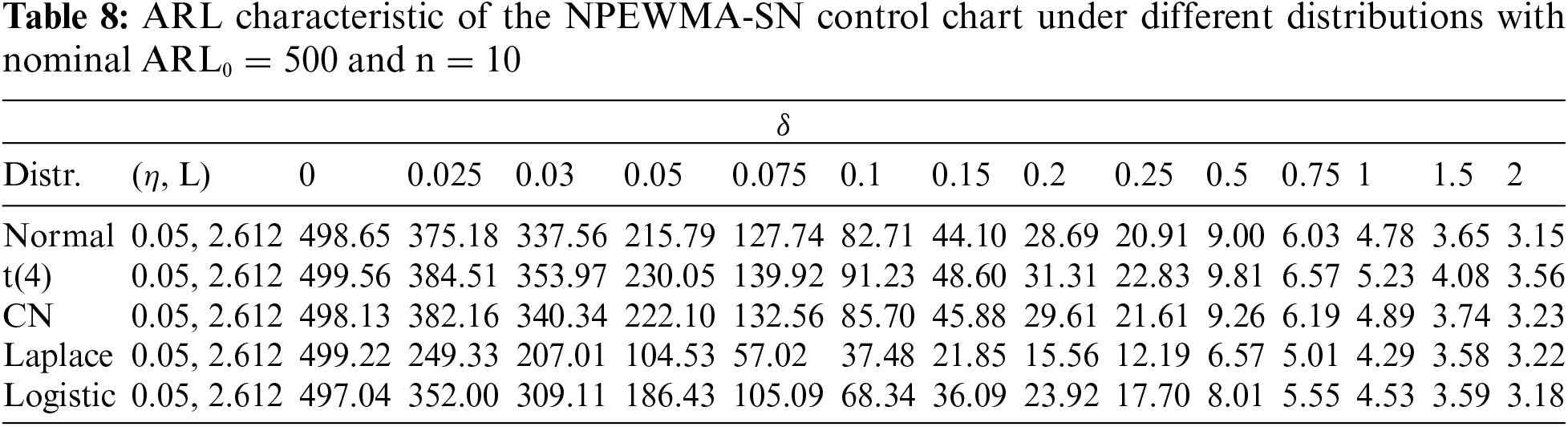
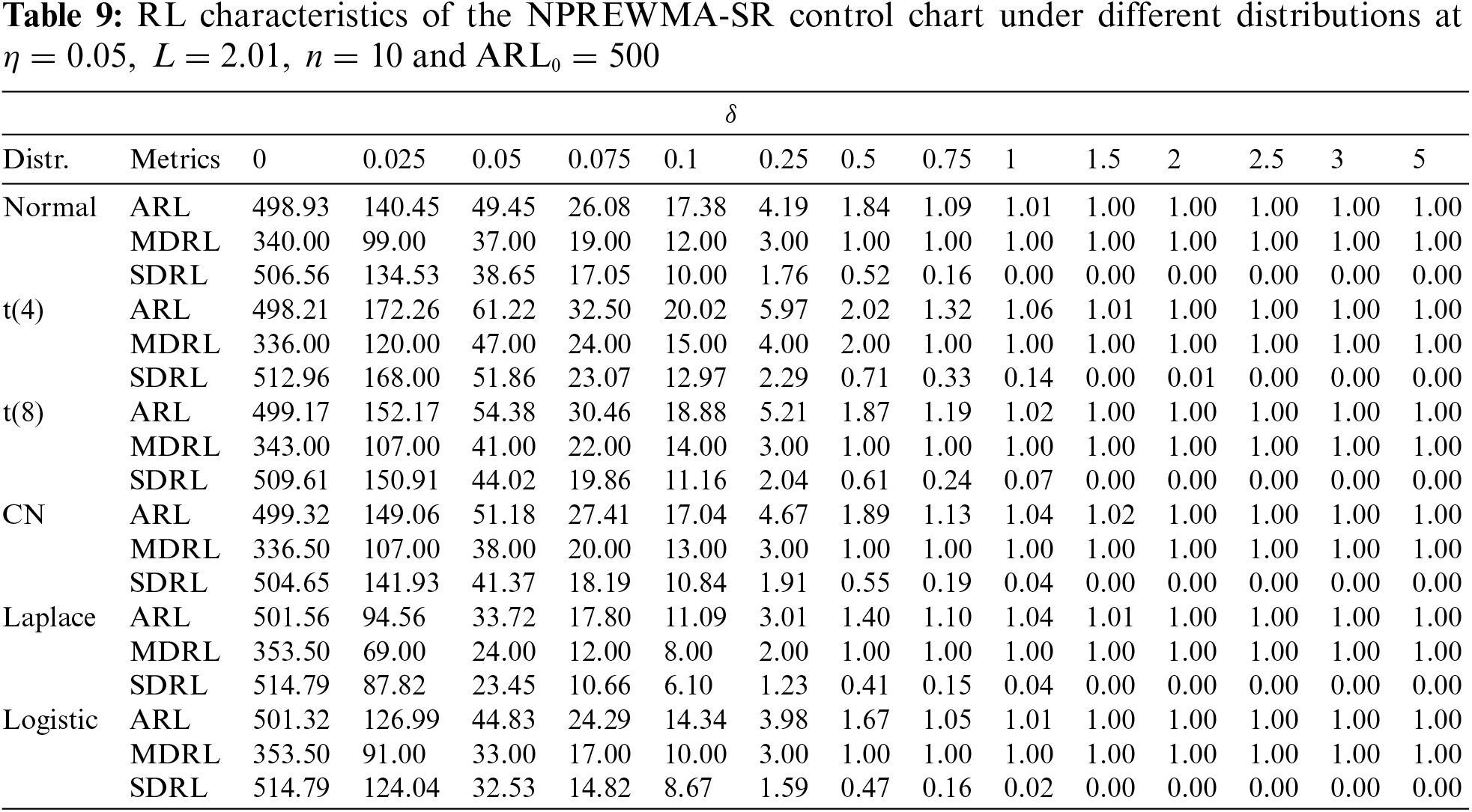
Generally, it is assumed that the process often follows a specific distribution. When this assumption is violated, the quality of these objects may be affected. Nonparametric (NP) control charts are used in this scenario because they do not require the assumption of specified distribution. In addition, the population variance is unnecessary when employing NP control charts to observe the shifts in the process location. The sign (SN) and Wilcoxon signed-rank (SR) are commonly used NP techniques in the control charts context. For instance, Yang et al. [4] studied the NP EWMA sign (NPEWMA-SN) control chart for monitoring shifts in process location. Similarly, Graham et al. [5] and Graham et al. [6] investigated single observation-based NP EWMA sign and NP EWMA signed-rank control charts to monitor process location, respectively. Likewise, Chakraborty et al. [7] introduced the generally weighted moving average SN (GWMA-SN) control chart to detect the process location shifts. Later, Abid et al. [8] offered the ranked set sampling (RSS) based NP EWMA Wilcoxon signed-rank (NPREWMA-SR) control chart for monitoring shifts in process location efficiently. Moreover, Ali et al. [9] recommended NP control charts to detect location parameter changes. Also, Ali et al. [9] designed the RSS-based NP EWMA SN (NPREWMA-SN) control chart for monitoring shifts in process location.

The CUSUM and EWMA types schemes and modified versions are used for efficient process monitoring. For instance, Lucas et al. [10] offered the combined Shewhart-EWMA (CS-EWMA) control chart to enhance the shift detection ability in the process location. Similarly, Shamma et al. [11] proposed a double EWMA (DEWMA) chart, outperforming the EWMA control chart in early process location shifts detection. Likewise, Zhang et al. [12] introduced the DEWMA chart’s run length (RL) features. They suggested that DEWMA and EWMA charts are equally beneficial for detecting large shifts in process parameters. Later, Abbas et al. [13] and Zaman et al. [14] designed the mixed EWMA-CUSUM (MEC) and mixed CUSUM-EWMA (MCE) charts, respectively, to efficiently monitor process location shifts. Also, Anwar et al. [15] suggested auxiliary information-based (AIB) MEC and MCE control charts for monitoring the process location parameter. For other CUSUM and EWMA based studies, the readers are referred to the work of Adegoke et al. [16], Sanusi et al. [17], Haq [18], Zaman et al. [19], Aslam et al. [20], Adeoti et al. [21], Anwar et al. [15], Abbasi et al. [22], Rasheed et al. [23], Rasheed et al. [24], Anwar et al. [25], Liu et al. [26], and Rasheed et al. [27].

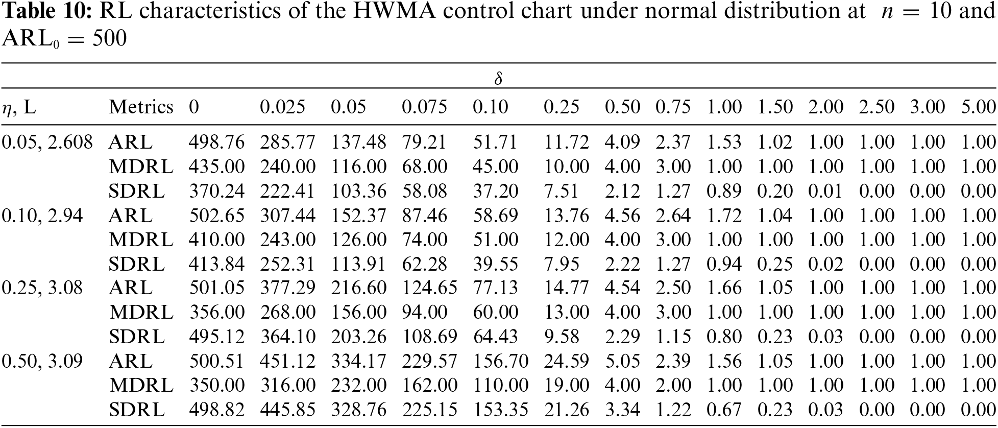
Hunter [28] noticed that the EWMA control chart assigns a higher weight to current observations and less weight to prior observations of the process. Later, Abbas [29] proposed the homogeneously weighted moving average (HWMA) control chart for observing shifts in process location. After that, Abid et al. [30] introduced the mixed HWMA-CUSUM (MHC) control chart for monitoring shifts in the process location. Similarly, Adeoti et al. [31] advocated a hybrid HWMA (HHWMA) control chart to detect the process location shifts. In addition, Abid et al. [32] offered the double HWMA (DHWMA) control chart to observe process location shifts. They showed that the DHWMA control chart has better detection ability than the HWMA control chart. Recently, Anwar et al. [33] suggested an AIB DHWMA control chart for improved process location monitoring.

Simple random sampling (SRS) and perfect RSS are frequently used in SPC to monitor underlying process data. These sampling techniques are commonly used with parametric and nonparametric control charts. However, when actual measurements are difficult to obtain, or the cost of sampling is prohibitively expensive, the RSS should be used instead of SRS. Ranking errors can impact estimator performance and result in ambiguous estimates. Dell et al. [34] studied the impacts of inaccuracy and imperfect RSS on the performance of mean estimators. They claim that the RSS mean estimator remains unbiased when imperfect ranking is used and outperforms the SRS estimator. Besides that, the RSS’s efficiency remains higher than that of the imperfect RSS and SRS. Numerous NP HWMA type control charts based on simple random sampling (SRS) are available. Still, according to the author’s knowledge, no NP HWMA control chart based on perfect and imperfect RSS is present in the literature. Capitalizing this research gap, this article introduces an NP HWMA SR control chart with perfect and imperfect RSS (NPHWMARSS) for monitoring process location shifts for continuous and symmetric distributions. The performance measures, such as average run length (ARL), median run length (MDRL), and standard deviation of run-length (SDRL), are computed under different distributions, including the normal, student’s t, contaminated normal (CN), Laplace, and logistic distributions. Based on these performance measures, the proposed NPHWMARSS control chart is compared to the competing control charts, such as EWMA, NPEWMA-SR, NPEWMA-SN, NPREWMA-SR, and HWMA control charts. The comparison indicates the superiority of proposed NPHWMARSS control chart over the competing control charts in small to moderate shift detection.

The remainder of the paper is structured as follows: Section 2 offers the proposed control chart’s methodology and design and the competing control chart. Section 3 evaluates the IC and OOC performance of the proposed NPHWMARSS control chart. Section 4 covers a comparative study of the proposed NPHWMARSS chart, whereas Section 5 addresses a real-life application. Lastly, Section 6 provides the concluding remarks of the study.

2  Competing and Proposed Control Charts

This section explains the design structure of the proposed control chart and the competing control charts. The competing control charts include EWMA, NPEWMA-SR, NPEWMA-SN, NPREWMA-SR, and HWMA control charts. More details are included in the following subsections, given as follows.

2.1 Classical EWMA Control Chart

Suppose X is the process characteristic that follows a normal distribution, i.e., X∼N(μ0+δσ0,σ0). Let X¯t=∑i=1nXit/n be the t-th sample mean and St=∑i=1n(Xit−X¯t)2/(n−1) be the t-th sample standard deviation, so for the in-control (IC) situation, X¯t∼N(μ0,σ02/n) for t=1,2,…. Roberts [3] introduced the classical EWMA control chart, which effectively identifies small to moderate shifts in process location. The classical EWMA control chart is defined by the plotting statistic given as follows:

Et=ηX¯t+(1−η)Et−1,(1)

where η is a smoothing constant such that η∈(0,1] and the initial value E0=μ0. The control limits are based on the statistic Et can be defined as follows:

LCL(EWMA)t=μ0−Lσ0ηn(2−η){1−(1−η)2t}CL(EWMA)t=0UCL(EWMA)t=μ0+Lσ0ηn(2−η){1−(1−η)2t}},(2)

The L is the control chart coefficient, and its value is determined so that IC ARL is equal to desired pre-assumed value. The process is considered to IC if LCL(EWMA)t<Et<UCL(EWMA)t; otherwise, the process is declared out of control (OOC).

2.2 NPEWMA-SR Control Chart

Graham et al. [6] suggested the SRS-based NP EWMA SR (NPEWMA-SR) control chart for monitoring shifts in the process location. If Rtq+ is the rank of the absolute deviation of observations from true median M0, i.e., |Xtq−M0| for t=1,2,3,… and q=1,2,3,…,n, then the Wilcoxon signed rank statistic is denoted as SR(SRS)t and can be defined as follows:

SR(SRS)t=∑q=1nsig(Xtq−M0)Rtq+, where sig(Xtq−M0)={−1if(Xtq−M0)<00if(Xtq−M0)=01if(Xtq−M0)>0

Bakir [35] and Abbas et al. [36] suggested that SR(SRS)t is linearly associated to signed rank statistic Tn+ by the relation, that is, SR(SRS)t=2Tn+−n(n+1)2. As a result, the mean and variance of SR(SRS)t are, respectively, given as E(SR(SRS)t)=0 and var(SR(SRS)t)=(n(n+1)(2n+1)6). The plotting statistic of the NPEWMA-SR control chart is defined as follows:

ESR(SRS)t=ηSR(SRS)t+(1−η)ESR(SRS)t−1,(3)

where ESR(SRS)0=μ0. The control limits are based on E(SR(SRS)t) and var(SR(SRS)t) are as follows:

LCL(NPEWMA−SR)t=μ0−Lη2−η(n(n+1)(2n+1)6)CL(NPEWMA−SR)t=0UCL(NPEWMA−SR)t=μ0+Lη2−η(n(n+1)(2n+1)6)},(4)

If the plotting statistic ESR(SRS)t>UCL(NPEWMA−SR)t or ESR(SRS)t<LCL(NPEWMA−SR)t, the underlying process is considered OOC; conversely, the process is IC.

2.3 NPEWMA-SN Control Chart

Suppose Xt1,Xt2,…,Xtm denotes the tth(t=1,2,3,…) rational sub-groups of independent observations from an undefined continuous distribution of the process characteristic. Let M0 denotes the true IC median of the process, and Xtq−M0 represent all possible differences for t=1,2,3,… and q=1,2,3,…,n. In this case, the sign statistic, i.e., SNt=sign(Xtq−M0), indicate values of −1, 0, and 1, where the value −1 implies that the difference is smaller than M0, 0 (zero) if the difference is equal to M0 and 1 if the difference is greater than M0. The mean and variance of the statistic SNt are E(SNt)=n(2p−1) and var(SNt)=4np(1−p), respectively. Graham et al. [6] introduced the NPEWMA-SN control chart by defining the plotting statistic E(SN)t, based on the statistic SNt given as follows:

E(SN)t=ηSNt+(1−η)E(SNt)t−1,(5)

where E(SN)0=μ0.The control limits are based on E(SNt) and var(SNt) can be defined as follows:

LCL(NPEWMA−SN)=n(2p−1)−Lη2−η(4np(1−p))CL(NPEWMA−SN)=n(2p−1)UCL(NPEWMA−SN)=n(2p−1)−Lη2−η(4np(1−p))},(6)

The underlying process is said to be IC if LCL(NPEWMA−SN)<E(SN)t<UCL(NPEWMA−SN); otherwise, the process under the NPEWMA-SN control chart is considered OOC.

2.4 NPREWMA-SR Control Chart

Abid et al. [8] recommended the RSS-based NP EWMA SR (NPREWMA-SR) control chart for monitoring the process location shifts. When obtaining measurements for a variable of interest is both expensive and complicated, RSS is desirable to SRS; however, ranking these measurements can be accomplished using a extensively available and cost-effective ranking technique.

When measured values are deleterious or costly, but ranking findings is comparatively simple, the RSS is effective [37]. The proposed structure based on RSS is a more efficient alternative to the usual nonparametric control chart relying on Wilcoxon signed rank statistic. RSS involves the selection of a simple random sample of size n from a particular population, followed by the ranking of the findings by experts. The RSS is mostly defined in terms of perfect and imperfect ranking. The perfect and imperfect ranking structures are similar in general. A correlation of one between the two variables is required to achieve perfect ranking in any bivariate normal model where the variable of interest (X) and the ranking variable (Y) are used; otherwise, the ranking will be imperfect. The RSS sampling technique, stating that RSS with sample size n is obtained from a quality variable Xtj(h). The suffixes t (t=1,2,3,…) used for sample number, j (j=1,2,…,n) for observations, and h (h=1,2,…,m) represents the cycle number in RSS approach, respectively. The unit with the lowest rank is selected for measurement. The remaining n−1 findings are handed back to a population, and a new sample of n is drawn. The experts rank the findings once more, and the second lowest is chosen, evaluated, and the n−1 remaining findings are brought back. We continue the process m times, yielding a ranked set sample with size r=nm. In this study, we assume m=1 for a valid assessment of the proposed control chart to the competitors, so r=nm, which is r=n.

Then, using RSS data from the hth cycle, the unbiased estimator of the population mean, as defined by Takahasi et al. [38], is described as: X¯rss,h=1n∑t=1nXtj(h),h=1,2,…,m. Then variance of X¯rss,h is given by

var(X¯rss,h)=1n∑t=1nσtj2,whereσtj2=E[Xtj−E(Xtj)]2

Assume that the variable of interest X is difficult to measure and order, but that there is a linked variable Y that is correlated with X (Dell et al. [34]). A variable Y can be utilised to obtain the rank of X in the following way: n2 bivariate units are chosen from the population and structured into n sets of size n each. The X associated with the smallest Y is determined from the first set of size n. The X associated with the second smallest Y is measured from the second set of size n. This process is repeated until the X associated with the largest Y from the nth set is determined. The cycle is repeated r times until nrXs are evaluated. It should be noted that the variable X will be ranked with errors, i.e., Xtj, is the tth judgement order statistic from the tth set of size n in the hth cycle of size r. This is referred to as imperfect ranked set sampling (IRSS). Suppose that (X,Y) has a bivariate normal distribution and that the regression of X on Y is linear. Then, in the manner of Stokes [39], we can write

X=μX+γσXσY(Y−μY)+ε,

where Y and ε are independent, and ε has a mean of zero and a variance σX2(1−γ2), where γ is the correlation between X and Y and μX,μY,σX,σY are the means and standard deviations of the variables X and Y. Let Ytj(h) and Xtj(h) represent the tth smallest Y value and the corresponding X value obtained from the tth set in the hth cycle, respectively. The above equation can be written as

Xtj(h)=μX+γσXσY(Ytj(h)−μY)+εth

For the hth cycle, the unbiased estimator of the mean of the variable of interest X with ranking based on the concomitant variable Y, i.e., using the IRSS method, can be written as

X¯irss,h=1n∑t=1nXtj(h),h=1,2,…,m

Then variance of X¯irss,h (see Stokes [39]) is given by

var(X¯irss,h)=σX2n[(1−γ2)+γ2n∑t=1nσY(tj)2],

where σY(tj)2 represents the variance of the tth order statistic from a sample of size n from the standard normal distribution.

Different authors, like, Kim et al. [40], Abid et al. [8], and Abbas et al. [36] used the RSS-based Wilcoxon signed-rank statistic to monitor shifts in the process location, defined as follows:

SRRSSt=∑j=1n∑h=1msign(Xtj(h)−θ0)Rtj(h)+(7)

where θ0 is known as the IC median of the process. The mean and variance of SRRSSt statistic are E(SRRSSt)=0 and Var(SRRSSt)=(r(r+1)(2r+1)6)ϖ02, respectively. The quantity ϖ02 is used to improve the efficiency of the control chart and can be defined as ϖ02=1−4n∑j=1n(Fk(0)−12)2. The values of Fk(0) can be obtained by solving the following mathematical expression:

Fk(0)=r!(j−1)!(r−j)!∫−∞0F(t)j−1(1−F(t))r−jf(t)dt

One may consult [22] for further detail on the RSS approach.

The plotting statistic of the NPREWMA-SR control chart is defined as:

E(SRRSS)t=ηSR(RSS)t+(1−η)E(SRRSS)t−1,(8)

The initial value of the plotting statistic (E(SRRSS)0) is equal to zero. The mean and variance of this statistic are, respectively, defined as E(E(SRRSS)t)=0 and Var(E(SRRSS)t)=η2−η(1−(1−η)2t)(r(r+1)(2r+1)6)ϖ02. For a large value of t, the variance of E(SRRSS)t reduces to η2−η(r(r+1)(2r+1)6)ϖ02. The control limits for the NPREWMA-SR chart are given as follows:

LCLNPREWMA−SR=−Lη2−η(r(r+1)(2r+1)6)ϖ02CLNPREWMA−SR=0UCLNPREWMA−SR=+Lη2−η(r(r+1)(2r+1)6)ϖ02}(9)

The process is considered to be IC when E(SRRSS)t<UCLNPREWMA−SR or E(SRRSS)t>LCLNPREWMA−SR; otherwise, it goes OOC.

2.5 HWMA Control Chart

Abbas [29] designed the HWMA control chart to monitor the process location, which is defined by the plotting statistic, given as follows:

Ht=ηX¯t+(1−η)X¯¯t−1,(10)

where X¯¯t−1 is the mean of sample average of t−1 samples. The mean of the HWMA statistic is E(Ht)=μ0, while its variance is defined by

var(Ht)=η2σ02n,if t=1η2σ02n+(1−η)2σ02n(t−1),if t>1},

The control limits of the HWMA control chart are defined as

LCL(HWMA)t=μ0−Lη2σ02n,if t=1μ0−Lσ02n{η2+(1−η)2(t−1)},if t>1LCL(HWMA)t=μ0+Lη2σ02n,if t=1μ0+Lσ02n{η2+(1−η)2(t−1)},if t>1}(11)

The process is said to IC when LCL(HWMA)t<Ht<UCL(HWMA)t; elsewhere, it is considered OOC.

2.6 Proposed NPHWMARSS Control Chart

This subsection explains the methodology and formulation procedure of the proposed RSS-based NP HWMA control chart for process location shifts. The proposed control chart is labeled as the NPHWMARSS control chart. The plotting statistic of the proposed NPHWMARSS control chart is denoted by NPHt and defined as follows:

NPHt=ηSR(RSS)t+(1−η)SR¯(RSS)t−1,(12)

The starting value of the statistic NPHt is equal to the IC mean of the process, i.e., NPH0=μ0. The μ0 should be specified value. The mean of the statistic NPHt is E(NPHt)=μ0, whereas its variance is given as

var(NPHt)=η2(r(r+1)(2r+1)6)ϖ02,if t=1(η2+(1−η)2t−1)(r(r+1)(2r+1)6)ϖ02,if t>1},

As a result, the control limits of the NPHWMARSS chart are given as follows:

LCL(NPHWMARSS)t=μ0−Lη2(r(r+1)(2r+1)6)ϖ02,if t=1μ0−L(η2+(1−η)2t−1)(r(r+1)(2r+1)6)ϖ02,if t>1CL(NPHWMARSS)t=μ0UCL(NPHWMARSS)t=μ0+Lη2(r(r+1)(2r+1)6)ϖ02,if t=1μ0+L(η2+(1−η)2t−1)(r(r+1)(2r+1)6)ϖ02,if t>1},(13)

To detect the shifts in the process location, the proposed NPHWMARSS control chart is constructed by plotting the statistic NPHt against the control limits defined by Eq. (13). If NPHt>UCL(NPHWMARSS)t or NPHt<LCL(NPHWMARSS)t, the process is considered OOC; otherwise, it is deemed IC.

3  Performance Evaluation

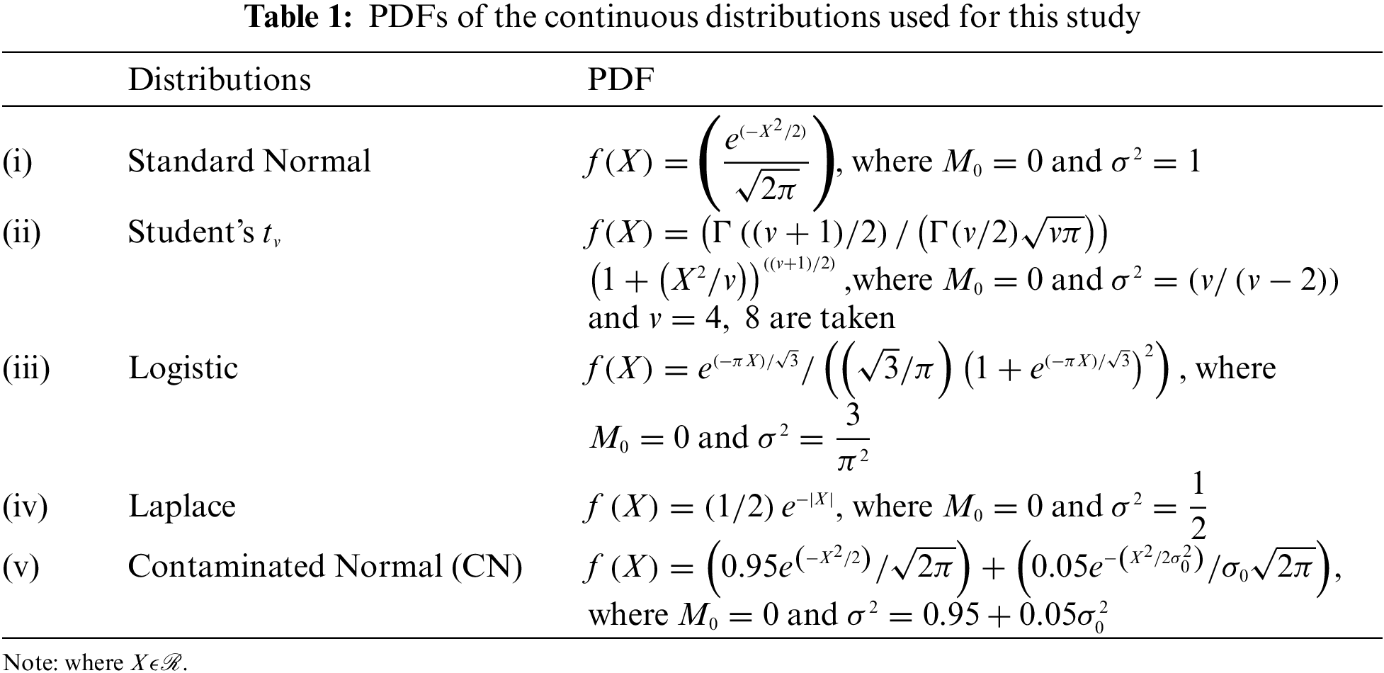
The IC and OOC performances of the proposed NPHWMARSS control chart for monitoring shifts in process location are presented in this section. Generally, we study the RL distribution and its associated features to assess the behavior of the control chart. The average run length (ARL) is the basic metric to evaluate control chart performance. It can be defined as the average number of sample points plotted on the control chart before the control chart shows an OOC signal [41]. Mathematically it is defined as ARL=∑i=1NRLi/N, where N is the size of simulation runs (see Almanjahie et al. [42]). For the IC process, the control chart should have large ARL0 to avoid the false alarm, while for the OOC process the ARL1 should be small for early shifts detection. For better performance of the control chart, it is necessary that the ARL1 should be smaller than the other charts at a fixed value of ARL0. In this study, the ARL0 is set on 500, with sample sizes n of 5 and 10. To investigate the performance behavior of the proposed NPHWMARSS chart, various values of η∈ (0.05, 0.10, 0.25, 0.50) and δ∈ (0, 0.025, 0.05, 0.075, 0.10, 0.25, 0.50, 0.75, 1.00, 1.50, 2.00, 2.50, 3.00, 5.00) are used. Sometimes, the researcher may want to examine the chart’s performance across the entire range of shifts, i.e., δmin<δ<δmax. In this case, a variety of performance measures, such as extra quadratic loss (EQL), performance comparison index (PCI), and relative average run length (RARL) can be used. Mathematically, these terms are defined as follows:

(i)   EQL=(δmax−δmin)−1∫δminδmaxσ2ARL(δ)dδ, where ARL(δ) is the ARL at a specific shift (δ) and δmin and δmax represents the minimum and maximum shift values, respectively.

(ii)   PCI=EQL/EQLbenchmark. The PCI value for the benchmark chart is 1, and the PCI value for all other charts is greater than 1.

(iii)   RARL=(δmax−δmin)−1∫δminδmaxARL(δ)ARLbenchmark(δ)dδ, where δmax and δmin are the maximum and minimum shift values, respectively. Also, ARL(δ) and ARLbenchmark(δ) are the ARL values of a given control chart and the benchmark control chart at shift (δ), respectively. A benchmark chart has a lower ARL at a particular point. The RARL value for the benchmark chart is always one. If RARL is greater than one, the benchmark chart is assumed to be superior to the competing chart. It is important to note that the EQL and RARL measures are calculated by numerical integration (trapezoidal) for our study.

Subsection 3.1 offers the IC performance of the proposed NPHWMARSS control chart, while the OOC performance of the proposed control chart is provided in Subsection 3.2.

3.1 IC Performance

This subsection addresses the design and implementation of the proposed NPHWMARSS control chart is given in Subsection 3.1.1. Similarly, Subsection 3.1.2 covers the IC robustness of the proposed NPHWMARSS control chart.

3.1.1 Design and Implementation

The design of the proposed NPHWMARSS control chart is based on the sample size n, smoothing parameter, η, and control chart width L. The combinations of n and η are used to determine the L value so that the ARL0 is approximately equal to its desired value. Further, the extensive Monte Carlo simulations are used to implement the proposed NPHWMARSS control chart. An algorithm is developed in statistical software R to approximate the run length distribution. The RL characteristics are computed with the replicate of size 50,000. The simulation algorithm consists of the steps given as follows:

(i)   Generate a random sample from the underlying distribution.

(ii)   Specify the design parameters, i.e., η and L.

(iii)   Draw a sample from any distribution used in this study.

(iv)   Compute the plotting statistic NPHt in Eq. (12).

(v)   Find LCL(NPHWMARSS)t and UCL(NPHWMARSS)t from Eq. (13).

(vi)   Plot NPHt against LCL(NPHWMARSS)t and UCL(NPHWMARSS)t along t.

(vii)   If NPHt>UCL(NPHWMARSS)t or NPHt<LCL(NPHWMARSS)t, then stop the simulation and calculate the sequence order RL. For instance, at t=235, if NPHt>UCL(NPHWMARSS)t or NPHt<LCL(NPHWMARSS)t, record 235 as a first RL.

(viii)   Repeat Steps (ii) to (vii) 50,000 times and calculate the ARL. Check whether it is desired ARL0; otherwise, adjust constants accordingly in step (ii) and repeat from (ii) to (viii) steps until the desired ARL0 obtained.

(ix)   To compute ARL1 values, draw a shifted sample from the underlying distribution, and repeat Steps (ii) to (ix).

3.1.2 IC Robustness

This Subsection highlights the proposed NPHWMARSS chart’s IC robustness when shifts are reflected in the process location. The various distributions considered for this study, for instance, standard normal distribution, i.e., N(0,1), double exponential or Laplace distribution, i.e., DE(0,12), heavy tail student’s t distribution, i.e., t(υ), logistic distribution i.e., (0,3π), contaminated normal (CN) distribution, which is the mixture of N(0,σ02) and N(0,σ12) (see Table 1). USING NP CONTROL CHARTS, the IC RL distribution and related properties are identical for all continuous and symmetric distributions. Table 2 demonstrates the IC RL characteristics of the proposed NPHWMARSS control chart for monitoring location shifts. These characteristics are computed under normal and non-normal continuous symmetric distributions. The distributions mentioned above are reparametrized to have zero mean/median and unit variance for performance comparison. The analysis indicates that for a specified value of η, the IC RL remains the same for all considered distributions.

3.2 OOC Performance

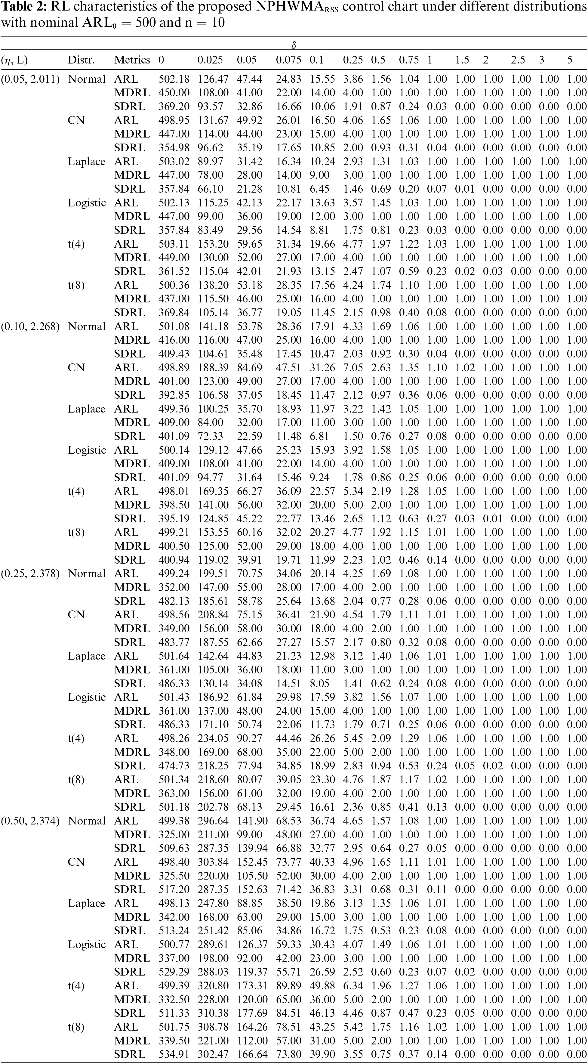
The design parameters of the proposed control chart used to determine OOC efficiency are displayed in Table 2. In order to investigate the OOC performance of the proposed NPHWMA_RSS control chart, numerous values of δ ∈ (0.025, 0.05, 0.075, 0.10, 0.25, 0.50, 0.75, 1.00, 1.50, 2.00, 2.50, 3.00, 5.00) are practiced. The ARL1 measures are used to compare the OOC performance of the proposed and competing control charts.

Table 2, and Figs. 1–3 provide the following outcomes:

(i)   The proposed chart’s IC RL distribution looks similar to all distributions examined in this study (see Table 2).

(ii)   As the smoothing parameter values increase, the performance of the proposed NPHWMARSS control chart deteriorates. (see Fig. 1).

(iii)   As the sample size increases, the shift detection ability of the proposed NPHWMARSS conrol chart enhances. (see Fig. 2).

(iv)   The proposed NPHWMARSS control chart gains better performance under the Laplace distribution than the other distributions (see Fig. 3).

(v)   The proposed chart’s ARL1 values increase as η increases at a certain size of the shift. For instance, under normal distribution at η=0.25,n=10,and δ=0.025, the ARL1=199.51, whereas when η=0.50,n=10,andδ=0.025, the ARL1=296.64 (see Table 2).

(vi)   The RL distribution of the proposed NPHWMARSS control chart is positively skewed, as ARL>MRDL (see Table 2).

(vii)   The efficiency of the proposed control chart with perfect RSS outperforms the efficiency of the proposed control chart with imperfect RSS. For example, with perfect RSS under normal distribution at η=0.10,n=10,and δ=0.025,0.05,0.075,0.1,0.25 the ARL measures are 141.18,53.78,28.36,17.91,4.33 whereas for imperfect RSS at η=0.05,n=10,γ=0.30, δ=0.025,0.05,0.075,0.1,0.25 the ARL measures are 286.98,130.60,75.72,52.80,12.71 (see Table 3). Similarly, with perfect RSS under t-distribution at η=0.10,n=10,and δ=0.025,0.05,0.075 the ARL measures are 153.55,60.16,32.02 whereas for imperfect RSS at η=0.10,n=10,δ=0.025,0.05,0.075 and γ=0.30 the ARL measures are 311.25,155.76,88.89 (see Table 4).

(viii)   The ARL1 values of the proposed NPHWMARSS chart are smaller than competing charts with different shift sizes in process location (see Fig. 4).

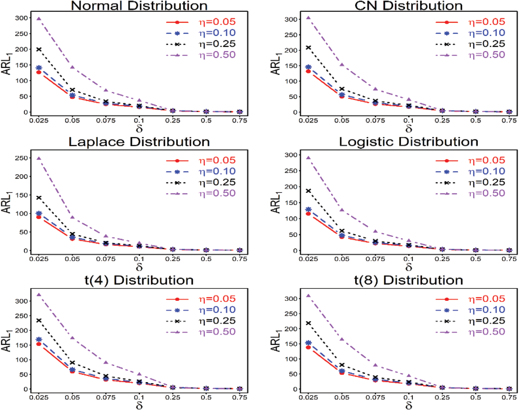
Figure 1: ARL characteristics of the proposed NPHWMARSS control chart for different values of η when n=10 and ARL0=500

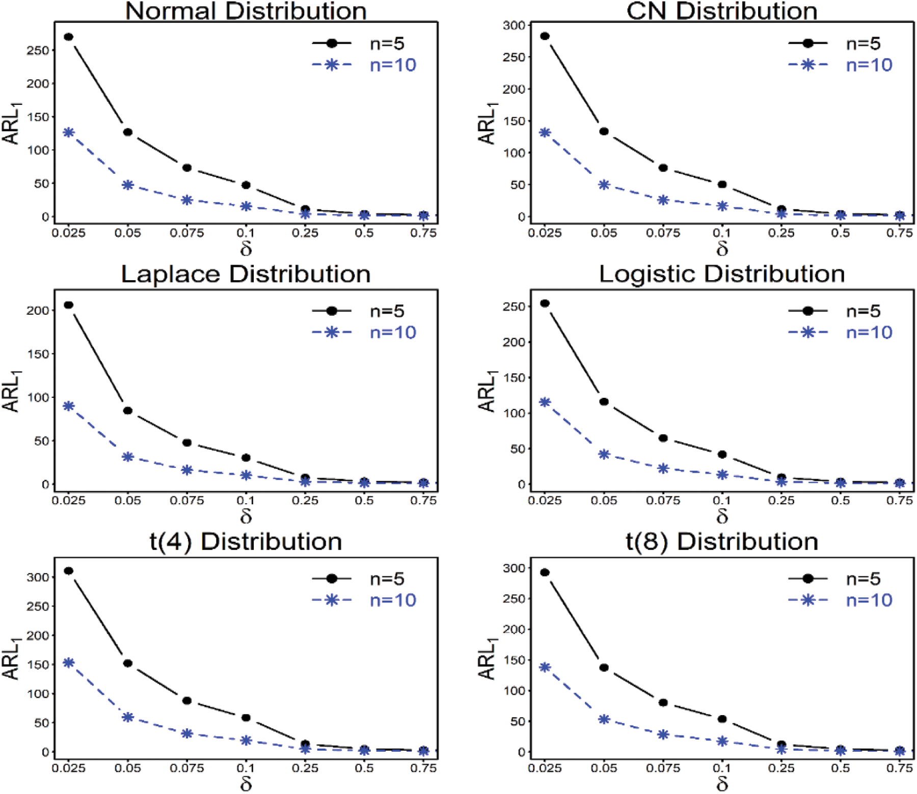
Figure 2: ARL characteristics of the proposed NPHWMARSS control chart when n=5,10 and ARL0=500

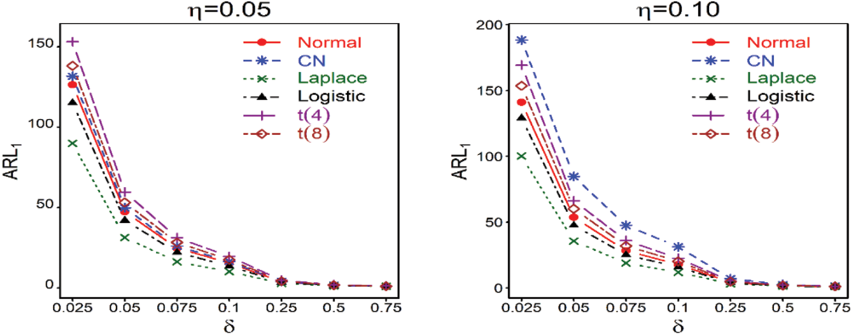
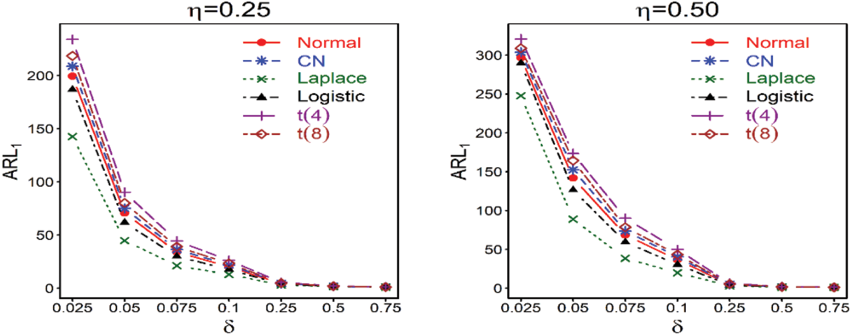
Figure 3: ARL characteristics of the proposed NPHWMARSS control chart under various distributions when n=10 and ARL0=500

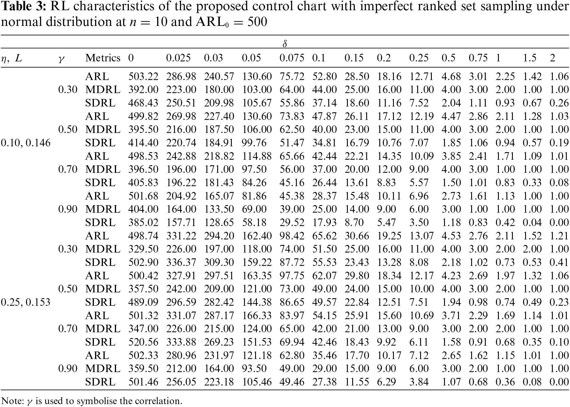
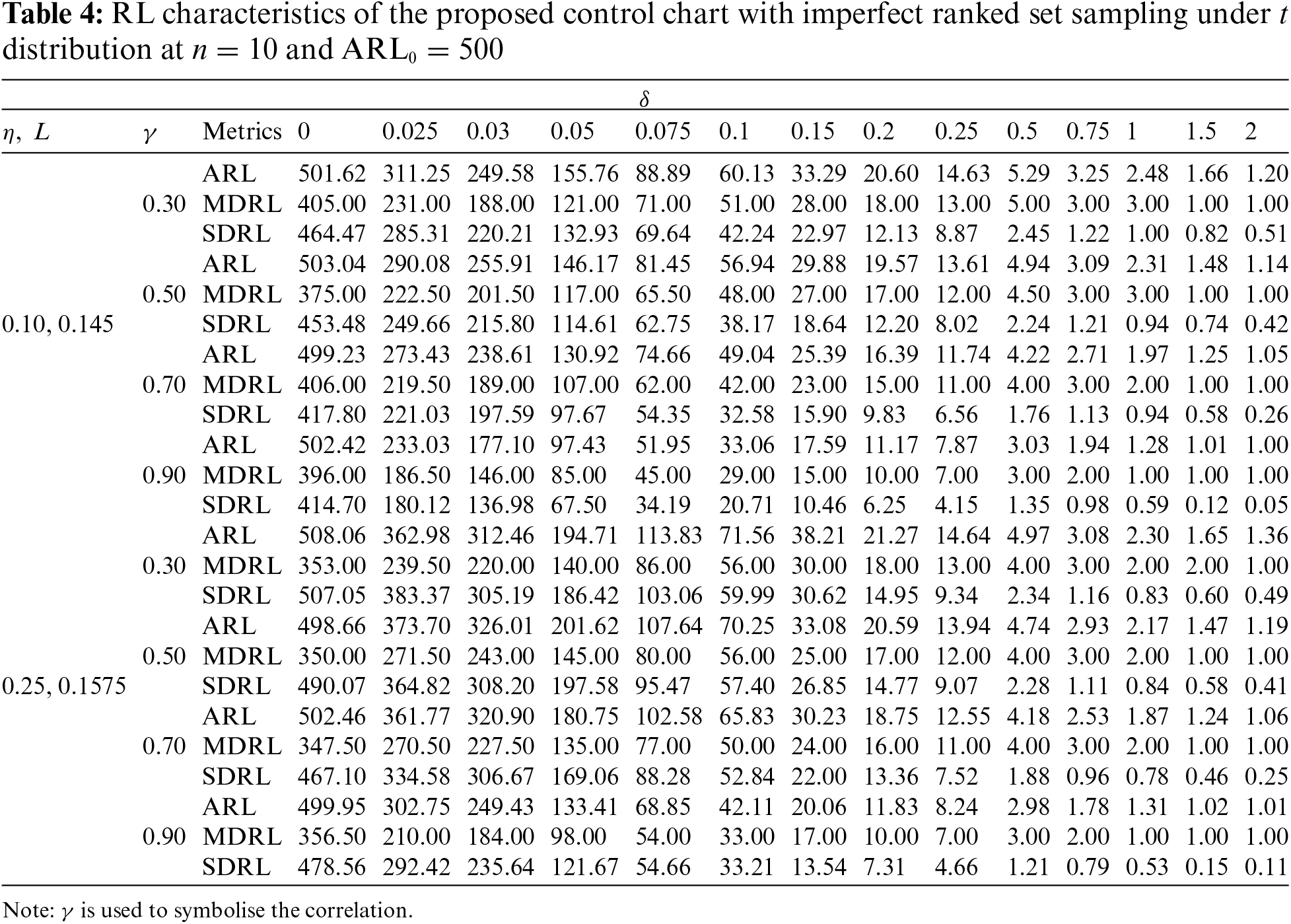
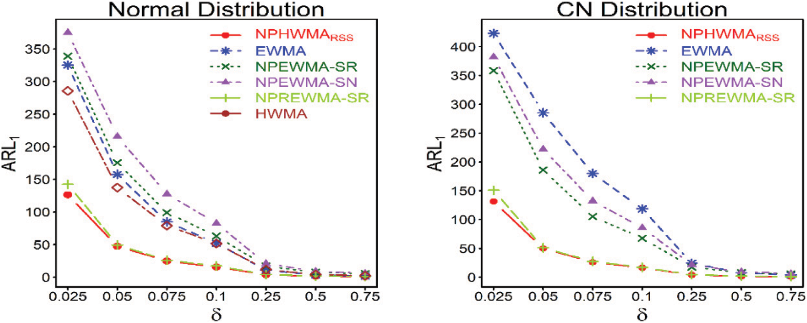
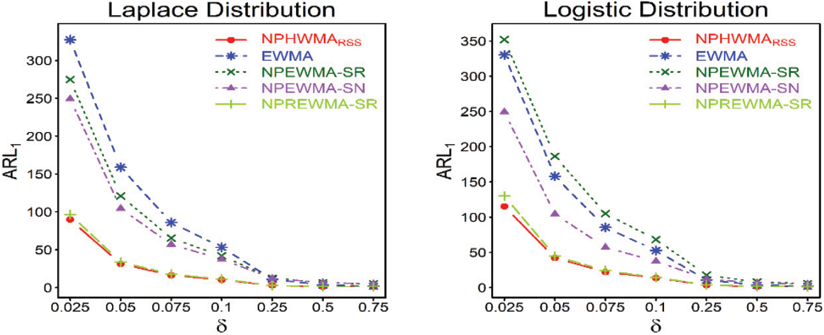
Figure 4: ARL meaures of the proposed NPHWMARSS and competing control charts under various distributions when n=10 and ARL0=500

4  Comparative Study

This section compares the proposed chart against the competing charts, including EWMA, NPEWMA-SR, NPEWMA-SN, NPREWMA-SR, and HWMA control charts. The comparisons are given in the following subsection.

4.1 Proposed vs. EWMA Control Chart

The ARL1 comparison for the proposed NPHWMARSS control chart against the EWMA control chart indicates that the proposed control chart outperforms the EWMA control chart. For example, under normal distribution, when η=0.05,n=10 and δ= 0.025, 0.05, 0.075, 0.10, 0.25, 0.50, 0.75, the ARL1 values of the proposed NPHWMARSS control chart, i.e., 126.47, 47.44, 24.83, 15.55, 3.86, 1.56, 1.04, are smaller than the ARL1 values of the EWMA control chart, i.e., 325.27, 157.51, 84.87, 52.28, 10.93, 3.49, 1.91 (see Tables 2 and 5). Similarly, when we consider Laplace distribution for comparison, we observed the same behavior as the proposed NPHWMARSS control chart.

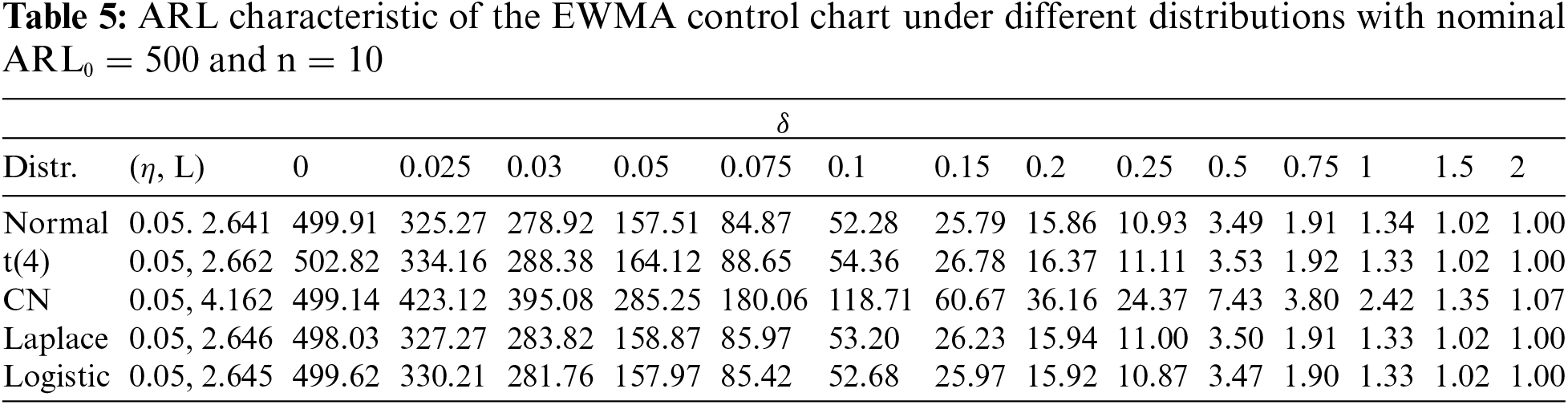
For instance, with the same control chart properties, the proposed NPHWMARSS control chart provides the ARL1 values of 89.97, 31.42, 16.34, 10.24, 2.93, 1.31, 1.03, while the EWMA control chart delivers the ARL1 values of 327.27, 158.87, 85.97, 53.20, 11.00, 3.50, 1.91, respectively (see Tables 2 and 5). Fig. 4 depicts the efficiency of the proposed control chart over the EWMA control chart. Likewise, the proposed NPHWMARSS control chart outperforms the EWMA control chart in terms of overall performance. As an illustration, in the case of normal distribution at η=0.05 the EQL and RARL values of the proposed control chart are 1.41and1.00, while the EQL and RARL values of EWMA control chart are 1.67,1.19 (see Table 6). These findings show that the proposed NPHWMARSS control chart performs better than the EWMA control chart in detecting process location shifts.

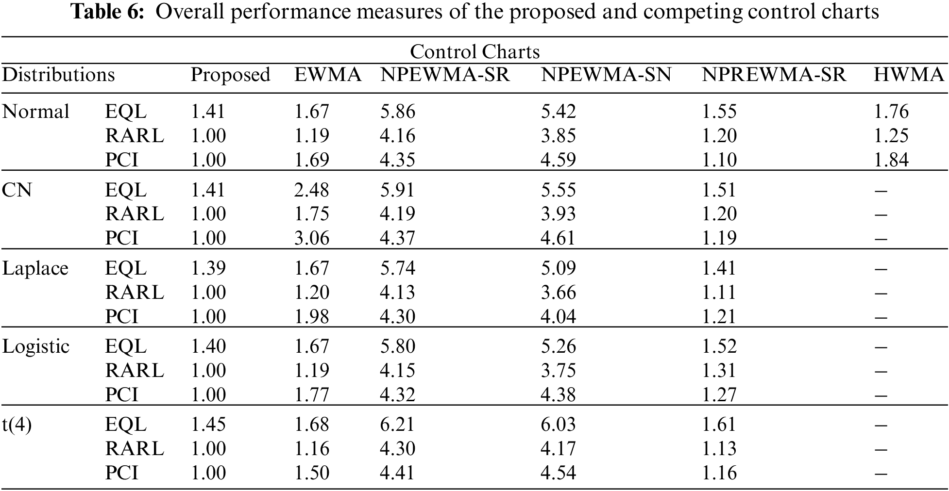
4.2 Proposed vs. NPEWMA-SR Control Chart

In comparison with the NPEWMA-SR control chart, the proposed NPHWMARSS control chart indicates superior performance for all combinations of δ and η. For instance, in case of logistic distribution, when n=10,η=0.05, and δ= 0.025, 0.05, 0.075, 0.10, 0.25, 0.50, 0.75, the proposed NPHWMARSS control chart yields ARL1 values of 115.25, 42.13, 22.17, 13.63, 3.57, 1.45, 1.03, while the NPEWMA-SR control charts has the ARL1 values of 322.05, 158.72, 89.31, 55.32, 15.24, 7.19, 5.20, respectively (see Tables 2 and 7).

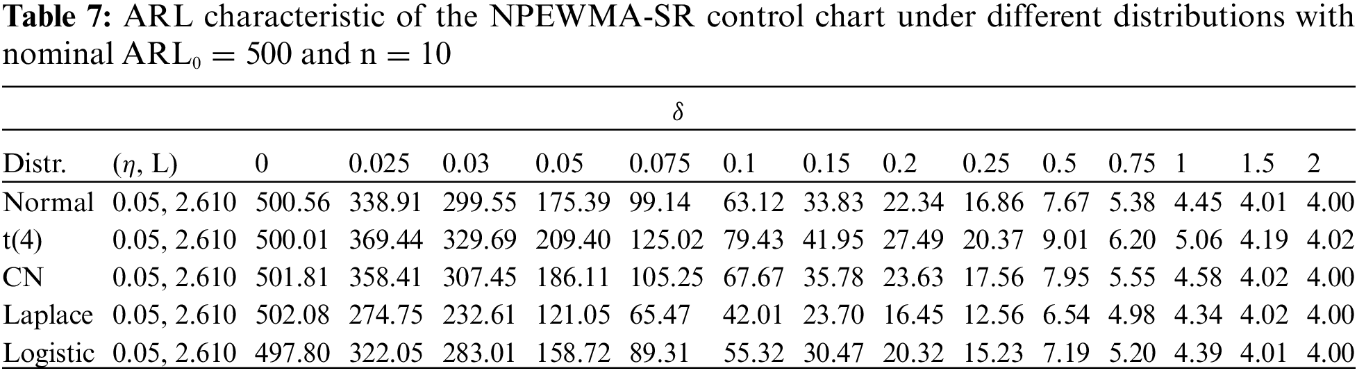
Similarly, when we examine t(4) distribution, with n=10,η=0.05, and δ= 0.025, 0.10 0.25, the ARL1 values of the proposed NPHWMARSS and the NPEWMA-SR control chart are 153.20, 19.66, 4.77, and 369.44, 79.43, and 16.86, respectively (see Tables 2 and 7). Table 6 shows that the PCI performance outperforms the NPEWMA-SR control chart. For example, the proposed control chart has a PCI value of 1.00, whereas the NPEWMA-SR control chart has a PCI value of 4.37 under the CN distribution (see Table 6). The efficiency of the proposed NPHWMARSS control chart to the NPEWMA-SR control chart can also be observed in Fig. 4.

4.3 Proposed vs. NPEWMA-SN Control Chart

The ARL1 comparison reveals that the proposed NPHWMARSS control chart outperforms the NPEWMA-SN control chart for all choices of ηandδ (see Tables 2 and 8). In detail, for CN distribution, with η=0.05,δ=0.075,0.10,0.25, the ARL1 values for the proposed NPHWMARSS control chart are 26.01,16.50,4.06, while for the NPEWMA-SN control chart these values are 132.56,85.70,21.61, respectively (see Tables 2 and 8). Similarly, under normal distribution, at η=5%, a 2.5% increase in process location parameter reduces the ARL by 24.76% for the NPEWMA-SN control chart, while the NPHWMARSS reduces ARL by 74.81% (see Tables 2 and 8). Also, Fig. 4 also shows the superiority of the NPHWMARSS control chart over the NPEWMA-SN control chart. Table 6 shows that the proposed control chart outperforms the NPEWMA-SN control chart in EQL and PCI values under different distributions.

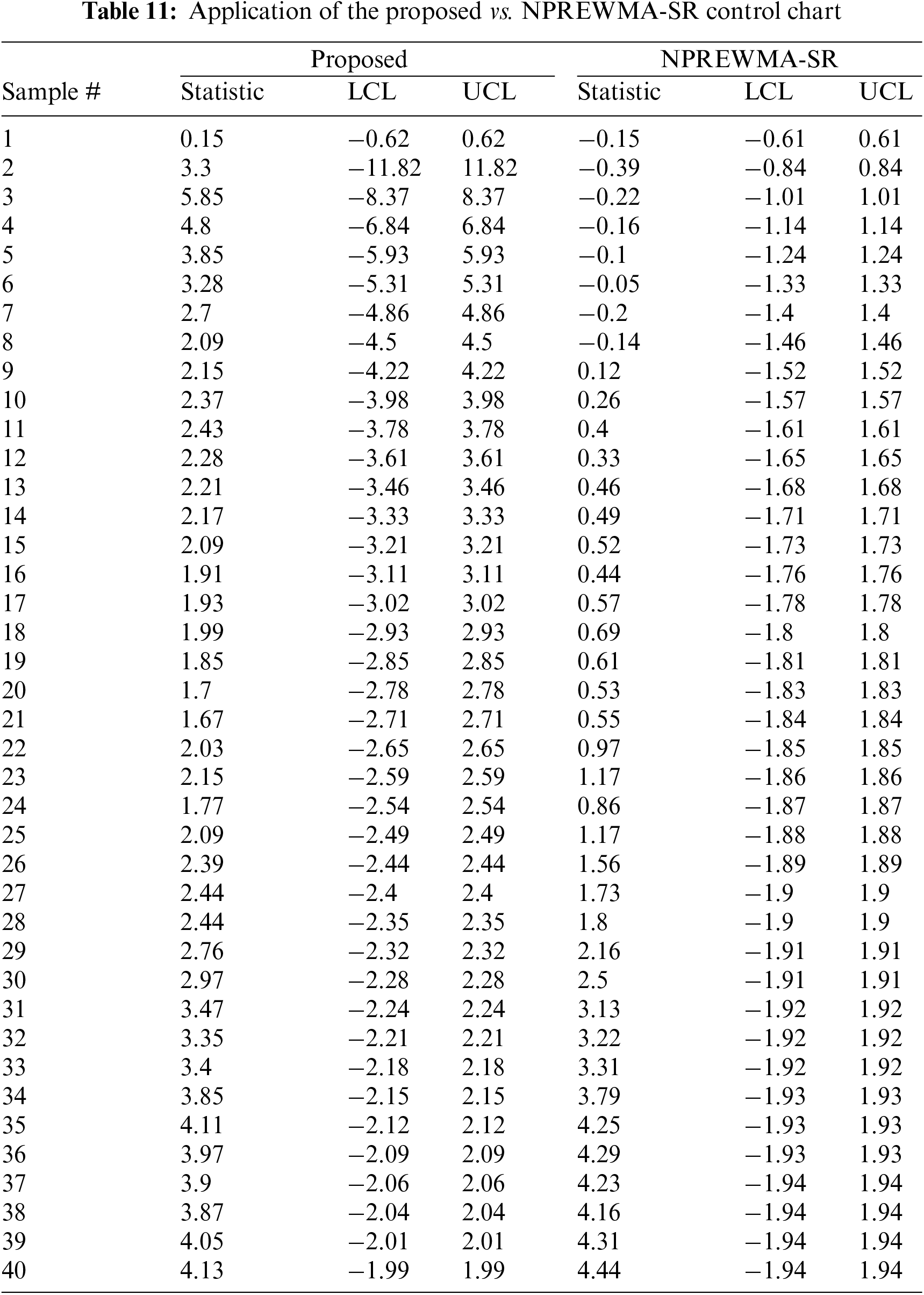
4.4 Proposed vs. NPREWMA-SR Control Chart

The proposed NPHWMARSS control chart performs better than the NPREWMA-SR control chart. For instance, at n=10,η=0.05,δ=0.025, the NPREWMA-SR control chart with Laplace distribution triggers the OOC signal after 94.56 observations, whereas the proposed NPHWMARSS control chart produces the OOC signal after 89.97 observations (see Tables 2 and 9). Similarly, in the case of CN distribution, when n=10,η=0.50andδ= 0.025, 0.05, 0.25, 0.50, then the ARL1 values for the proposed NPHWMARSS control charts are 131.67, 49.92, 4.06, 1.65, whereas the ARL1 values for the NPREWMA-SR control charts are 149.06,51.18,4.67,and1.89, respectively (see Tables 2 and 9 and Fig. 4). Furthermore, under t(8) distribution, at n=10,η=0.05,andδ=0.025,0.05, the OOC ARL for the proposed NPHWMARSS and the NPREWMA-SR control chart are 138.20, 53.18, and 152.17, 54.38, respectively. It is also observed that the proposed control chart outperforms the NPREWMA-SR control chart in terms of overall performance. For example, under Logistic distribution, the RARL value of the proposed control chart is 1.00, while the RARL value of the NPREWMA-SR control chart is 1.31 (see Table 6).

4.5 Proposed vs. HWMA Control Chart

The proposed NPHWMARSS control chart outperformed the HWMA control chart in terms of early shift detection in the process location. For example, investigating the normal distribution with n=10,η=0.10,andδ=0.025,0.05,0.075, the ARL1 values for the proposed NPHWMARSS control chart are observed as; 141.18, 53.78, 28.36, whereas, the ARL1 values for the HWMA control charts are reported as; 307.44, 152.37, 87.46, respectively (see Tables 2 and 10). Similarly, under normal distribution, at n=10,andη=25% reduces the ARL by 124.65% in the HWMA control chart, with a 7.5% increase in the process location parameter, whereas the NPHWMARSS control chart reduces ARL by 34.06% (see Tables 2 and 10). The proposed control chart performs better than the HWMA control chart in terms of overall performance. For example, under normal distribution, the PCI value of the proposed control chart is 1.00, whereas the PCI value of the HWMA control chart is 1.84 (see Table 6). In addition, Fig. 3 illustrates that the proposed NPHWMARSS control chart outperforms the HWMA control chart.

5  Illustrative Example Using Real Data

To demonstrate the applicability of the proposed NPHWMARSS control chart practically, a real-life example is provided in this section. The example used the real-life data of the non-isothermal continuous stirred tank reactor (CSTR) process. This real-life data are considered by numerous authors in their studies, for instance, Lucas et al. [43], Yoon et al. [44], Shi et al. [45], Ridwan et al. [46], and Adegoke et al. [47], etc. The CSTR process has nine variables, one of which we select as the variable of interest (X), representing the output temperature, and this variable is used in real-life application with parameters μX=369.88 and σX2=0.32. The data initially consists of 1000 observations, with the first 500 occurring when the process was in an IC condition. The estimation is carried out with the help of the mentioned parameters, and the control limits are obtained. In order to use the proposed control chart and the existing (NPREWMA-SR) control chart in practise, the variable of interest (X), is used. We used the RSS approach to generate 40 paired observations of size n=5 and m=1 from a normal distribution. After the 24th observation, a shift in the process mean is introduced. The parameters of the proposed and NPREWMA-SR control charts used for real-life analysis are L=2.011,η=0.05,ARL0=500 and L=2.01,η=0.05,ARL0=500, respectively. Fig. 5 indicates that the proposed NPHWMARSS control chart triggers the first OOC signal at sample number 27, while the NPREWMA-SR control chart detects the first OOC point at sample number 29. Similarly, the proposed NPHWMARSS control chart detects overall 14 OOC points, whereas the NPREWMA-SR control chart detects 12 OOC points (see Table 11 and Fig. 5).

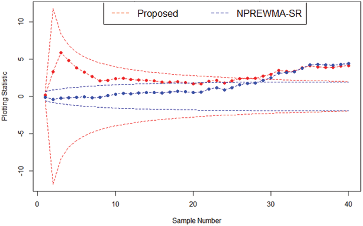
Figure 5: Real-life application of the proposed NPHWMARSS control charts against the NPREWMA-SR control charts

6  Summary, Conclusions, and Future Recommendations

The normality assumption for the process is essential for parametric control charts to monitor process parameters (location and/or dispersion) shifts. If the process under consideration does not follow a normal distribution, the nonparametric (NP) control charts are used. In addition, the homogeneously weighted moving average (HWMA) control chart is introduced for improved process location monitoring. Moreover, the ranked set sampling (RSS) technique outperforms simple random sampling (SRS). This study proposed the NP HWMA control chart with the RSS scheme, which results in an NP HWMA Wilcoxon signed-rank chart under the RSS technique (NPHWMARSS), which is used to improve the shifts detecting ability in the process location. The performance of the proposed chart is examined in terms of ARL,MDRL,and SDRL. The results revealed that the proposed control chart performs better than the competing charts like EWMA, NPEWMA-SR, NPEWMA-SN, NPREWMA-SR, and HWMA. Moreover, a real-life application is also offered to show the proposed control chart’s applicability in practice. The proposed study can be extended to the multivariate scenario.

Acknowledgement: The authors extended their appreciation to the Deanship of Scientific Research at King Khalid University for funding this work through Large Groups Project under the Grant No. RGP.2/132/43. The authors express their gratitude to the editor and referees for their valuable time and efforts on our manuscript.

Funding Statement: Funds are available under the Grant No. RGP.2/132/43 at King Khalid University, Kingdom of Saudi Arabia.

Conflicts of Interest: The authors declare that they have no conflicts of interest to report regarding the present study.

Appendix A

According to Kim et al. [40], for an in control process E(SR(RSS)t)=0 and V(SR(RSS)t)=(r(r+1)(2r+1)6)ϖ02.

A.1.

E(SR¯(RSS)t)=E(1t∑k=1tSR(RSS)k)=1t[ E(SR(RSS)1)+E(SR(RSS)2)+⋯+E(SR(RSS)t) ]=1t[ 0+0+⋯+0 ]=1t[0]=0

A.2.

V(SR¯(RSS)t−1)=V(1t−1∑k=1t−1SR(RSS)k+2∑k<jt−1Cov(SR(RSS)k,SR(RSS)j))

SR(RSS)k and SR(RSS)j are the values from a random sample, so these values are independent of each other. Hence, Covar(SR(RSS)k,SR(RSS)j)=0

V(SR¯(RSS)t−1)=1(t−1)2[V(SR(RSS)1)+V(SR(RSS)2)+⋯+V(SR(RSS)t−1)]=1(t−1)2[(r(r+1)(2r+1)6)ϖ02+(r(r+1)(2r+1)6)ϖ02+⋯+(r(r+1)(2r+1)6)ϖ02]=1(t−1)2[(t−1)(r(r+1)(2r+1)6)ϖ02]=1t−1(r(r+1)(2r+1)6)ϖ02

A.3.

For an in control process Covar(SR(RSS)t,SR¯(RSS)t−1)=0

Covar(SR(RSS)t,SR¯(RSS)t−1)=Covar(SR(RSS)t,SR(RSS)1+SR(RSS)2+⋯+SR(RSS)t−1t−1)=Covar(SR(RSS)t,SR(RSS)1t−1)+Covar(SR(RSS)t,SR(RSS)2t−1)+⋯+Covar(SR(RSS)t,SR(RSS)t−1t−1)=1t−1Covar(SR(RSS)t,SR(RSS)1)+1t−1Covar(SR(RSS)t,SR(RSS)2)+⋯+1t−1Covar(SR(RSS)t,SR(RSS)t−1)=1t−1[Covar(SR(RSS)t,SR(RSS)1)+Covar(SR(RSS)t,SR(RSS)2)+⋯+Covar(SR(RSS)t,SR(RSS)t−1)]

SR(RSS)1,SR(RSS)2,…,SR(RSS)t−1 denotes the first (t−1) samples and all these samples are independent of the next (i.e., tth\right) sample, this implies that

Covar(SR(RSS)t,SR(RSS)1)=Covar(SR(RSS)t,SR(RSS)2)=⋯=Covar(SR(RSS)t,SR(RSS)t−1)=0

Hence

Covar(SR(RSS)t,SR¯(RSS)t−1)=1t−1[0+0+⋯+0]=0

Appendix B

B.1.

The mean of NPHt, i.e., E(NPHt) for an in control process is derived as

E(NPHt)=E(ηSR(RSS)t+(1−η)SR¯(RSS)t−1)=ηE(SR(RSS)t)+(1−η)E(SR¯(RSS)t−1)=η⋅0+(1−η)⋅0=0

E(NPHt)=0

B.2.

The variance of NPHt i.e., V(NPHt) for an in control process is derived as

V(NPHt)=V(ηSR(RSS)t+(1−η)SR¯(RSS)t−1)=η2V(SR(RSS)t)+(1−η)2V(SR¯(RSS)t−1)+η(1−η)Covar(SR(RSS)t,SR¯(RSS)t−1)

V(NPHt)=η2V(SR(RSS)t)+(1−η)2V(SR¯(RSS)t−1)

If t=1 then

V(NPH1)=η2V(SR(RSS)1)+(1−η)2V(SR¯(RSS)0)

As SR¯(RSS)0=0, so

V(NPH1)=η2V(SR(RSS)1)=η2(r(r+1)(2r+1)6)ϖ02

If t>1 then

V(NPHt)=η2V(SR(RSS)t)+(1−η)2V(SR¯(RSS)t−1)=η2(r(r+1)(2r+1)6)ϖ02+(1−η)21t−1(r(r+1)(2r+1)6)ϖ02=(η2+(1−η)2t−1)(r(r+1)(2r+1)6)ϖ02=η2(r(r+1)(2r+1)6)ϖ02+(1−η)21t−1(r(r+1)(2r+1)6)ϖ02=(η2+(1−η)2t−1)(r(r+1)(2r+1)6)ϖ02

References

1. Shewhart, W. A. (1930). Economic control of quality manufactured product. Bell Labs Technical Journal, 9(2), 364–389. [Google Scholar]
2. Page, E. S. (1954). Continuous inspection schemes. Biometrika, 41, 100–115. DOI 10.1093/biomet/41.1-2.100. [Google Scholar] [CrossRef]
3. Roberts, S. (1959). Control chart tests based on geometric moving averages. Technometrics, 1(3), 239–250. DOI 10.1080/00401706.1959.10489860. [Google Scholar] [CrossRef]
4. Yang, S. F., Lin, J. S., Cheng, S. W. (2011). A new nonparametric EWMA sign control chart. Expert Systems with Applications, 38(5), 6239–6243. DOI 10.1016/j.eswa.2010.11.044. [Google Scholar] [CrossRef]
5. Graham, M., Chakraborti, S., Human, S. (2011). A nonparametric EWMA sign chart for location based on individual measurements. Quality Engineering, 23, 227–241. DOI 10.1080/08982112.2011.575745. [Google Scholar] [CrossRef]
6. Graham, M., Chakraborti, S., Human, S. (2011). A nonparametric exponentially weighted moving average signed-rank chart for monitoring location. Computational Statistics & Data Analysis, 55, 2490–2503. DOI 10.1016/j.csda.2011.02.013. [Google Scholar] [CrossRef]
7. Chakraborty, N., Chakraborti, S., Human, S. W., Balakrishnan, N. (2016). A generally weighted moving average signed-rank control chart. Quality and Reliability Engineering International, 32(8), 2835–2845. DOI 10.1002/qre.1968. [Google Scholar] [CrossRef]
8. Abid, M., Nazir, H. Z., Riaz, M., Lin, Z. (2017). An efficient nonparametric EWMA Wilcoxon signed-rank chart for monitoring location. Quality and Reliability Engineering International, 33(3), 669–685. DOI 10.1002/qre.2048. [Google Scholar] [CrossRef]
9. Ali, S., Abbas, Z., Nazir, H. Z., Riaz, M., Zhang, X. et al. (2020). On designing non-parametric EWMA sign chart under ranked set sampling scheme with application to industrial process. Mathematics, 8(9), 1497. DOI 10.3390/math8091497. [Google Scholar] [CrossRef]
10. Lucas, J. M., Saccucci, M. S. (1990). Exponentially weighted moving average control schemes: Properties and enhancements. Technometrics, 32(1), 1–12. DOI 10.1080/00401706.1990.10484583. [Google Scholar] [CrossRef]
11. Shamma, S. E., Shamma, A. K. (1992). Development and evaluation of control charts using double exponentially weighted moving averages. International Journal of Quality and Reliability Management, 9(6), 18–25. DOI 10.1108/02656719210018570. [Google Scholar] [CrossRef]
12. Zhang, L., Chen, G. (2005). An extended EWMA mean chart. Quality Technology and Quantitative Management, 2, 39–52. DOI 10.1080/16843703.2005.11673088. [Google Scholar] [CrossRef]
13. Abbas, N., Riaz, M., Does, R. J. M. M. (2012). Mixed exponentially weighted moving average–cumulative sum charts for process monitoring. Quality and Reliability Engineering International, 29(3), 345–356. DOI 10.1002/qre.1385. [Google Scholar] [CrossRef]
14. Zaman, B., Riaz, M., Abbas, N., Does, R. J. M. M. (2015). Mixed cumulative sum–exponentially weighted moving average control charts: An efficient way of monitoring process location. Quality and Reliability Engineering International, 31, 1407–1421. DOI 10.1002/qre.1678. [Google Scholar] [CrossRef]
15. Anwar, S. M., Aslam, M., Riaz, M., Zaman, B. (2020). On mixed memory control charts based on auxiliary information for efficient process monitoring. Quality and Reliability Engineering International, 36(6), 1949–1968. DOI 10.1002/qre.2667. [Google Scholar] [CrossRef]
16. Adegoke, N. A., Riaz, M., Sanusi, R. A., Smith, A. N., Pawley, M. D. (2017). EWMA-type scheme for monitoring location parameter using auxiliary information. Computers & Industrial Engineering, 114, 114–119. DOI 10.1016/j.cie.2017.10.013. [Google Scholar] [CrossRef]
17. Sanusi, R. A., Riaz, M., Abbas, N. (2017). Combined shewhart CUSUM charts using auxiliary variable. Computers & Industrial Engineering, 105, 329–337. DOI 10.1016/j.cie.2017.01.018. [Google Scholar] [CrossRef]
18. Haq, A. (2018). A new adaptive EWMA control chart using auxiliary information for monitoring the process mean. Communications in Statistics-Theory and Methods, 47(19), 4840–4858. DOI 10.1080/03610926.2018.1448417. [Google Scholar] [CrossRef]
19. Zaman, B., Lee, M. H., Riaz, M., Abujiya, M. R. (2019). An adaptive approach to EWMA dispersion chart using Huber and Tukey functions. Quality and Reliability Engineering International, 35(6), 1542–1581. DOI 10.1002/qre.2460. [Google Scholar] [CrossRef]
20. Aslam, M., Anwar, S. M. (2020). An improved Bayesian modified-EWMA location chart and Its applications in mechanical and sport industry. PLoS One, 15(2), e0229422. DOI 10.1371/journal.pone.0229422. [Google Scholar] [CrossRef]
21. Adeoti, O. A., Malela-Majika, J. C. (2020). Double exponentially weighted moving average control chart with supplementary runs-rules. Quality Technology & Quantitative Management, 17(2), 149–172. DOI 10.1080/16843703.2018.1560603. [Google Scholar] [CrossRef]
22. Abbasi, S., Haq, A. (2019). Optimal CUSUM and adaptive CUSUM charts with auxiliary information for process mean. Journal of Statistical Computation and Simulation, 89(2), 337–361. DOI 10.1080/00949655.2018.1548619. [Google Scholar] [CrossRef]
23. Rasheed, Z., Zhang, H., Anwar, S. M., Zaman, B. (2021). Homogeneously mixed memory charts with application in the substrate production process. Mathematical Problems in Engineering, 2021, 2582210. DOI 10.1155/2021/2582210. [Google Scholar] [CrossRef]
24. Rasheed, Z., Zhang, H., Arslan, M., Zaman, B., Anwar, S. M. et al. (2021b). An efficient robust nonparametric triple EWMA Wilcoxon signed-rank control chart for process location. Mathematical Problems in Engineering, 2570198. DOI 10.1155/2021/2570198. [Google Scholar] [CrossRef]
25. Anwar, S. M., Aslam, M., Zaman, B., Riaz, M. (2021). Mixed memory control chart based on auxiliary information for simultaneously monitoring of process parameters: An application in glass field. Computers & Industrial Engineering, 156, 107284. DOI 10.1016/j.cie.2021.107284. [Google Scholar] [CrossRef]
26. Liu, X., Khan, M., Rasheed, Z., Anwar, S. M., Arslan, M. (2022). New hybrid EWMA charts for efficient process dispersion monitoring with application in automobile industry. Computer Modeling in Engineering & Sciences, 131(2), 1171–1195. DOI 10.32604/cmes.2022.019199. [Google Scholar] [CrossRef]
27. Rasheed, Z., Khan, M., Abiodun, N. L., Anwar, S. M., Khalaf, G. et al. (2022). Improved nonparametric control chart based on ranked set sampling with application of chemical data modelling. Mathematical Problems in Engineering, 2022, 7350204. DOI 10.1155/2022/7350204. [Google Scholar] [CrossRef]
28. Hunter, J. S. (1986). The exponentially weighted moving average. Journal of Quality Technology, 18(1), 203–210. DOI 10.1080/00224065.1986.11979014. [Google Scholar] [CrossRef]
29. Abbas, N. (2018). Homogeneously weighted moving average control chart with an application in substrate manufacturing process. Computers & Industrial Engineering, 120, 460–470. DOI 10.1016/j.cie.2018.05.009. [Google Scholar] [CrossRef]
30. Abid, M., Mei, S., Nazir, H. Z., Riaz, M., Hussain, S. (2020). A mixed HWMA-CUSUM mean chart with an application to manufacturing process. Quality and Reliability Engineering International, 37(2), 618–631. [Google Scholar]
31. Adeoti, O. A., Koleoso, S. O. (2020). A hybrid homogeneously weighted moving average control chart for process monitoring. Quality and Reliability Engineering International, 36(6), 2170–2186. DOI 10.1002/qre.2690. [Google Scholar] [CrossRef]
32. Abid, M., Shabbir, A., Nazir, H. Z., Sherwani, R. A. K., Riaz, M. (2020). A double homogeneously weighted moving average control chart for monitoring of the process mean. Quality and Reliability Engineering International, 36(5), 1513–1527. DOI 10.1002/qre.2641. [Google Scholar] [CrossRef]
33. Anwar, S. M., Aslam, M., Zaman, B., Riaz, M. (2021). An enhanced double homogeneously weighted moving average control chart to monitor process location with application in automobile field. Quality and Reliability Engineering International, 38(1), 174–194. DOI 10.1002/qre.2966. [Google Scholar] [CrossRef]
34. Dell, T. R., Clutter, J. L. (1972). Ranked set sampling theory with order statistics background. Biometrics, 28(2), 545–555. DOI 10.2307/2556166. [Google Scholar] [CrossRef]
35. Bakir, S. T. (2004). A distribution-free Shewhart quality control chart based on signed-ranks. Quality Engineering, 16(4), 613–623. DOI 10.1081/QEN-120038022. [Google Scholar] [CrossRef]
36. Abbas, Z., Nazir, H. Z., Abid, M., Akhtar, N., Riaz, M. (2020). Enhanced nonparametric control charts under simple and ranked set sampling schemes. Transactions of the Institute of Measurement and Control, 42(14), 2744–2759. DOI 10.1177/0142331220931977. [Google Scholar] [CrossRef]
37. Mclntyre, G. A. (1952). A method for unbiased selective sampling using ranked sets. Australian Journal of Agricultural Research, 3(4), 385–390. DOI 10.1071/AR9520385. [Google Scholar] [CrossRef]
38. Takahasi, K., Wakimoto, K. (1968). On unbiased estimates of the population mean based on the sample stratified by means of ordering. Annals of the Institute of Statistical Mathematics, 20(1), 1–31. DOI 10.1007/BF02911622. [Google Scholar] [CrossRef]
39. Stokes, S. L. (1977). Ranked set sampling with concomitant variables. Communications in Statistics-Theory and Methods, 6(12), 1207–1211. DOI 10.1080/03610927708827563. [Google Scholar] [CrossRef]
40. Kim, D. A., Kim, Y. C. (1996). Wilcoxon signed rank test using ranked-set sampling. Korean Journal Computational and Applied Mathematics, 3(2), 235–243. DOI 10.1007/BF03008904. [Google Scholar] [CrossRef]
41. Montgomery, D. C. (2009). Introduction to statistical quality control. New York: John Willey & Sons. [Google Scholar]
42. Almanjahie, I. M., Dar, J. G., Al-Omari, A. I., Mir, A. (2021). Quantile version of Mathai-Haubold entropy of order statistics. Computer Modeling in Engineering & Sciences, 128(3), 907–925. DOI 10.32604/cmes.2021.014896. [Google Scholar] [CrossRef]
43. Lucas, J. M., Crosier, R. B. (1982). Fast initial response for CUSUM quality-control schemes: Give your CUSUM a head start. Technometrics, 24(3), 199–205. DOI 10.1080/00401706.1982.10487759. [Google Scholar] [CrossRef]
44. Yoon, S., MacGregor, J. (2001). Fault dignosis with multivariate statistical models part I: Using steady state fault signatures. Journal of Process Control, 11, 387–400. DOI 10.1016/S0959-1524(00)00008-1. [Google Scholar] [CrossRef]
45. Shi, X., Lv, Y., Fei, Z., Liang, J. (2013). A multivariable statistical process monitoring method based on multiscale analysis and principal curves. International Journal of Innovative Computing, Information and Control, 9, 1781–1800. [Google Scholar]
46. Ridwan, A. S., Muhammad, R., Nurudeen, A. A., Min, X. (2017). An EWMA monitoring scheme with a single auxiliary variable for industrial processes. Computers & Industrial Engineering, 114, 1–10. DOI 10.1016/j.cie.2017.10.001. [Google Scholar] [CrossRef]
47. Adegoke, N. A., Smith, A. N., Anderson, M. J., Sanusi, R. A., Pawley, M. D. (2019). Efficient homogeneously weighted moving average chart for monitoring process mean using an auxiliary variable. IEEE Access, 7, 94021–94032. DOI 10.1109/Access.6287639. [Google Scholar] [CrossRef]