A Deep Learning Approach to Mesh Segmentation

1  Introduction

Automatic segmentation of 3D shapes is an essential phase for geometric modeling and shape processing [1]. It aids in shape comprehension and is at the heart of some computer graphics issues, such as skeleton extraction [2], mesh parameterization, resolution modeling [3], and so on. Several of these applications need to be segmented into more useful parts at a greater level; others, on the other hand, need to be segmented into disk-like fragments at a lower level [4]. As a result, the goal of this paper is to address mesh segmentation using a data-driven strategy. We design a deep network using input mesh training data and the corresponding, intended segmentation to try to understand the trend of segmentation supplied through the training sets to categorize an unknown mesh. As a consequence, we do not, however, make any assumptions about the shape’s geometry or topology nor make use of any descriptors that have been handcrafted.

This paper offers a three-stage method for automatically segmenting a 3D shape into visually recognizable sub-meshes using a deep learning approach, which works well on the Princeton dataset [5]. This is interesting to note that the major goal would be to categorize the 3D mesh rather than perform semantic segmentation. Semantic segmentation assigns the same name wing to an aircraft’s two feathers. The feathers, on the contrary, belong to two separate regions in mesh segmentation and therefore are not labeled in any way. Semantic segmentation, in summary, aids in the comprehension of a 3D model. Mesh segmentation, on the other hand, has significant advantages in mesh processing algorithms such as skeleton extraction [2], mesh parameterization, and resolution modeling [3].

In multi-view segmentation, a 3D shape is created from many views to create multi-view images, which are then fed into a neural network to yield richly labeled images before being converted into to 3D shape. A multi-view segmentation procedure should, in general, solve several technical issues. To begin, there must be sufficient views to reduce occlusions while still encompassing the shape surface. It could be accomplished by producing a huge number of views that are distributed evenly all around the object. Second, shape components could be viewable from multiple perspectives; consequently, the proposed model must efficiently correlate information from various perspectives. One of the fundamental drawbacks of existing multi-view approaches, such as [6,7], is that different views are not connected, resulting in a 3D region with widely varying outcomes from differing perspectives. Furthermore, the view-pooling tactic considers all perspectives evenly, without considering the relationships between them or the discriminative strength of each.

To respond to these challenges, we contend that two essential components are required, to begin, designing the region-to-region connections. If certain aspects of a 3D object are still not explicitly understood from one viewpoint, for instance, (slightly occluded, reflective, and insufficient), other points of view can provide the missing details. When there is a tactic for pairing the areas within a particular view image and the corresponding areas in other viewpoints, the data of that given view could be reaffirmed by utilizing the connections among pairing areas. Furthermore, create a model of the view-to-view connections. When many portions of a 3D object are completely invisible from certain points of view, designing region-to-region connections will not assist some of these views in learning about the invisible parts. To ascertain the discriminatory ability from each perspective, we should design the view-to-view connections and then combine those viewpoints to create the final 3D object and then combine those viewpoints to produce the final 3D object.

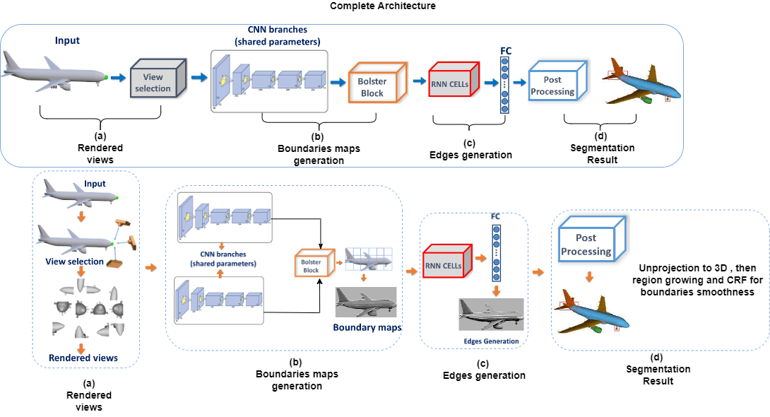
We developed an integrated method for 3D mesh segmentation as a result of the preceding analysis. The general concept of our approach is depicted in Fig. 1. The framework uses a three-stage approach and handles the sequential viewpoints in a temporal order. The first stage involves rendering the object into different views. We ran each view through (shared weights) CNN and Bolster block to create a probability boundary map. The Bolster block simulates the area relationships between different views, which helps to improve and refine the data. The feature maps generated are correlated using LSTM and a fully connected layer to return consistent edges, which are then back-projected to the 3D surface and assimilated by a Conditional Random Field (CRF) to produce the final segmentation.

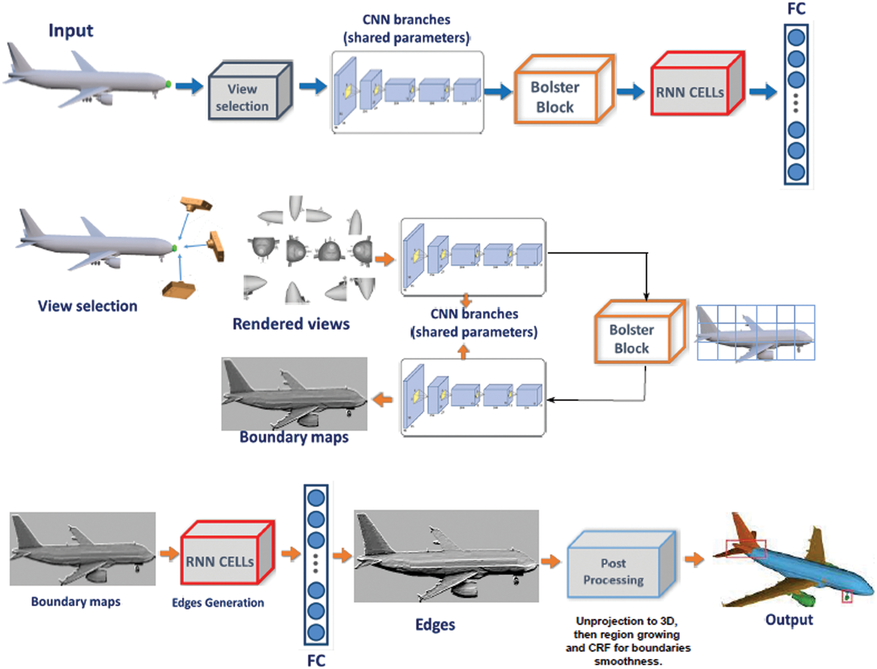
Figure 1: The complete architecture of the presented approach

To address this, we ran each view through (shared weights) CNN and Bolster block to create a probability boundary map. The Bolster block simulates the area relationships between different views, which helps to improve and refine the data. In stage two, the feature maps generated in the previous step are correlated with LSTM to obtain compatible good details responses for every view as well as to obtain the overlap among neighboring viewpoints. Finally, a layer that is connected fully is used to deliver coherent edges, that are projected back to the 3D surface to produce the final segmentation. For instance, on every area in the provided view image, the Bolster block tries to find correlation areas from the other views and strengthens the data of that area by leveraging clues from the corresponding areas. Views can be bolstered in this way. The main contributions of this paper are:

1.    We created an efficient block called the Bolster block. The Bolster block locates correlation areas from other views and strengthens the data of that area by using key information from the corresponding areas for every area inside the given view image.

2.    We propose a network that simulates the area relationships between different views for the task of 3D mesh segmentation. The model employs Long Short-Term Memory layers to generate compatible details responses for every viewpoint as well as the overlap between neighboring viewpoints.

3.    Our model predicts the 3D model’s edges, which is easier for the approach to learn than using large numbers of semantic labels, which is relevant for several other tasks including ridge-valley detection and suggestive contours.

2  Related Work

In this section, we will start by looking at existing handcrafted features and other deep learning methods for 3D mesh segmentation. Then, we discuss Multi-view recurrent neural network and long short-term memory (LSTM) which is used as the recurrent neural unit.

2.1 Hand-Crafted Features

In the field of computer vision and graphics, there is a growing body of literature on handcraft features for 3D mesh segmentation. Such as random walk [8,9], hierarchical clustering [2], region growing [10], k-means [11], spectral clustering [12], normalized cut [13], heat walk [14], and so on. The local characteristics were used to determine the handcraft features to partition a 3D object, like geometric proxies (spheres, cones, etc.), various forms of planarity, and curvatures [15] triangles [16]. A comprehensive review of 3D segmentation techniques is given in [17–19]. In summary, these methods are usually focused on a particular attribute of 3D objects and so are difficult to generalize. Deep learning models benefited from the ability to learn hierarchical discriminative features efficiently.

2.2 3D Deep Learning

Whereas deep learning is commonly used in 2D for more than a decade. Although, unlike photos, 3d models lack fixed structure, Deep learning is used as a method for learning features of high level from lower level features that have been produced in the early stages. The model input segmentation, computation of feature representations, learning of high-level features using auto-encoders, and Graph-Cut segmentation are the steps of an unsupervised shape segmentation approach that was proposed in [20]. For every triangle, local features at various scales are calculated in [21] and are then organize together into a rectangular image, which is then fed back into a network to output the semantic tag for every triangle. Even though these two methodologies employ deep learning methods, they do not fully utilize deep learning’s capability to learn features of high level from low-level features.

Deep learning has received much interest and gained remarkable pragmatic success when combined with appropriate 3D data representations. A thorough overview of 3D data representations can be found in [22]. In this paper, we used mesh as our idle data representation due to its advantages in visualization. This is also why graphics and computer games production companies almost always use polygonal models. Additional 3D shape analysis tasks using 3D mesh data can be found in [23–27]. As a result of the success of deep learning [28,29] and the rapid growth of large 3D archives [30] several solutions for 3D shape analysis tasks were proposed. In general, some of these approaches can be categorized into three main research lines given the input modality: view methods [6,7], voxel methods [31,32], and point methods [33,34].

In voxel approaches, the object is characterized as a 3D occupancy grid, which is subsequently evaluated with neural networks. View approaches render the 3D object from various perspectives and apply image classifiers over each view while the point-based frameworks consider the object to be a muddle of scattered points and generate estimates of the point cloud. Our method is part of the multi-view paradigm, which has in recent times been shown to be capable of a wide range of visual analysis and classification [35]. One of the benefits of view-based methods is that, in comparison to other methods, input views can be easily captured, which is especially useful when access to 3D object models is not possible. Another gain of view-based data is that it is relatively low-dimensional when compared to certain input methods, allowing for more good details regarding the actual 3D object.

Scribble [36] is another deep learning method that proposed a novel weakly-supervised algorithm for segmenting 3D shapes. Their method learns deep neural network parameters while simultaneously propagating information from scribbles to unlabeled faces. As a result, it does not require labeled training shapes and instead relies on a scribble-based partially labeling approach that is relatively easy and convenient. Numerous test results reveal that their proposed method improves earlier unsupervised methods and is comparable to state-of-the-art fully supervised methods in terms of segmentation performance. Shu et al. [37] introduced a unique 3D shape segmentation semi-supervised technique. Using a soft density peak clustering method, users can locate numerous seeds faces with relatively easy interaction. The approach then uses an innovative optimization model to automatically learn the relevant label information and generate satisfactory segmentation results.

Multi-view CNN [6] is the first to use multiple viewpoints together with CNN for the recognition of 3D objects. The 3D shape is rendered in various viewpoints, which are passed through the same image-based CNN. View pooling is used to merge features collected from different views after which it was forwarded via another CNN to obtain the final object label. Xie et al. [35] produced per-view segmentation from depth images using an extreme learning machine as well as merged them using Graph-Cut. Easiness of training an extreme learn algorithm. The above model is often quick to implement. However, the accuracy is still not higher. Kalogerak et al. [38] proposed a much more comprehensive multi-view structure. They begin by rendering the 3D object from various angles which are run through a common CNN before it is unprojected to 3D. A conditional random field is used to rectify the label consistency problem and it’s a network component that is optimized from end to end. Although this method uses the CRF for resolving the consistency problem following 3D un projection, the semantical label pictures were gathered in a max-pooling fashion and are still uncorrelated.

2.3 Recurrent Neural Network

Recurrent neural networks (RNNs) are now successfully used in a number of time series data processing frameworks when working with time-series data, as proposed by [39]. The RNN design is made up of three distinct layers with different timelines that consists of the recurrent layer, the input word layer, and the output layer. A multi-view RNN architecture for generating captions for visual images was proposed in [40].

The multi-view RNN is composed of three subnetworks which are, a network for vision, a network for language, and a network for multiple points of view. Primarily, the network for vision typically employs a deep CNN, like Alexnet, Inception, or Resnet, intending to map an image’s visual information into its representation of deep features. The network for the language takes the representation for the task-specific as well as the temporal dependency. The multi-view network discovers the correlation between language learned and the visual representation using a hidden network. Having followed [40,41] developed a Multiview alignment system based on RNN to connect the inter-view relation among textual and visual data.

An RNN is made up of extremely similar feed-forward neural networks, per each instant or step in times that are known as RNN cells. Many such cells are composed because they function with their output. They also can work with external data to obtain the external outcome, based mostly on RNN cells used, such as Vanilla RNN, LSTM, and so on. Vanilla RNN, despite being efficient and fast, has a few drawbacks. First, it’s hard to make use of post-information if it is changing constantly, as a result, the problem of degenerative changes arises. Furthermore, since Vanilla RNNs are trained using the over-time algorithm back-propagation, vanishing gradient, as well as bursting, seem to be frequent.

The long short-term memory (LSTM) unit [42] was proposed to address the shortcomings of Vanilla RNN and guarantee data integrity. LSTMs also employ gates as a tool for managing and arranging writing, i.e., selectively written, read, and forgotten information is stored in the cell memory. Image segmentation [43], video description [44], and 3D object reconstruction [45], aircraft Operational Loads Monitoring [46], Aerodynamic Modeling [47] are all examples of how LSTMs have been utilized.

3  The Proposed Method

Our approach builds on computer science subfields on randomized algorithms for graph partitioning. Perhaps the most valuable of this work is the technique by [48], which employs a randomized approach to find an optimal cut of a graph. The central concept is to use repeated edge contractions to produce a great number of randomized cuts and then, among the resulting set, find the smallest cost cut. Our work differs in that we use a deep learning method to simulate the area relationships between different views for the task of 3D mesh segmentation. The model employs Long Short-Term Memory layers to generate compatible details responses for every viewpoint as well as the overlap between neighboring viewpoints.

We now present the proposed method, starting with a discussion of the processing of the view Section 3.1, followed by the introduction of the Bolster block Section 3.2, and subsequently edges generation Section 3.3. Finally, we go over the network structure’s specific organization, as shown in Fig. 1.

3.1 Views Processing

Our goal is to use prior knowledge from a pre-segmented training dataset to segment a 3D mesh into parts. We create a Multi-view recurrent neural network to accomplish this. The network is fed an unordered set of 2D perspective projections (rendered views) of surface neighborhoods that capture local context around any surface point at different scales as input. Due to probable occlusions and the absence of adequate surface parametrization characteristics like isometry and bijectivity, such an input representation may seem non-ideal on a first impression. Initially viewing directions are sampled equally about the object defined by spherical coordinates in the pre-processing stage.

A 3D object defined as a polygonal mesh is used as the data input to our method. We simplify and scale it to accommodate a unit sphere as a pre-processing process. The object is then rendered in K variety of views, which are set to 60 based on our tests. Initially, we use [49] to divide the unit sphere into K areas. These areas are where the cameras are placed. We produce grayscale images with the source of light well behind the camera for each view because CNN is relatively resistant to lighting illumination and select a 128 × 128 image resolution to make the training go faster without having to sacrifice the framework’s total segmentation performance. The shaded images generated are handled using an image-based CNN that is identical.

3.2 Bolster Block

When humans identify a 3D object in the environment from a specific viewpoint, they do so naturally, some portions of the object are commonly obscured, reflected, partial, or completely undetectable to human vision. Therefore, humans will require information from other viewpoints to properly grasp the object. For this reason, how to incorporate knowledge from varied viewpoints remains a critical question. Unfortunately, conventional view-based approaches, in general, are inadequate for solving this problem effectively. They lack a technique for reasoning about the connections between 2D appearances from various perspectives. The technique in [6], for example, employs a view-wise pooling mechanism to combine features from individual views into a global 3D object description. The spatial correlation between 2D appearances from multiple viewpoints is neglected by the view-pooling technique.

As a result, the relevant regions from different perspectives are misaligned, and the data from multiple views cannot be successfully merged. To address these concerns, our method is based on the idea that by integrating correlating areas from differing viewpoints and reasoning regarding their connections, the viewpoints can represent the 3D object more effectively. Therefore, the primary objective for every area in a particular view is to locate its correlating areas in other views.

Let Y represent the 3D object. The view series that describes the 3D object is defined by Y = {Y1, Y2,…, YK}. Here K denotes the total number of views. To acquire features at the region level, for every view Yi, its feature convolutional map Ri∈RP×P×Dr can be considered as P × P vectors feature, all of which correlates to a location in viewpoint Yi as a D_r-dimensional representation:

Ri={ri1,ri2,…,riP2},rij∈RDr(1)

where rij is an area feature which is derived from Yi viewpoint within the view series, the bolster block identifies all potential areas and calculates a scalar Mij,mk using a matching function M between rij and every identified area’s feature rmk, indicating how closely these two areas are related:

Mij,mk=M(rij,rmk)(2)

then, based on their similarity measures with rij, all identified areas strengthen the area feature rij. The information from related regions in different views is used to reinforce the region feature. We acquire area features by using the same image-based CNN and used shaded images to generate per-view boundary maps, which we then correlated to get the consistent edges.

3.3 Edges Generation

The works of [28,50,51] are widely used in numerous visual recognition issues and have also been extended to image semantic segmentation effectively [52,53]. Fully convolutional network (FCN) Long et al. [53], for example, was a success in deep network image semantic segmentation. Convolutions with wide receptive fields substitute fully connected layers in a normal CNN in this method, and with coarse class score maps created by feed forwarding an input image, image segmentation is achieved. Moreover, the network’s upsampling deconvolution is limited to bilinear interpolation, and fine-tuned is done only on the CNN portion. The holistically nested-edge detection [54] model transforms traditional edge detection into a CNN-based task. Because of the benefit of fusing the final edge map from numerous edge maps collected at different sizes, we chose HED as a sub-module for our CNN part. Our multi-scale edge maps are side outputs of a VGG-16 network [55], with shallow edge maps capturing fine details and deeper edge maps capturing more salient edges.

The images generated in the previous step are subjected to the same image-based CNN processing. We used the Holistically-Nested Edge CNN architecture [54] to generate the boundary probability map. The discrepancy of the probability maps is resolved by aggregating them using LSTM layers to provide consistent details responses for every viewpoint. The LSTM network, which considers view sequences as time series, is well-suited for this task. To begin, the boundary maps of the ground truth, as well as the boundary probability maps, are unwrapped to vectors 128 × 128 = 16,384 of this size. Two LSTM layers are used with one placed above the other. While the first layer receives a series of unwrapped sorted edge maps and creates a set of embeddings for the second layer, which will effectively create a set of cohesive border maps. For both peepholes, LSTMs [56], we employ the 1024 hidden unit’s number. The results of the subsequent LSTM are relayed across a layer that is fully connected to convert straight to the dimensional edges image.

4  Experiments and Discussion

The testing analyses and evaluations of the method are presented in this section. We run the segmentation technique through its paces using the challenging Princeton dataset [5]. In Section 4.1, we present the dataset details, thereafter, in Section 4.2; we go through the evaluation metrics. In Section 4.3 and Section 4.4, we present training details and back projection to 3D as well as post-processing. Finally, we discuss the results with current state-of-the-art methods on the Princeton Segmentation Benchmark dataset [5] in Section 4.5.

4.1 Datasets and Evaluation Metrics

Princeton Segmentation Benchmark Dataset [5] is commonly utilized thoroughly in assessing 3D mesh segmentation algorithms. There are 20 objects in each of the 19 object categories in the collection which gives in a sum of 380 models. We choose 4 models for testing and 16 models for training at random for each category. Because each model has several human-generated segmentations, we carefully choose one segmentation from each object category that is the most consistent. By rendering the edges between various segments covered by a 3D object of the same coloring as the environment, the ground truth edge pictures could be readily obtained. To improve the ground truth quality, we employ a polygon offset of OpenGL. Both the CNN modules and the LSTM layers are trained using the ground truth edge data.

4.1.1 Evaluation Metrics

We use four metrics defined by [5] to evaluate our segmentation algorithm, which is Cut Discrepancy, Hamming Distance, Rand Index, and Consistency Error. In all four metrics, a lower value implies a better result.

Cut Discrepancy: The first measure, Cut Discrepancy, adds the distances between points along with the calculated segmentation’s cuts and the ground truth segmentation’s closest cuts, and vice versa. It is a boundary-based technique that calculates the distances across cuts [5]. This metric has the advantage of providing a simple and direct assessment of how well borders align.

Hamming Distance: A second metric, Hamming Distance, is used to compare two segmentation outcomes by measuring the entire region-based difference. Given two mesh segmentation S1 and S2, the fundamental concept is to locate the best corresponding segment in S1 for each segment in S2, then add the set differences. If S2 is regarded as the ground truth, the missing rate Rm and false alarm rate Rf can be calculated using Directional Hamming Distance. Its key benefit is that it is based on establishing correspondences between segments, which helps to provide a more relevant evaluation metric.

Rand Index: Rand Index determines whether two faces are in the same segment in two segmentations or distinct segments in both segmentations. The key benefit of this measure is that it can simulate segment area overlaps without the need to find segment correspondences.

Consistency Error: The Consistency Error attempts to account for layered, hierarchical similarities and discrepancies between segmentations. It consists of Local Consistency Error (LCE) and Global Consistency Error (GCE). GCE and LCE are both symmetric. The distinction is that GCE requires all local refinements to be made in the same direction, but LCE permits refinement to be made in multiple directions in different sections of the 3D model. These measurements have the advantage of accounting for layered, hierarchical variances in segmentations.

4.2 Training Details

All of the tests in the Pytorch environment are run on a standalone GeForce GTX NVIDIA 1650 Super, CUDA10.1, and cuDNNV8 with 16 GB RAM. The CNN module is trained in the first stage. We rotated all 3D models in Sixteen various ways at random. Pair of two images, a boundary map ground truth, and a shade image are fed into the network. The cross-entropy sigmoid loss is utilized. We train for 100,000 iterations using the Adam optimizer with a constant learning rate o10−7 and a 16-batch size. After the CNN module has been trained, it is positioned for the second step of training the Edge Generation module.

A combination of boundary maps and boundary maps ground truth is fed into the LSTM layers. Due to memory constraints, we also employ [5] with a 0.01 starting learning rate and 1 batch size. To produce the final segmentation, the consistent edges are projected back onto a 3D surface shape, preceded by Conditional Random Field (CRF) and region growth. Because a significant number of pixels from various viewpoints are likely to match the same vertices, we choose the highest feedback as the peak value. We assign a boundary probability to each edge of the mesh, which is characterized as the mean of the edge values of the vertex connecting. The above border edges define the boundaries of the segmented areas. As a result, we employ a basic region growth method to generate the initial segmentation, with boundary edges functioning as stoppers and segments defined as a sufficiently sized region.

4.3 Post-Processing

The LSTM network’s edge probability maps are reverse projected onto a 3D surface by applying the pixel-to-vertex data that has been stored. A large number of pixels from several viewpoints likely map to the same vertex, as a result, we use the highest response to be the final value. For every mesh edge, we allocate the edge likelihood, which is characterized as the average of the edge likelihoods of the pair of vertices it connects. Lastly, thresholding is used to generate a binary border edge map. These border edges serve as the segmentation of regions’ borders. To obtain the segmentation, we employ a simple region growing method with the border edges serving as blockers. A segment is defined as a region under a large sufficient area. To avoid projection error, the polygons at the borders were unlabeled. Assume that x is the first label for polygon A, x = 0 if A does not have a label and we used Conditional Random Field (CRF) to propagate labels to them.

4.4 Results Discussion

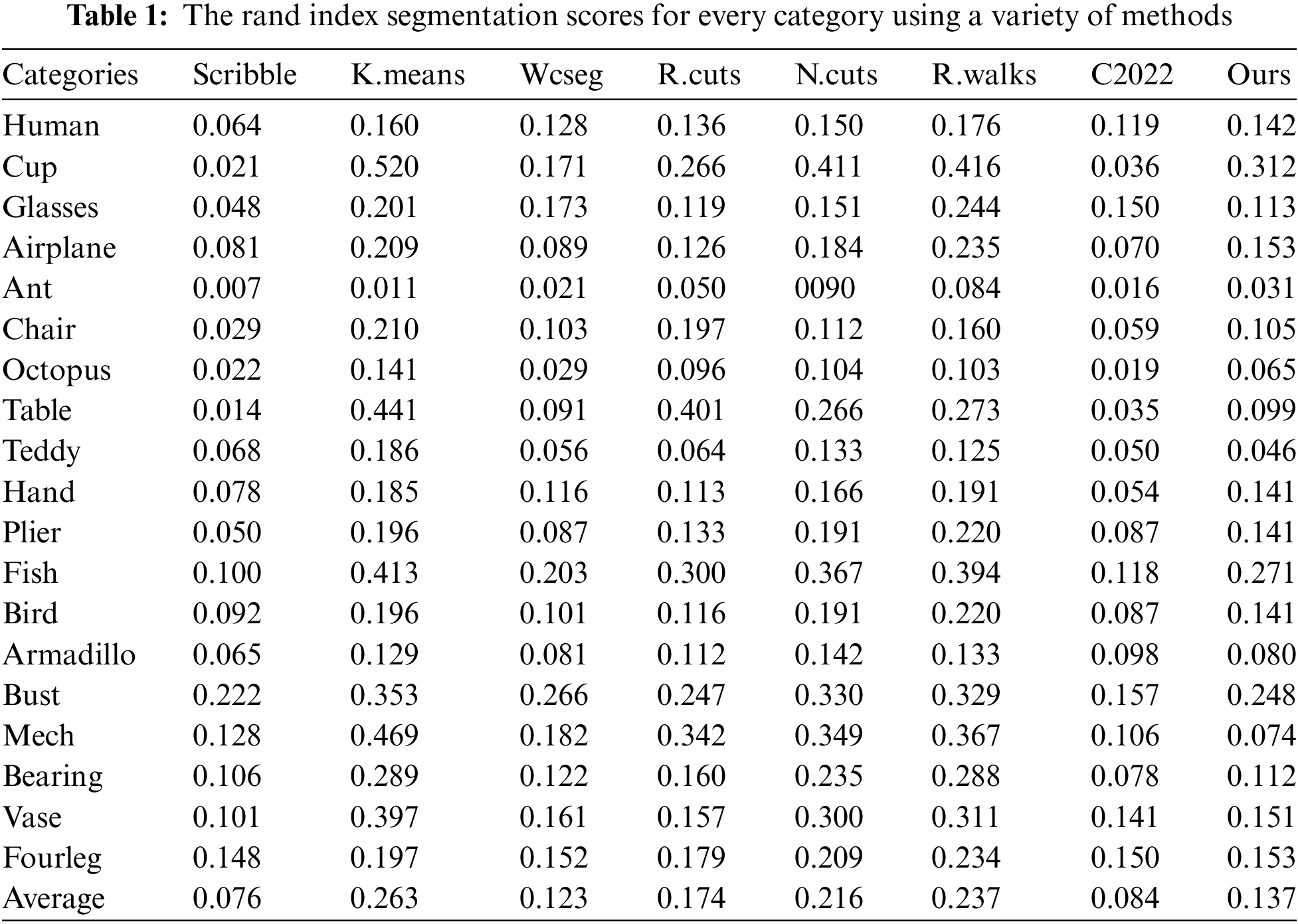
Figs. 2 and 3 show the 2D visualizations of edges for various representative types of 3D meshes from the Princeton dataset. Despite the wide range of shapes, the vast majority of the outputs are desired and consistent. The Rand Index score findings of the segmentation on this dataset, along with other competing techniques, are shown in Table 1. As can be shown, our method achieves an average Rand Index of 0.137, which is comparable to state-of-the-art approaches.

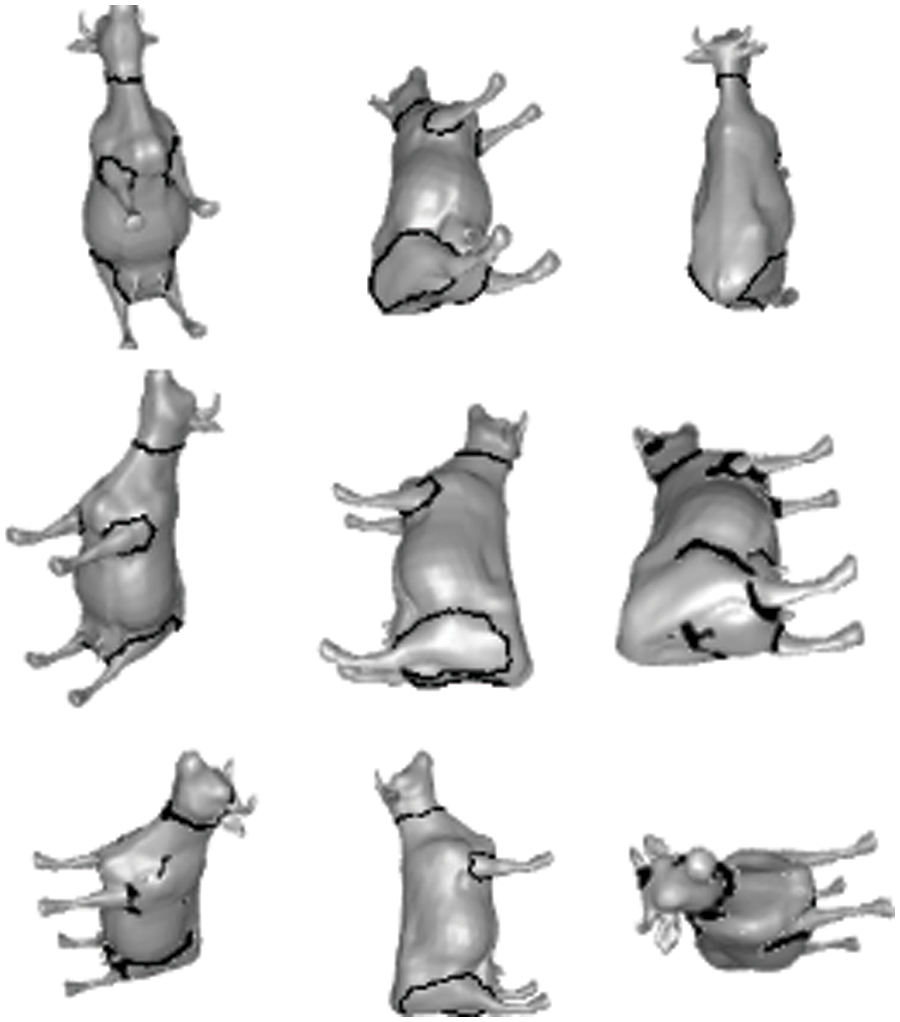
Figure 2: Different views of model 381 edges were obtained using the presented method

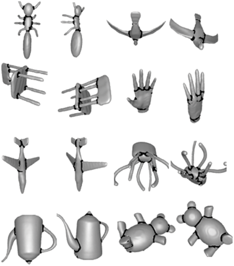
Figure 3: Visualization of the edges generated by our method across different categories on the princeton segmentation dataset

Comparison with previous segmentation algorithms: We compare our method to WcSeg [57], RandCuts [13], Clustering [27], NormCuts [13], RandWalks [8], Scribble [36] and Shu et al. [20] on the PSB dataset. The metrics are used to evaluate the data, and the comprehensive statistics charts are displayed in Fig. 4. The consistency error score of the approach proposed in WcSeg [57] for both GCE and LCE is 0.098 and 0.065, respectively, as shown in Fig. 4, which is lower than our values of 0.088 and 0.064. Figs. 2 and 3 show that our method is capable of precisely identifying the desired borders of 3D shapes. As shown in Fig. 4, our method outperforms [20] in terms of hamming distance, consistency error, and cut discrepancy.

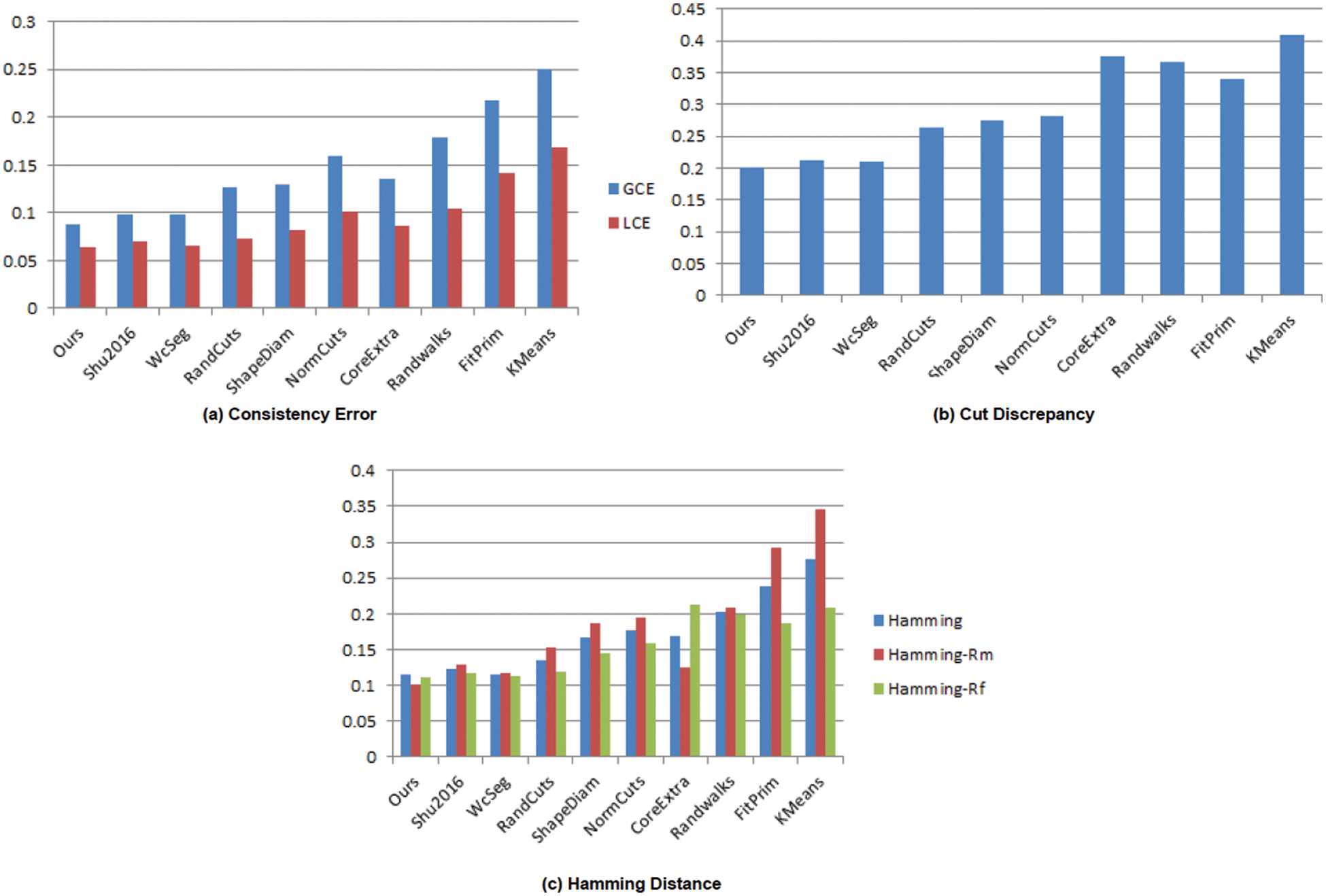
Figure 4: Segmentation algorithms’ performance plots with three assessment metrics. Lower values imply a closer match to the ground truth

Scribble [35] is another deep learning method that we compare our approach with which uses a weakly-supervised algorithm for segmenting 3D shapes. Although the 3D shapes in their training set only include partly labeled data (acquired via scribbles) rather than fully labeled ones, their learning process automatically completely annotates all of the 3D shapes in the training set as a by-product of their algorithm. In certain significant categories, such as mech and teddy, our method outperforms this approach, as shown in Table 1.

We also compared our method to [37], a recent Clustering method. Their method is a two-stage semi-supervised method. They partially tag the training dataset in the first stage using a very simple method that selects clustering centers on the decision graph and trains a neural network model based on the clustering results. The learned neural network model is used to automatically segment the testing 3D shapes in the second stage. The Rand Index Ri, a comprehensive evaluation metric developed by [5], is the major evaluation metric employed in [37]. The Rand Index is a measure of how different the two segmentation outputs are. Table 1 demonstrates that [37] attains an average Rand Index of 0.084, which is slightly above ours with 0.053 but our approach still outperforms this method in some categories such as mech, armadillo, and teddy.

4.5 Comparisons with Randomized Algorithms

Rather than finding a single minimum cut, Rand cuts [13] employ randomized cuts to build a partition function and a set of scored cuts. Randomized algorithms have been utilized by other authors to analyze graphs. For example, randomized repetitions of hierarchical clustering were used by [58] to make several cuts in a graph representing an image, resulting in a similarity function showing the likelihood that two nodes belonged to the same group. By generating cluster centers of the graph produced by leaving edges of likelihood greater than 0.5, the probabilities were utilized to segment the image with “typical” cuts.

For the task of 3D mesh segmentation, we utilize a deep learning method to simulate the area correlations between different viewpoints. This strategy is motivated by two factors. First, previous segmentation methods often include parameters, and differing values for those parameters can drastically vary the set of segments produced. Second, segmentations created by various techniques and parameter settings often cut many of the same edges [59]. As a result, combining the information offered by many discrete segmentations in a probabilistic framework could be beneficial.

We further investigate the qualitative properties of the edges produced by our method. The steps involved in converting the inputs into 2D images, creating the boundary map, and then creating the edges, which are then back-projected to the 3D surface and finally integrated by a CRF, are shown in Fig. 5. The Teddy, Cup, and Chair models are visually compared in Fig. 6 between our approach with Randomized cut and Normal cut. From these examples, we see that our proposed approach successfully generated edges that 1) rest on concave-edged cuts that divide the mesh, 2) focus on cuts that split the mesh into almost equal-sized parts, and 3) do not reside alongside several other desirable cuts.

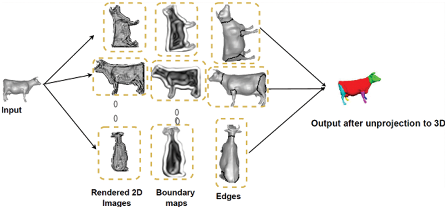
Figure 5: The phases involved in transforming the inputs into 2D images, generating the boundary map, and then the edges, which are then back-projected to the 3D surface and finally integrated by a CRF

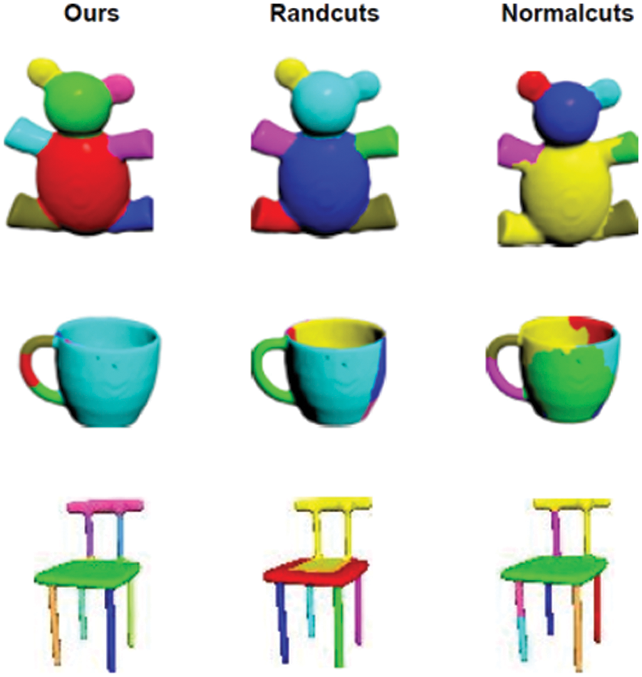
Figure 6: Visual comparison of our approach with randomized cut and normal cut

The first property results from treating numerous views as a temporal sequence and employs RNN to forecast edge images by aggregating the relevant edge probability maps acquired by feed-forwarding the network. The second comes from the LSTM network that correlates these edge maps across different views and outputs a well-defined per-view edge image. The third is a combined result of detecting 3D edges in an end-to-end manner and the segmentation is obtained as post-processing. The processes shown in Fig. 5 show how the inputs are transformed into 2D pictures, the boundary map is produced, followed by the edges, which are then back-projected to the 3D surface and finally integrated by a CRF.

4.6 Ablation Experiment

We alter the number of views and run the experiment with and without LSTM to evaluate the effect of the number of views on the Rand Index and Hamming Distance. As previously stated, the purpose of the LSTM layers is to connect different views and provide consistent edges. The Rand Index is significant because it analyzes two segmentations of the same shape to evaluate how close they are and is mathematically related to accuracy. The relevance of the LSTM block is observed. After removing the block, the network is trained using only the CNN module and all 3D models are rotated in sixteen different ways at random. A pair of images, ground truth from a boundary map, and a shade image are supplied into the network. We train for 100,000 iterations using the Adam optimizer with a constant learning rate of 107 and a 16-batch size. Due to occlusion, using a small number of views is not a viable option, as shown in Fig. 5. Using a larger number of views evenly spread across the whole object, because the surface area of the object is more completely covered, we obtain a greater level of precision (lower Rand Index).

As a suitable trade-off for both effectiveness and latency consumption, we selected 60 views as the number of views. Fig. 7a demonstrates the Rand Index achieved by inserting the LSTM block into the network which results in boosting the Rand Index and Fig. 7b shows the results without the LSTM block. Lower values imply a closer match to the ground truth. We then conducted the experiments for the Hamming Distance using the same setup as our prior Rand Index experiment. The Hamming Distance is a region-based approach that determines how many substitutions are required to transform one region into another. Also, Fig. 8a displays the Hamming Distance obtained by putting the LSTM block into the network, which enhances the Hamming Distance, while Fig. 8b shows the results obtained without the LSTM block, with lower values implying a closer match to the ground truth.

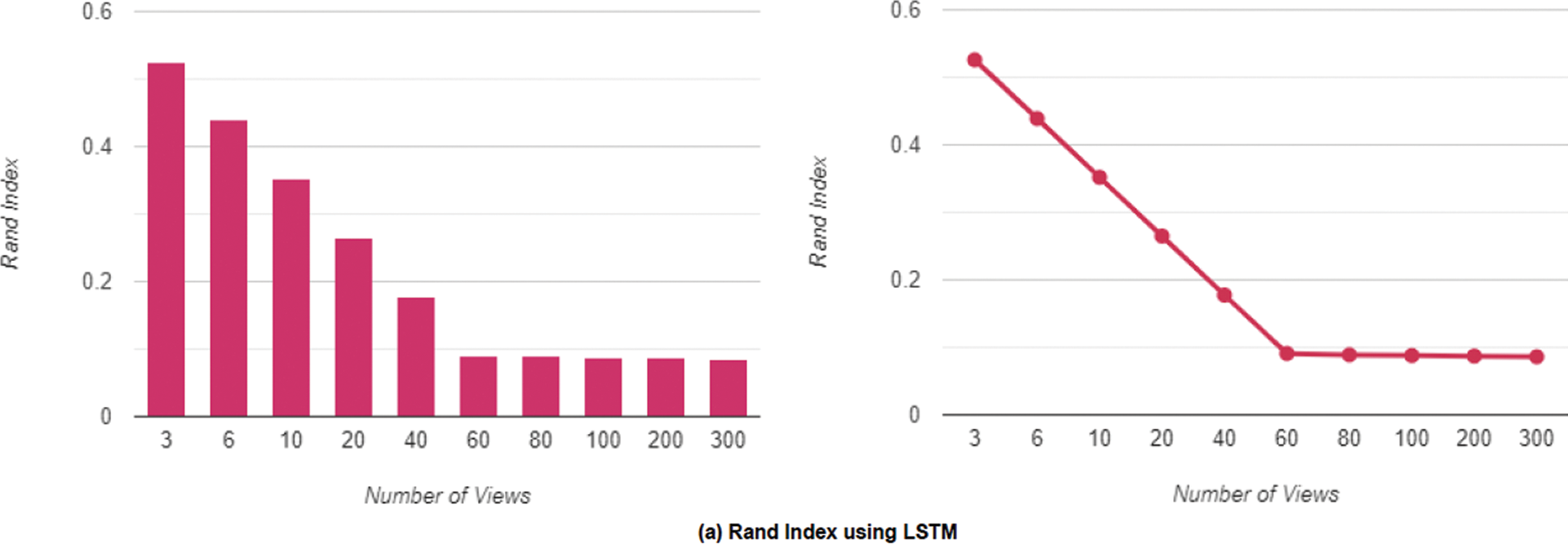
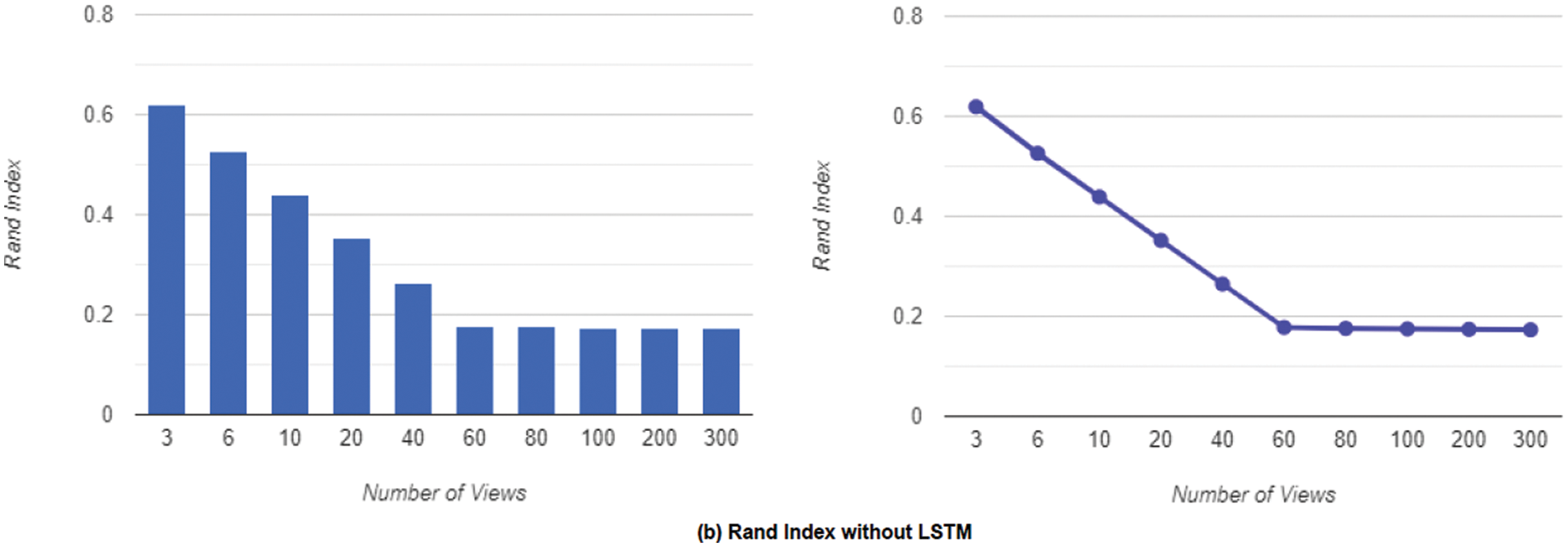
Figure 7: The rand index in terms of the number of views uses 60 as the best trade for both effectiveness and latency consumption

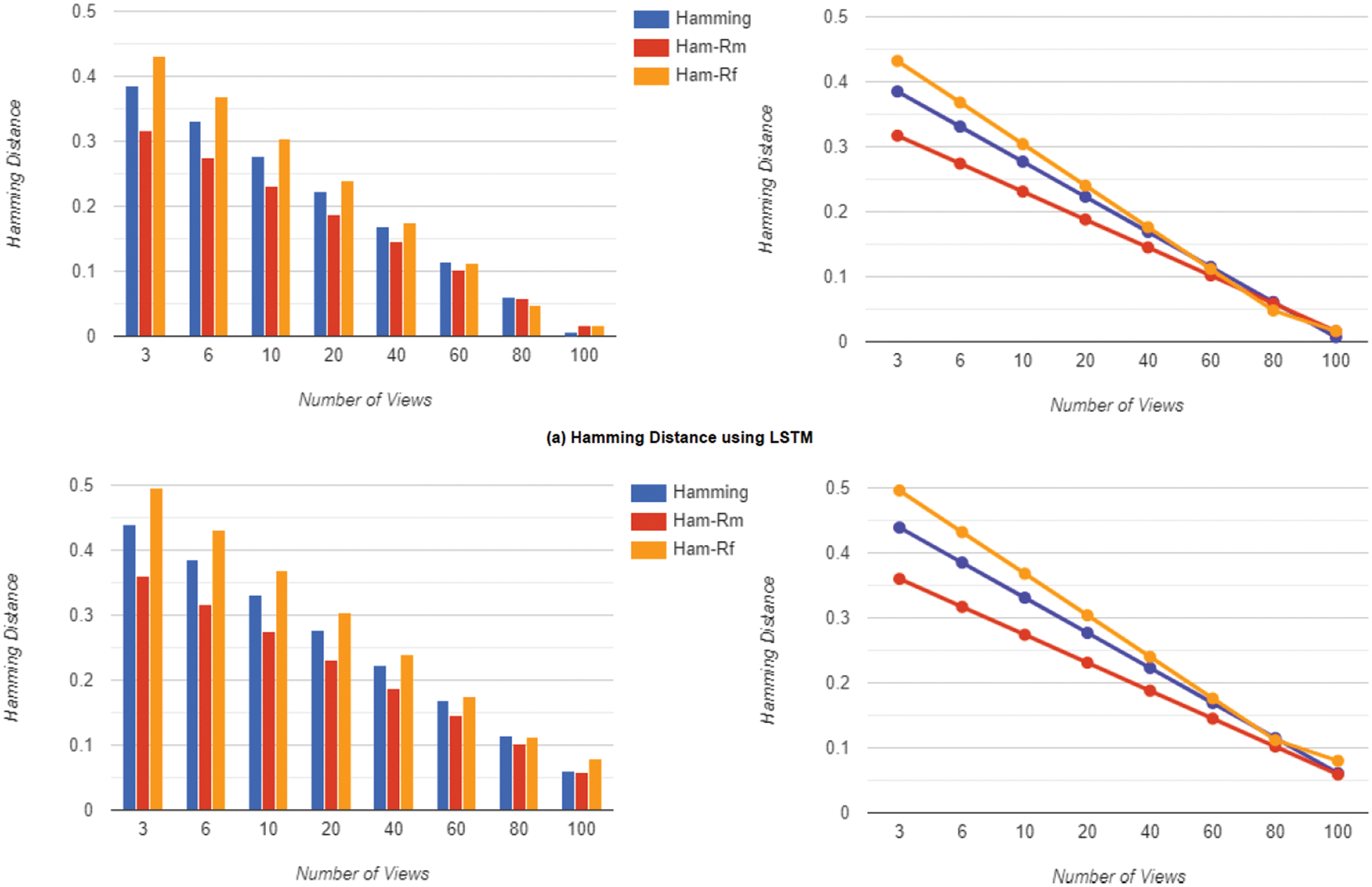
Figure 8: The hamming distance in terms of the number of views using 60 as the best trade for both effectiveness and latency consumption

5  Conclusion

In this paper, a three-stage approach for automatically segmenting a 3D shape into visually meaningful sub-meshes using a deep learning approach is presented. For the task of 3D mesh segmentation, it is necessary to model the area interactions between distinct viewpoints. This is achieved by employing a multi-view network that produces consistent 3D shape segmentation. The proposed system utilizes imaged-based CNN to effectively create the edge feature map and simulates these edge maps throughout other different viewpoints to return consistent edges. Our model predicts the edges of the 3D model, which is easier to train than using a huge number of semantic labels. Edges are valuable for a variety of tasks, including ridge-valley identification, and suggestive contours among others. The presented approach compares favorably to other mesh segmentation algorithms on the Princeton Segmentation Benchmark dataset, according to the experimental results.

Acknowledgement: The authors wish to express their appreciation to the reviewers for their helpful suggestions which greatly improved the presentation of this paper.

Funding Statement: This work was supported by the National Natural Science Foundation of China (61671397).

Conflicts of Interest: The authors declare that they have no conflicts of interest to report regarding the present study.

References

 1.  Wu, Z., Wang, Y., Shou, R., Chen, B., Liu, X. (2013). Unsupervised co-segmentation of 3D shapes via affinity aggregation spectral clustering. Computer & Graphics, 37(6), 628–637. DOI 10.1016/j.cag.2013.05.015. [Google Scholar] [CrossRef]

 2.  Sagi, K., Ayellet, T. (2003). Hierarchical mesh decomposition using fuzzy clustering and cuts. Association for Computing Machinery Transactions on Graphs, 22(3), 954–961. [Google Scholar]

 3.  Funkhouser, T. A., Kazhdan, M. M., Shilane, P., Min, P., Kiefer, W. et al. (2004). Modeling by example. Association for Computing Machinery Transactions on Graphics, 23(3), 652–663. DOI 10.1145/1186562.1015775. [Google Scholar] [CrossRef]

 4.  Garland, M., Willmott, A. J., Heckbert, P. S. (2001). Hierarchical face clustering on polygonal surfaces. Proceedings of the 2001 Symposium on Interactive 3D Graphics, pp. 49–58. New York. [Google Scholar]

 5.  Chen, X., Golovinskiy, A., Funkhouser, T. A. (2009). A benchmark for 3D mesh segmentation. Association for Computing Machinery Transactions on Graphs, 28(3), 12. DOI 10.1145/1576246. [Google Scholar] [CrossRef]

 6.  Su, H., Maji, S., Kalogerakis, E., Learned-Miller, E. G. (2015). Multi-view convolutional neural networks for 3D shape recognition. Proceedings of the IEEE International Conference on Computer Vision (ICCV), pp. 945–953. Santiago. [Google Scholar]

 7.  Wang, C., Pelillo, M., Siddiqi, K. (2017). Dominant set clustering and pooling for multi-view 3D object recognition. arXiv:1906.01592. [Google Scholar]

 8.  Lai, Y., Hu, S., Martin, R. R., Rosin, P. L. (2008). Fast mesh segmentation using random walks. Proceedings of the ACM Symposium on Solid and Physical Modeling, pp. 183–191. New York. [Google Scholar]

 9.  Hou, Y., Zhao, Y., Shan, X. (2021). 3D mesh segmentation via L0-constrained random walks. Multimedia Tools and Application, 80, 24885–24899. DOI 10.1007/s11042-021-10816-0. [Google Scholar] [CrossRef]

10. Vieira, M., Shimada, K. (2005). Surface mesh segmentation and smooth surface extraction through region growing. Computer Aided Geometry Design, 22(8), 771–792. DOI 10.1016/j.cagd.2005.03.006. [Google Scholar] [CrossRef]

11. Yamauchi, H., Lee, S., Lee, Y., Ohtake, Y., Belyaev, A. G. et al. (2005). Feature sensitive mesh segmentation with mean shift. Proceedings of the International Conference on Shape Modeling and Applications, pp. 236–243. Cambridge. [Google Scholar]

12. Shi, J., Malik, J. (1997). Normalized cuts and image segmentation. Proceedings of IEEE Computer Society Conference on Computer Vision and Pattern Recognition, pp. 731–737. Minneapolis. [Google Scholar]

13. Golovinskiy, A., Funkhouser, T. A. (2008). Randomized cuts for 3D mesh analysis. Association for Computing Machinery Transactions on Graphs, 27(5), 145. DOI 10.1145/1457515. [Google Scholar] [CrossRef]

14. Benjamin, W., Polk, A., Vishwanathan, S. V., Ramani, K. (2011). Heat walk: Robust salient segmentation of non-rigid shapes. Computer Graphics Forum, 30(7), 2097–2106. DOI 10.1111/j.1467-8659.2011.02060.x. [Google Scholar] [CrossRef]

15. Lavoué, G., Dupont, F., Baskurt, A. (2005). A new CAD mesh segmentation method based on curvature tensor analysis. Computer Aided Design, 37(10), 975–987. DOI 10.1016/j.cad.2004.09.001. [Google Scholar] [CrossRef]

16. Xiao, D., Lin, H., Xian, C., Gao, S. (2011). CAD mesh model segmentation by clustering. Computer Graphics, 35(3), 685–691. DOI 10.1016/j.cag.2011.03.020. [Google Scholar] [CrossRef]

17. Shamir, A. (2008). A survey on mesh segmentation techniques. Computer Graphics Forum, 27(6), 1539–1556. DOI 10.1111/j.1467-8659.2007.01103.x. [Google Scholar] [CrossRef]

18. Agathos, A., Pratikakis, I., Perantonis, S. J., Sapidis, N., Azariadis, P. N. (2007). 3D mesh segmentation methodologies for CAD applications. Computer-Aided Design and Applications, 4(6), 827–841. DOI 10.1080/16864360.2007.10738515. [Google Scholar] [CrossRef]

19. Theologou, P., Pratikakis, I., Theoharis, T. (2015). A comprehensive overview of methodologies and performance evaluation frameworks in 3D mesh segmentation. Computer Visual Image Understanding, 135, 49–82. DOI 10.1016/j.cviu.2014.12.008. [Google Scholar] [CrossRef]

20. Shu, Z., Qi, C., Xin, S., Hu, C., Wang, L. et al. (2016). Unsupervised 3D shape segmentation and co-segmentation via deep learning. Computer Aided Geometry Design, 43, 39–52. DOI 10.1016/j.cagd.2016.02.015. [Google Scholar] [CrossRef]

21. Guo, K., Zou, D., Chen, X. (2015). 3D mesh labeling via deep convolutional neural networks. Association for Computing Machinery Transactions on Graphics, 35, 1–12. DOI 10.1145/2835487. [Google Scholar] [CrossRef]

22. Gezawa, A. S., Zhang, Y., Wang, Q., Lei, Y. (2020). A review on deep learning approaches for 3D data representations in retrieval and classifications. IEEE Access, 8, 57566–57593. DOI 10.1109/Access.6287639. [Google Scholar] [CrossRef]

23. Wei, X., Chen, Z., Fu, Y., Cui, Z., Zhang, Y. (2021). Deep hybrid self-prior for full 3D mesh generation. Proceedings of the International Conference on Computer Vision (ICCV), pp. 5785–5794. Montreal. [Google Scholar]

24. Suk, J., Haan, P. D., Lippe, P., Brune, C., Wolterink, J. M. (2021). Mesh convolutional neural networks for wall shear stress estimation in 3D artery models. arXiv:2109.04797. [Google Scholar]

25. Wang, N., Zhang, Y., Li, Z., Fu, Y., Yu, H. et al. (2021). Pixel2Mesh: 3D mesh model generation via image-guided deformation. IEEE Transactions on Pattern Analysis and Machine Intelligence, 43, 3600–3613. DOI 10.1109/TPAMI.2020.2984232. [Google Scholar] [CrossRef]

26. Hu, T., Wang, L., Xu, X., Liu, S., Jia, J. (2021). Self-supervised 3D mesh reconstruction from single images. Proceedings of the Conference on Computer Vision and Pattern Recognition (CVPR), pp. 5998–6007. Nashville. [Google Scholar]

27. Fukatsu, Y., Aono, M. (2021). 3D mesh generation by introducing extended attentive normalization. Proceedings of the 8th International Conference on Advanced Informatics: Concepts, Theory and Applications (ICAICTA), pp. 1–6. Yogyakarta. [Google Scholar]

28. Krizhevsky, A., Sutskever, I., Hinton, G. E. (2012). ImageNet classification with deep convolutional neural networks. Communications of the ACM, 60, 84–90. DOI 10.1145/3065386. [Google Scholar] [CrossRef]

29. Ren, S., He, K., Girshick, R. B., Sun, J. (2015). Faster R-CNN: Towards real-time object detection with region proposal networks. IEEE Transactions on Pattern Analysis and Machine Intelligence, 39, 1137–1149. DOI 10.1109/TPAMI.2016.2577031. [Google Scholar] [CrossRef]

30. Chang, A. X., Funkhouser, T. A., Guibas, L. J., Hanrahan, P., Huang, Q. et al. (2015). ShapeNet: An information-rich 3D model repository. arXiv:1512.03012. [Google Scholar]

31. Wu, Z., Song, S., Khosla, A., Yu, F., Zhang, L. et al. (2015). 3D ShapeNets: A deep representation for volumetric shapes. Proceedings of the IEEE Conference on Computer Vision and Pattern Recognition (CVPR), pp. 1912–1920. Boston. [Google Scholar]

32. Li, Y., Pirk, S., Su, H., Qi, C., Guibas, L. J. (2016). FPNN: Field probing neural networks for 3D data. arXiv:1605.06240. [Google Scholar]

33. Qi, C., Su, H., Mo, K., Guibas, L. J. (2017). PointNet: Deep learning on point sets for 3D classification and segmentation. Proceedings of the IEEE Conference on Computer Vision and Pattern Recognition (CVPR), pp. 77–85. Hawaii. [Google Scholar]

34. Qi, C., Yi, L., Su, H., Guibas, L. J. (2017). PointNet++: Deep hierarchical feature learning on point sets in a metric space. Proceedings of the 31st International Conference on Neural Information Processing Systems, pp. 5105–5114. New York. [Google Scholar]

35. Xie, Z., Xu, K., Shan, W., Liu, L., Xiong, Y. et al. (2015). Projective feature learning for 3D shapes with multi-view depth images. Computer Graphics Forum, 34(7), 1–11. DOI 10.1111/cgf.12740. [Google Scholar] [CrossRef]

36. Shu, Z., Shen, X., Xin, S., Chang, Q., Feng, J. et al. (2020). Scribble-based 3D shape segmentation via weakly-supervised learning. IEEE Transactions on Visualization and Computer Graphics, 26(8), 2671–2682. DOI 10.1109/TVCG.2019.2892076. [Google Scholar] [CrossRef]

37. Shu, Z., Yang, S., Wu, H., Xin, S., Pang, C. et al. (2022). 3D shape segmentation using soft density peak clustering and semi-supervised learning. Computer Aided Design, 145, 103181. DOI 10.1016/j.cad.2021.103181. [Google Scholar] [CrossRef]

38. Kalogerakis, E., Averkiou, M., Maji, S., Chaudhuri, S. (2017). 3D shape segmentation with projective convolutional networks. Proceedings of the Conference on Computer Vision and Pattern Recognition (CVPR), pp. 6630–6639. Hawaii. [Google Scholar]

39. Sutskever, I., Martens, J., Hinton, G. E. (2011). Generating text with recurrent neural networks. Proceedings of the 28th International Conference on International Conference on Machine Learning, pp. 1017–1024. Madison, USA. [Google Scholar]

40. Mao, J., Xu, W., Yang, Y., Wang, J., Yuille, A. L. (2015). Deep captioning with multimodal recurrent neural networks (m-RNN). arXiv:1412.6632. [Google Scholar]

41. Karpathy, A., Li, F. (2017). Deep visual-semantic alignments for generating image descriptions. IEEE Transactions on Pattern Analysis and Machine Intelligence, 39, 664–676. DOI 10.1109/TPAMI.2016.2598339. [Google Scholar] [CrossRef]

42. Hochreiter, S., Schmidhuber, J. (1997). Long short-term memory. Neural Computation, 9(8), 1735–1780. DOI 10.1162/neco.1997.9.8.1735. [Google Scholar] [CrossRef]

43. Li, Z., Gan, Y., Liang, X., Yu, Y., Cheng, H. et al. (2016). LSTM-CF: Unifying context modeling and fusion with LSTMs for RGB-D scene labeling. In: Leibe, B., Matas, J., Sebe, N., Welling, M. (Eds.Lecture notes in computer science, vol. 9906, pp. 541–557. Springer, Cham. DOI 10.1007/978-3-319-46475-6_34. [Google Scholar] [CrossRef]

44. Donahue, J., Hendricks, L. A., Rohrbach, M., Venugopalan, S., Guadarrama, S. et al. (2015). Long-term recurrent convolutional networks for visual recognition and description. Proceedings of the IEEE Conference on Computer Vision and Pattern Recognition (CVPR), pp. 2625–2634. Boston. [Google Scholar]

45. Choy, C. B., Xu, D., Gwak, J., Chen, K., Savarese, S. (2016). 3D-R2n2: A unified approach for single and multi-view 3D object reconstruction. European Conference on Computer Vision, pp. 628–644. Amsterdam, The Netherlands. [Google Scholar]

46. Zhou, D., Zhuang, X., Zuo, H., Wang, H., Yan, H. (2020). Deep learning-based approach for civil aircraft hazard identification and prediction. IEEE Access, 8, 103665–103683. DOI 10.1109/Access.6287639. [Google Scholar] [CrossRef]

47. Tekaslan, H. E., Demiroglu, Y., Nikbay, M. (2022). Surrogate unsteady aerodynamic modeling with autoencoders and LSTM networks. AIAA SCITECH 2022 Forum. DOI 10.2514/6.2022-0508. [Google Scholar] [CrossRef]

48. Karger, D. R., Stein, C. (1996). A new approach to the minimum cut problem. Association for Computing Machinery Transactions on Graphics, 43(4), 601–640. DOI 10.1145/234533.234534. [Google Scholar] [CrossRef]

49. Leopardi, P. C. (2006). A partition of the unit sphere into regions of equal area and small diameter. Electronics Transactions on Numerical Analysis, 25, 309–327. [Google Scholar]

50. Szegedy, C., Liu, W., Jia, Y., Sermanet, P., Reed, S. E. et al. (2015). Going deeper with convolutions. Proceedings of the IEEE Conference on Computer Vision and Pattern Recognition (CVPR), pp. 1–9. Boston. [Google Scholar]

51. He, K., Zhang, X., Ren, S., Sun, J. (2016). Deep residual learning for image recognition. Proceedings of the IEEE Conference on Computer Vision and Pattern Recognition (CVPR), pp. 770–778. Las Vegas, USA. [Google Scholar]

52. Farabet, C., Couprie, C., Najman, L., LeCun, Y. (2013). Learning hierarchical features for scene labeling. IEEE Transactions on Pattern Analysis and Machine Intelligence, 35(8), 1915–1929. DOI 10.1109/TPAMI.2012.231. [Google Scholar] [CrossRef]

53. Shelhamer, E., Long, J., Darrell, T. (2017). Fully convolutional networks for semantic segmentation. IEEE Transactions on Pattern Analysis and Machine Intelligence, 39, 640–651. DOI 10.1109/TPAMI.2016.2572683. [Google Scholar] [CrossRef]

54. Xie, S., Tu, Z. (2015). Holistically-nested edge detection. International Journal of Computer Vision, 125, 3–18. DOI 10.1109/ICCV.2015.164. [Google Scholar] [CrossRef]

55. Simonyan, K., Zisserman, A. (2015). Very deep convolutional networks for large-scale image recognition. arXiv:1409.1556. [Google Scholar]

56. Gers, F. A., Schmidhuber, J. (2001). LSTM recurrent networks learn simple context-free and context-sensitive languages. IEEE Transactions on Neural Networks, 12(6), 1333–1340. DOI 10.1109/72.963769. [Google Scholar] [CrossRef]

57. Kaick, O. M., Fish, N., Kleiman, Y., Asafi, S., Cohen-Or, D. (2014). Shape segmentation by approximate convexity analysis. Association for Computing Machinery Transactions on Graphics, 34(1), 1–11. DOI 10.1145/2611811. [Google Scholar] [CrossRef]

58. Gdalyahu, Y., Weinshall, D., Werman, M. (2001). Self-organization in vision: Stochastic clustering for image segmentation, perceptual grouping, and image database organization. IEEE Transactions on Pattern Analysis Machines Intelligence, 23(10), 1053–1074. DOI 10.1109/34.954598. [Google Scholar] [CrossRef]

59. Attene, M., Robbiano, F., Spagnuolo, M., Falcidieno, B. (2007). Semantic annotation of 3D surface meshes based on feature characterization. In: Lecture notes in computer science, vol. 4816, pp. 126–139. DOI 10.1007/978-3-540-77051-0_15. [Google Scholar] [CrossRef]