
 Submit a Paper
 Propose a Special lssue
 Open Access
ARTICLE
Computational Modeling of Reaction-Diffusion COVID-19 Model Having Isolated Compartment
1
Department of Mathematics and Sciences, College of Humanities and Sciences, Prince Sultan University,
Riyadh, 11586, Saudi Arabia
2
Department of Mathematics, Air University, PAF Complex E-9, Islamabad, 44000, Pakistan
* Corresponding Authors: Muhammad Shoaib Arif. Email: ;
(This article belongs to the Special Issue: Recent Developments on Computational Biology-I)
Computer Modeling in Engineering & Sciences 2023, 135(2), 1719-1743. https://doi.org/10.32604/cmes.2022.022235
Received 28 February 2022; Accepted 30 May 2022; Issue published 27 October 2022
 View Full Text
 Download PDF
Abstract
Cases of COVID-19 and its variant omicron are raised all across the world. The most lethal form and effect of COVID-19 are the omicron version, which has been reported in tens of thousands of cases daily in numerous nations. Following WHO (World health organization) records on 30 December 2021, the cases of COVID-19 were found to be maximum for which boarding individuals were found 1,524,266, active, recovered, and discharge were found to be 82,402 and 34,258,778, respectively. While there were 160,989 active cases, 33,614,434 cured cases, 456,386 total deaths, and 605,885,769 total samples tested. So far, 1,438,322,742 individuals have been vaccinated. The coronavirus or COVID-19 is inciting panic for several reasons. It is a new virus that has affected the whole world. Scientists have introduced certain ways to prevent the virus. One can lower the danger of infection by reducing the contact rate with other persons. Avoiding crowded places and social events with many people reduces the chance of one being exposed to the virus. The deadly COVID-19 spreads speedily. It is thought that the upcoming waves of this pandemic will be even more dreadful. Mathematicians have presented several mathematical models to study the pandemic and predict future dangers. The need of the hour is to restrict the mobility to control the infection from spreading. Moreover, separating affected individuals from healthy people is essential to control the infection. We consider the COVID-19 model in which the population is divided into five compartments. The present model presents the population’s diffusion effects on all susceptible, exposed, infected, isolated, and recovered compartments. The reproductive number, which has a key role in the infectious models, is discussed. The equilibrium points and their stability is presented. For numerical simulations, finite difference (FD) schemes like nonstandard finite difference (NSFD), forward in time central in space (FTCS), and Crank Nicolson (CN) schemes are implemented. Some core characteristics of schemes like stability and consistency are calculated.Keywords
In December 2019, the world encountered the most destructive disease named COVID-19. Humankind did not face such crises after World War II, which wreaked great havoc on the nations with the dwindling economies and inadequate health care facilities. It raised the causality rate by 5,534,735 and the fall in trade, movements, and traveling. According to a survey done by international traveling cooperation, about 4 billion people cannot travel due to traveling curbs. This pandemic ceased the government and private medical units as most countries were unprepared and were unaware of the multiplication of causative agents. Today, the coronavirus has produced a new chapter for mathematical researchers who found modeling the most appropriate tool for investigating the spread of a disease in a community.
According to the union health ministry, 653 omicron cases were detected across India in December 2021. However, a dramatic rise has been seen from 29 to 30 December 2021. On 30 December 2021, 13,187 new cases of omicron variant were reported, which were 77% of the total population of India, and the states like Mumbai, Delhi, Pune, Bengaluru, Chennai, Thane, Kolkata, and Ahmedabad were considered as the most susceptible ones. Mumbai showed an 80% rise in the cases daily with an approximation of 2510 cases, leading to a 400% rise weekly. Additionally, 923 cases were detected in New Delhi, which revealed a 600% rise weekly, along with Bengaluru 400 cases (90%), Chennai 294 (100%), and Mumbai (15%). These cases are of the omicron variant, the type of SARS-CoV-2 virus, and have been in destructive action in India since December 2021. The target of vaccination endorse 63% of adults.
The development of vaccines and medicines rectified the pandemic but did not reduce the chance of disease spreading, which has become a great challenge for scientists. This problem can be solved using equilibrium points of COVID-19. People have followed intense SOPs (standard operational procedures) to combat this variant, including quarantine, hand wash, suitable distance, and isolation.
NIH (National Institute of Health) reported that Pakistan had 75 cases since 27 December. Thirty-three were from Karachi, 17 from Islamabad, and 13 from Lahore. Individuals in these cases were found to be international travel. NIH revealed that these patients were immediately isolated and contacted their relatives to control the spread in a statement. On 13 December, The News, the largest-selling paper in Pakistan, coated the figures of NIH and revealed that the first case of omicron was from Karachi.
NIH further stressed the need to follow SOPs and advise people to get vaccinated. The government of Pakistan allowed all the vaccines to be administered as early as possible to get rid of the dire consequences of the omicron variant. NCOC (National Command and Operation Centre) urged people to administer vaccines and booster doses with criteria and precautions. NIH revealed that omicron is a lethal variant whose aftermaths have been multiplying in several countries.
Today, the NCOC issued the latest COVID-19 statistics for the last 24 h in Pakistan, which was 0.69%. Yesterday, 291 new COVID-19 cases were reported while 41,869 diagnostic tests were conducted, whereas three died due to the omicron variant.
Coronavirus was first reported in China city of Wuhan and named COVID-19 by WHO as it shares a common phylogenetic lineage with SARS COVID-II. It is mainly transferred from one person to another due to coughing, sneezing, or contact with infected individuals. Salivary droplets released by infected individuals are denser than air and immediately fall on the ground or nearby. WHO allocated some safety measures, including the distance of six feet, hand washing, wearing masks and gloves, and the quarantining [1,2]. Reportedly, 1,458,000 people were getting infected in more than 180 countries, raising the number of infected individuals by 4 million [3].
A model named as retrofitted state SIR model was proposed by [4] to predict and reckon the numeric of infected and susceptible individuals. Nesteruk focuses on the epidemic and calculates the number of infected individuals. Based on his assumptions, the mortality rate was higher than estimated. Nesteruk et al. [5–8] proved that infection multiplies quickly in densely packed areas, which moves the hypothesis towards applying social distancing and quarantining measures. In [9], authors have investigated the SIR model to estimate the primary cause of coronavirus spread.
Okhuese [10] demonstrated a framework of a stochastic model. The condition dictates extinction and persistence. Also, they debated the threshold of the stochastic model proposed when small or large noise occurs. A method of the potential besides misinformation transmission within the population is the basic reproduction number, mathematically disease-free threshold and stability are related to an epidemic peak and final size [11–15]. The purpose of the present article is to investigate the effects of diffusion on the spread of disease; the reproductive number of the model is given, which is the key element of such models, and the numerical results are obtained through some schemes such as NSFD, FTCS, and Crank Nicolson scheme.
A disease-free equilibrium’s local and global stability is linked to the calculation and epidemiological interpretation of this threshold parameter [16–18]. Following the spread of the disease, researchers have activated to speed innovative diagnostics and are in the throes of several vaccines to guard against COVID-19. Zeb et al. [19] considered the model comprised of five compartments. After the emergency of the acute syndrome coronavirus in 2002, which spread to 37 countries, COVID-19 is the third emerging human application purposes disease in the current century and the middle east respiratory syndrome coronavirus in 2012, which spread to 27 countries bilateral lung infiltration including dry cough, fever, trouble, breathing, fatigue and related symptoms caused by [20–26]. Alqarni et al. [27] constructed a new mathematical model for transmission dynamics of COVID-19. The model is based on the data from Saudi Arabia. The authors have discussed the concentration of the disease by introducing first-order ODE into the model. The whole population is divided into five compartments (
One of the most effective ways to uncover the truth about diseases is through mathematical modeling. For the most part, determining differential equations is difficult and does not yield closed-form solutions. To accomplish this, we turned to a variety of numerical methods.
The detail of the rest of the sections is as follows. The Section 2 discusses the COVID-19 epidemic with an isolated compartment and presented the proposed model. Moreover, we prove the positivity of the model in this section also. The basic reproduction number and equilibrium points are discussed in Section 3. Furthermore, the stability of the equilibrium point is discussed in the same section. In the Section 4, numerical schemes are applied, and the stability and consistency of FTCS, Crank Nicolson, and NSFD schemes are investigated. Sections 5 and 6 are respectively presenting the results and conclusion.
We consider the model for COVID-19, which comprises five compartments susceptible, exposed, infected, isolated, and recovered. The compartments are denoted by
Most infectious disease models comprise ordinary differential equations of the first order. Such models cannot give an accurate picture of disease because of the mobility of the population within the area; therefore, to study pandemic diseases, the spatial content cannot be ignored. Due to the mobility of individuals, the spread of disease may differ from one area to the other.
The movement of people happens in special regions like countries and cities and generally in the local domain. Let’s look at the movement of people in the United States and China (densely populated regions). The mobility of people may be covering millions of square kilometers, whereas, in small countries, it may reduce to just several square kilometers. To what extent does mobility have larger effects on the variation in ecology. This may variate cultural values and health concerns.
Contrary to typical mathematical models, which deal with the spread and control of epidemics, the present model deals with the greater mobility of humans getting mixed rapidly. The specialty of this model is that it keeps the spatial content into consideration. In the case of pandemics, we cannot ignore the factor of mobility because the disease may spread faster in one area than others due to mobility [31–40]. The following flow map in Fig. 1 shows the different compartment SEIQR of the population and the factors affecting the said compartment.
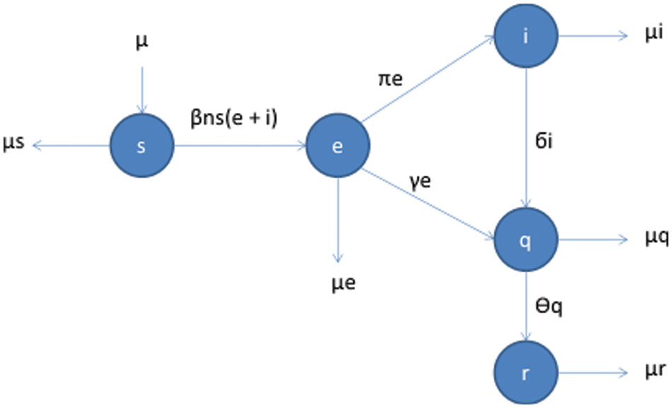
Figure 1: Flow map for COVID-19 model
With initial condition as
As the first four equations are independent of
Consider the following assumptions
With initial conditions
We rewrite the system (3) as follows:
Lemma.1
Under the initial conditions (5), all the solutions of system (6) are non-negative for
Proof: By the I. C.
Eq. (7) proves the positivity of the model.
It is the key element in the disease model whose value is a quick check to tell whether the disease has spread or not. The basic reproductive number for the model is given as
where
2.3 Existence and Stability of Equilibrium Points
Equilibrium points are those critical points that yield a constant solution of differential equations. These points may be stable or unstable depending upon the basic reproductive number
where
2.4 System Stability at Equilibrium Point
For the stability of the system, we perturb (6) at the equilibrium point
where
and
Suppose the above system possesses a Fourier solution
For
This leads to the following:
The variational matrix
The characteristic polynomial for the above matrix can be written as
where
According to Routh Hurwitz’s criterion, the system is stable under the following condition:
Theorem: 1 If
Proof: We construct the Lyapunov function as
This implies that
In this section, we construct numerical methods for system (6).
For
Dividing
We denote the values
The FTCS scheme for the above system can be written as
where
We carry out stability using Von Neumann stability analysis.
Consider the following:
Using the following values:
where
For
After some simplification, we get
Similarly,
For zero linear constants
Now similarly,
For
After some simplification, we have
For
After some Simplification
Therefore, for the system described by (10), the FTCS scheme is conditionally stable.
A finite difference scheme is said to be consistent if the truncation error tends to zero by decreasing the mesh and time step size.
which implies that the FTCS scheme is consistent with the first equation of the system.
Similarly, the same procedure can be used to prove the other equations of the system.
Among finite difference schemes, the Crank Nicolson scheme is one of the best schemes to implement for numerical computation. It gives a better approximation of the solution, which has a temporal error of
Similarly,
where
Also
where
In the same manner, we have the following:
where
3.5 Stability of Crank Nicolson Scheme
We carry out stability analysis using the Von Neumann method.
Consider the following equation of (6).
Here,
For
Similarly, for 2nd equation of the system
Now for 3rd equation of the system
Similarly, Eq. (4) of the system can be written as
Similarly, we can prove the other two equations of the system.
3.6 Consistency of Crank Nicolson Scheme
Consider the following equations:
So, we can proceed as
When
Hence the Crank Nicolson scheme is consistent for the first equation of (6). One can prove other equations of the system in the same way.
Among various numerical techniques used to approximate the differential equations, NFSD is a technique that can effectively be used to approximate differential equations. It holds the property of positivity which is the fundamental property of the pandemic models. Many types of NFSD schemes are formulated according to the rules described by Mickens [17,18].
Consider the following equation of (6).
It can be written as
Similarly, the other equation can be written as
where
We carry out stability analysis using the Von Neumann method. Consider the first equation of system (6)
The discretization of the above equation according to NSFD is as under
where
For
For stability, we must have
Further simplification leads to the following stability condition:
4.2 Consistency of NSFD scheme
The discretization according to NSFD for the first equation of the system can be written as below:
We can write
Therefore,
This leads to the following:
Simplifying further and taking
A similar procedure leads to the consistency of the other equations of the system.
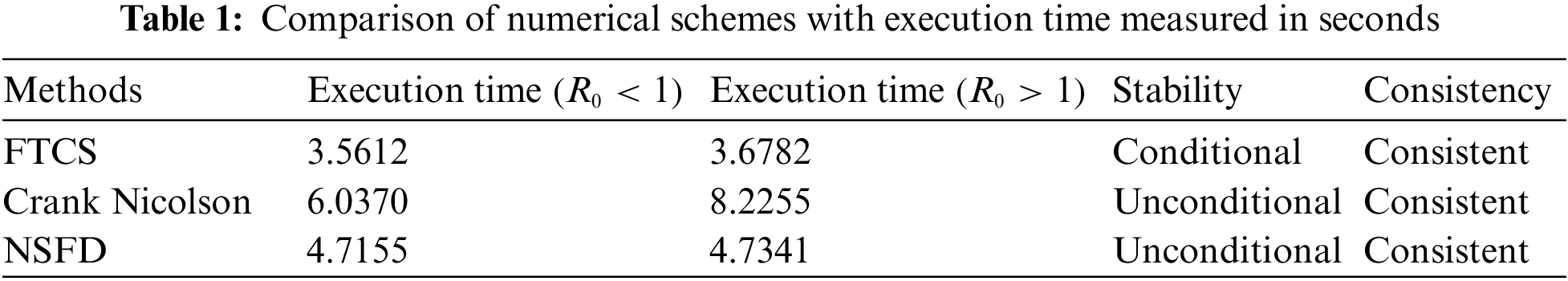
Table 1 compares the schemes applied, with execution time measured in seconds for both cases of Reproductive Number at
For numerical simulations, we have considered two cases depending upon the value of the reproduction number
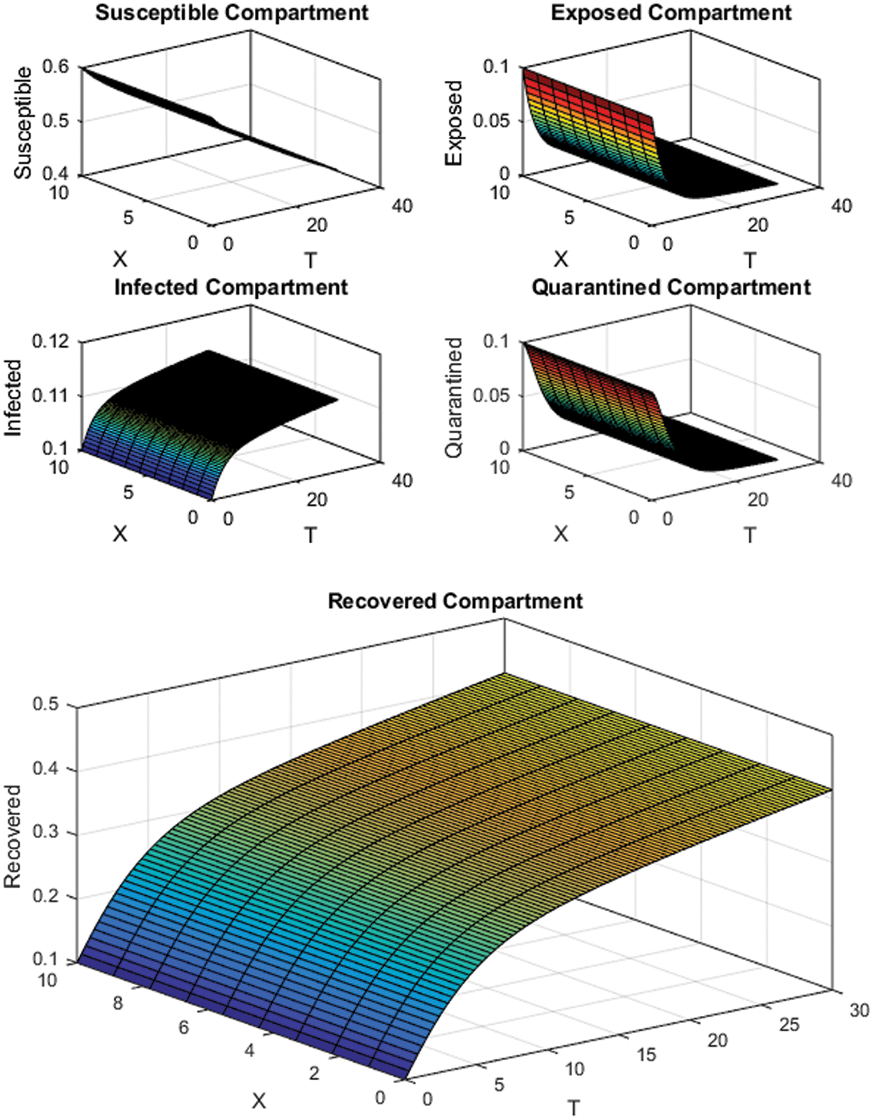
Figure 2: FTCS Scheme with
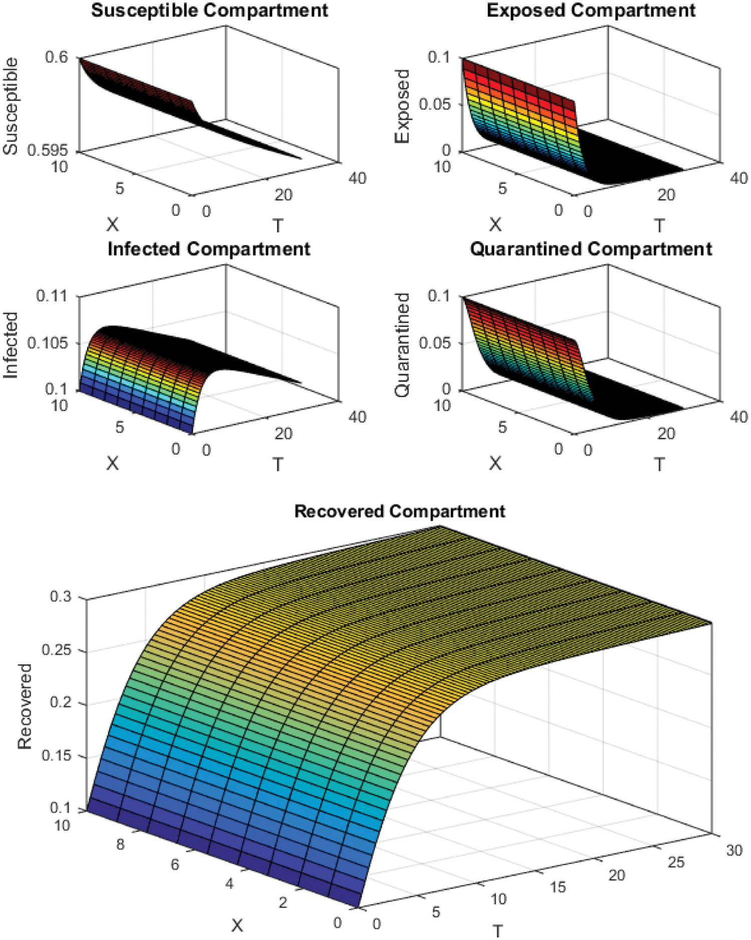
Figure 3: FTCS Scheme with
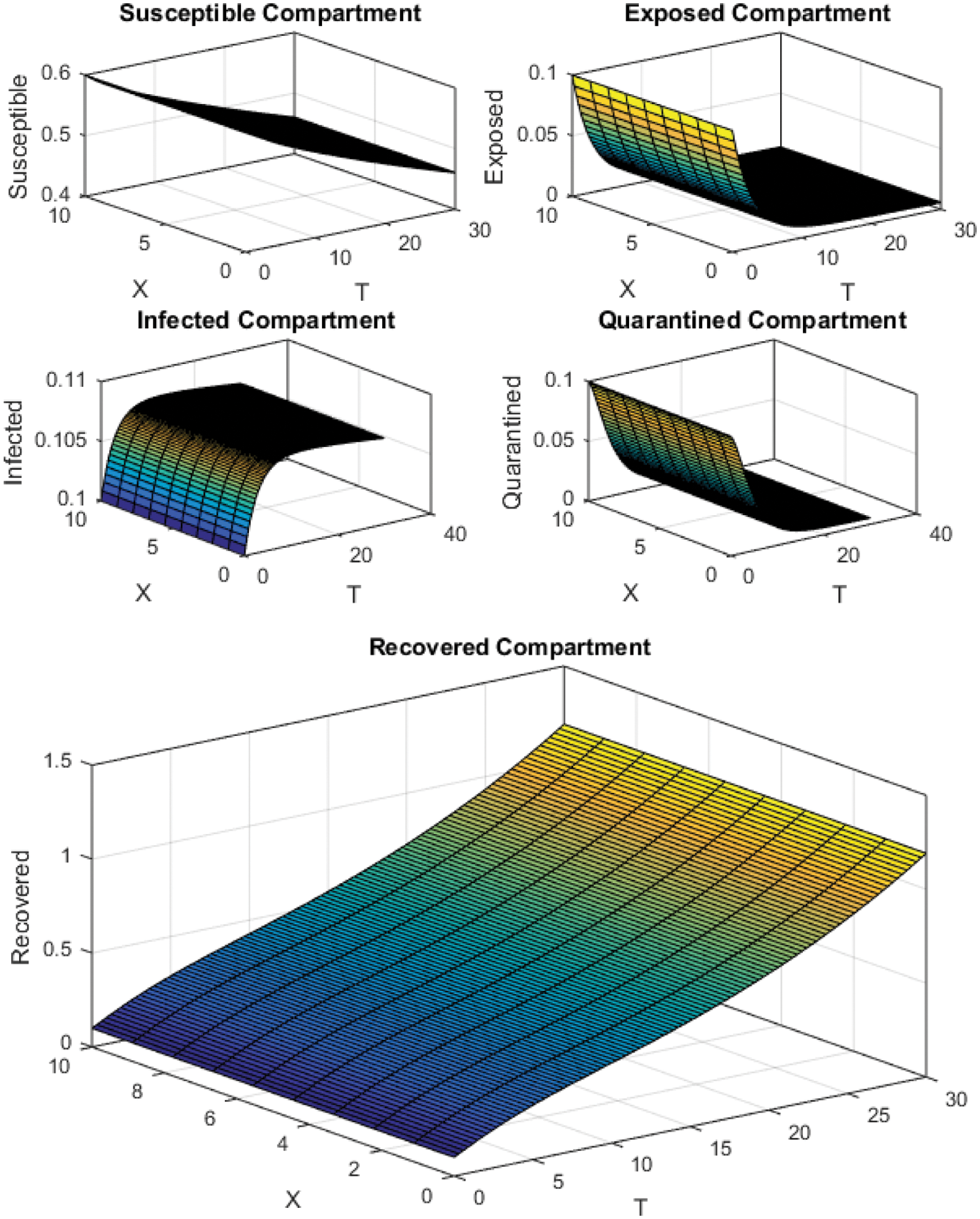
Figure 4: Crank Nicolson Scheme with
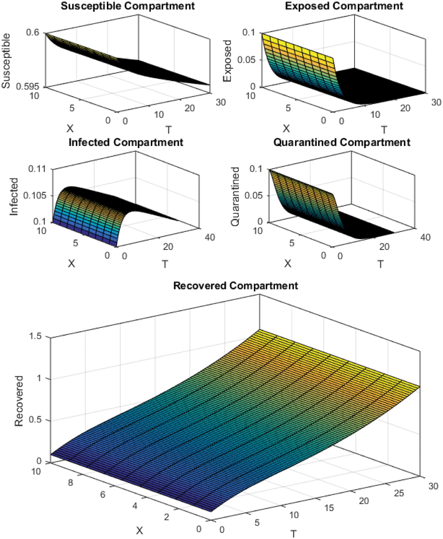
Figure 5: Crank Nicolson Scheme with
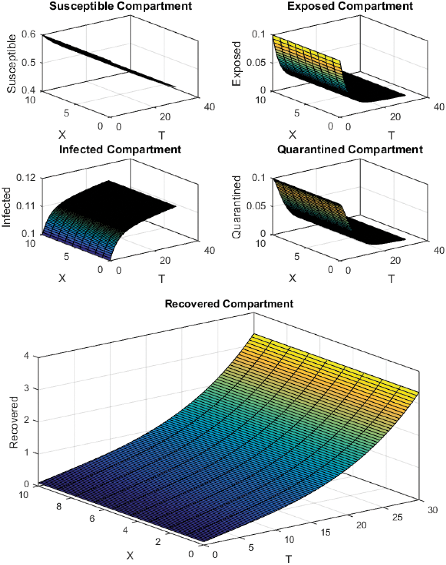
Figure 6: NSFD Scheme with
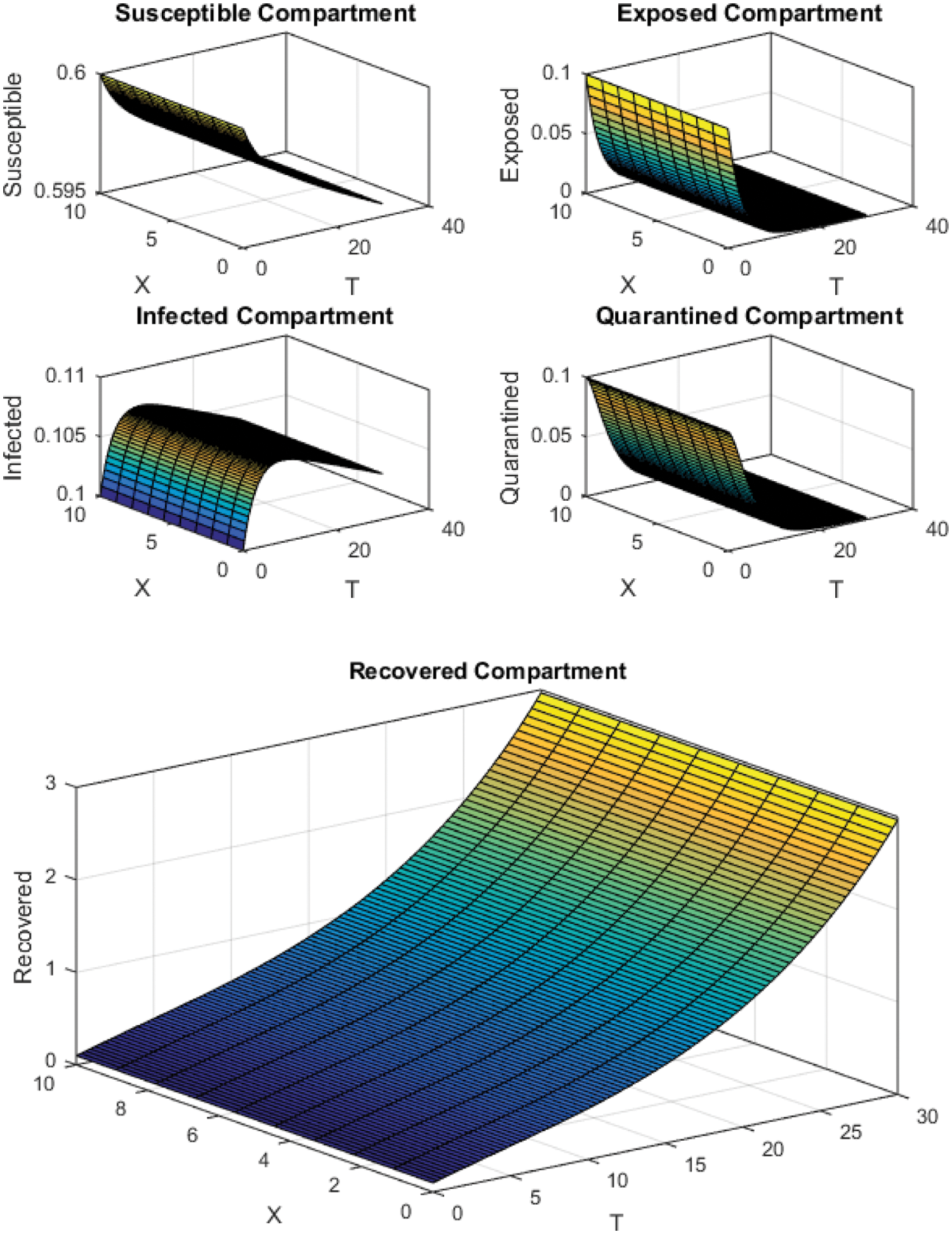
Figure 7: FTCS Scheme with
All the plots obtained through these numerical schemes show that the rate β at which susceptible individuals move to the infected and exposed class is the key element in the spreading or controlling of the pandemic. Figs. 2, 4 and 6 show that the disease becomes uncontrollable with a higher contact rate of susceptible people with infected and exposed class
The execution time for both cases of the basic reproductive number
This paper presents the COVID-19 reaction-diffusion model comprising five compartments (
Future Directions: In the present work, we have studied a reaction-diffusion COVID-19 model using first-order ordinary differential equations and discussed the non-negativity of the model. We have found the equilibrium points and discussed their stability. We have applied three numerical schemes for the simulations and discussed the characteristics of schemes like stability and consistency. Fractional calculus provides rich dynamics in fields like engineering and mathematical ecology. In the future, the present work can be studied using fractional-order derivatives.
Acknowledgement: The authors wish to express their gratitude to Prince Sultan University for facilitating the publication of this article through the Theoretical and Applied Sciences Lab.
Funding Statement: This work was supported by the research grants Seed Project; Prince Sultan University; Saudi Arabia SEED-2022-CHS-100.
Conflicts of Interest: The authors declare they have no conflicts of interest to report regarding the present study.
References
1. He, S., Peng, Y., Sun, K. (2020). SEIR modeling of the COVID-19 and its dynamics. Nonlinear Dynamics, 101(3), 1667–1680. DOI 10.1007/s11071-020-05743-y. [Google Scholar] [CrossRef]
2. Courtemanche, C., Garuccio, J., Le, A., Pinkston, J., Yelowitz, A. (2020). Strong social distancing measures in the United States reduced the COVID-19 growth rate: Study evaluates the impact of social distancing measures on the growth rate of confirmed COVID-19 cases across the United States. Health Affairs, 39(7), 1237–1246. DOI 10.1377/hlthaff.2020.00608. [Google Scholar] [CrossRef]
3. Cao, J., Tu, W. J., Cheng, W., Yu, L., Liu, Y. K. et al. (2020). Clinical features and short-term outcomes of 102 patients with coronavirus disease 2019 in Wuhan, China. Clinical Infectious Diseases, 71(15), 748–755. DOI 10.1093/cid/ciaa243. [Google Scholar] [CrossRef]
4. Ming, W. K., Huang, J., Zhang, C. J. (2020). Breaking down of healthcare system: Mathematical modelling for controlling the novel coronavirus (2019-nCoV) outbreak in Wuhan, China. DOI 10.1101/2020.01.27.922443. [Google Scholar] [CrossRef]
5. Nesteruk, I. (2020). Statistics based predictions of coronavirus 2019-nCoV spreading in mainland China. DOI 10.1101/2020.02.12.20021931. [Google Scholar] [CrossRef]
6. McKibbin, W., Fernando, R. (2021). The global macroeconomic impacts of COVID-19: Seven scenarios. Asian Economic Papers, 20(2), 1–30. DOI 10.1162/asep_a_00796. [Google Scholar] [CrossRef]
7. Ivanov, D., Dolgui, A. (2020). Viability of intertwined supply networks: Extending the supply chain resilience angles towards survivability. A position paper motivated by COVID-19 outbreak. International Journal of Production Research, 58(10), 2904–2915. DOI 10.1080/00207543.2020.1750727. [Google Scholar] [CrossRef]
8. Papo, D., Righetti, M., Fadiga, L., Biscarini, F., Zanin, M. (2020). A minimal model of hospital patients’ dynamics in COVID-19. Chaos, Solitons & Fractals, 140(3), 110157. DOI 10.1016/j.chaos.2020.110157. [Google Scholar] [CrossRef]
9. Batista, M. (2020). Estimation of the final size of the second phase of the coronavirus COVID-19 epidemic by the logistic model. DOI 10.1101/2020.03.11.20024901. [Google Scholar] [CrossRef]
10. Okhuese, V. A. (2020). Mathematical predictions for coronavirus as a global pandemic. SSRN Electronic Journal. DOI 10.1101/2020.03.19.20038794. [Google Scholar] [CrossRef]
11. Aronson, J. K., Ferner, R. E. (2020). Drugs and the renin-angiotensin system in COVID-19. BMJ, 369, m1313. DOI 10.1136/bmj.m1313. [Google Scholar] [CrossRef]
12. Henry, B. M., Vikse, J., Benoit, S., Favaloro, E. J., Lippi, G. (2020). Hyperinflammation and derangement of renin-angiotensin-aldosterone system in COVID-19: A novel hypothesis for clinically suspected hypercoagulopathy and microvascular immunothrombosis. Clinica Chimica Acta, 507(6), 167–173. DOI 10.1016/j.cca.2020.04.027. [Google Scholar] [CrossRef]
13. Govindan, K., Mina, H., Alavi, B. (2020). A decision support system for demand management in healthcare supply chains considering the epidemic outbreaks: A case study of coronavirus disease 2019 (COVID-19). Transportation Research Part E: Logistics and Transportation Review, 138(1), 101967. DOI 10.1016/j.tre.2020.101967. [Google Scholar] [CrossRef]
14. Hamidian Jahromi, A., Mazloom, S., Ballard, D. (2020). What the European and American health care systems can learn from China COVID-19 epidemic; action planning using purpose designed medical telecommunication, courier services, home-based quarantine, and COVID-19 walk-in centers. Immunopathol Persa, 6(2), e17. DOI 10.34172/ipp.2020.17. [Google Scholar] [CrossRef]
15. Mao, K., Zhang, H., Yang, Z. (2020). Can a paper-based device trace COVID-19 sources with wastewater-based epidemiology? Environmental Science & Technology, 54(7), 3733–3735. DOI 10.1021/acs.est.0c01174. [Google Scholar] [CrossRef]
16. van den Driessche, P., Watmough, J. (2008). Further notes on the basic reproduction number. Mathematical Epidemiology, 159–178. [Google Scholar]
17. Mickens, R. E. (1994). Nonstandard finite difference models of differential equations. World Scientific. DOI 10.1142/2081. [Google Scholar] [CrossRef]
18. Mickens, R. E. (2007). Calculation of denominator functions for nonstandard finite difference schemes for differential equations satisfying a positivity condition. Numerical Methods for Partial Differential Equations: An International Journal, 23(3), 672–691. DOI 10.1002/(ISSN)1098-2426. [Google Scholar] [CrossRef]
19. Zeb, A., Alzahrani, E., Erturk, V. S., Zaman, G. (2020). Mathematical model for coronavirus disease 2019 (COVID-19) containing isolation class. BioMed Research International, 2020, 1–7. DOI 10.1155/2020/3452402. [Google Scholar] [CrossRef]
20. Yadav, R. P., Verma, R. (2020). A numerical simulation of fractional order mathematical modeling of COVID-19 disease in case of Wuhan China. Chaos, Solitons & Fractals, 140, 110124. DOI 10.1016/j.chaos.2020.110124. [Google Scholar] [CrossRef]
21. Sauber-Schatz, E. CDC COVID-19 Response Team. (2020). Severe outcomes among patients with coronavirus disease 2019 (COVID-19)—United States. Morbidity and Mortality Weekly Report, 69(12). [Google Scholar]
22. Nabi, K. N., Abboubakar, H., Kumar, P. (2020). Forecasting of COVID-19 pandemic: From integer derivatives to fractional derivatives. Chaos, Solitons & Fractals, 141(1), 110283. DOI 10.1016/j.chaos.2020.110283. [Google Scholar] [CrossRef]
23. Alkahtani, B. S. T., Alzaid, S. S. (2020). A novel mathematics model of COVID-19 with fractional derivative. Stability and numerical analysis. Chaos, Solitons & Fractals, 138, 110006. [Google Scholar]
24. Ahmed, N., Korkamaz, A., Rehman, M. A., Rafiq, M., Ali, M. et al. (2021). Computational modelling and bifurcation analysis of reaction diffusion epidemic system with modified nonlinear incidence rate. International Journal of Computer Mathematics, 98(3), 517–535. DOI 10.1080/00207160.2020.1759801. [Google Scholar] [CrossRef]
25. Anzum, R., Islam, M. Z. (2021). Mathematical modeling of coronavirus reproduction rate with policy and behavioral effects. DOI 10.1101/2020.06.16.20133330. [Google Scholar] [CrossRef]
26. Yousefpour, A., Jahanshahi, H., Bekiros, S. (2020). Optimal policies for control of the novel coronavirus disease (COVID-19) outbreak. Chaos, Solitons & Fractals, 136, 109883. DOI 10.1016/j.chaos.2020.109883. [Google Scholar] [CrossRef]
27. Alqarni, M. S., Alghamdi, M., Muhammad, T., Alshomrani, A. S., Khan, M. A. (2020). Mathematical modeling for novel coronavirus (COVID-19) and control. Numerical Methods for Partial Differential Equations, 38(4), 760–776. DOI 10.1002/num.22695. [Google Scholar] [CrossRef]
28. Ozarslan, R., Bas, E., Baleanu, D., Acay, B. (2020). Fractional physical problems including wind-influenced projectile motion with Mittag-Leffler kernel. AIMS Mathematics, 5(1), 467–481. DOI 10.3934/math.2020031. [Google Scholar] [CrossRef]
29. Erdal, B. A. S. (2016). Inverse singular spectral problem via Hocshtadt-Lieberman method. Communications Faculty of Sciences University of Ankara Series A1 Mathematics and Statistics, 65(2), 89–96. [Google Scholar]
30. Ozarslan, R., Bas, E. (2020). Kinetic model for drying in frame of generalized fractional derivatives. Fractal and Fractional, 4(2), 17. DOI 10.3390/fractalfract4020017. [Google Scholar] [CrossRef]
31. Arif, M. S., Raza, A., Abodayeh, K., Rafiq, M., Nazeer, A. (2020). A numerical efficient technique for the solution of susceptible infected recovered epidemic model. Computer Modeling in Engineering & Sciences, 124(2), 477–491. DOI 10.32604/cmes.2020.011121. [Google Scholar] [CrossRef]
32. Noor, M. A., Raza, A., Arif, M. S., Rafiq, M., Nisar, K. S. et al. (2022). Non-standard computational analysis of the stochastic COVID-19 pandemic model: An application of computational biology. Alexandria Engineering Journal, 61(1), 619–630. DOI 10.1016/j.aej.2021.06.039. [Google Scholar] [CrossRef]
33. Shatanawi, W., Raza, A., Arif, M. S., Abodayeh, K., Rafiq, M. et al. (2020). Design of nonstandard computational method for stochastic susceptible-infected–treated-recovered dynamics of coronavirus model. Advances in Difference Equations, 2020(1), 1–15. DOI 10.1186/s13662-020-02960-y. [Google Scholar] [CrossRef]
34. Jódar, L., Villanueva, R. J., Arenas, A. J., González, G. C. (2008). Nonstandard numerical methods for a mathematical model for influenza disease. Mathematics and Computers in Simulation, 79(3), 622–633. DOI 10.1016/j.matcom.2008.04.008. [Google Scholar] [CrossRef]
35. Twizell, E. H., Wang, Y., Price, W. G. (1990). Chaos-free numerical solutions of reaction-diffusion equations. Proceedings of the Royal Society of London. Series A: Mathematical and Physical Sciences, 430(1880), 541–576. [Google Scholar]
36. Wei, Z., Zhu, B., Yang, J., Perc, M., Slavinec, M. (2019). Bifurcation analysis of two disc dynamos with viscous friction and multiple time delays. Applied Mathematics and Computation, 347, 265–281. DOI 10.1016/j.amc.2018.10.090. [Google Scholar] [CrossRef]
37. Abodayeh, K., Raza, A., Arif, M. S., Rafiq, M., Bibi, M. et al. (2020). Stochastic numerical analysis for impact of heavy alcohol consumption on transmission dynamics of gonorrhoea epidemic. Computers, Materials & Continua, 62(3), 1125–1142. DOI 10.32604/cmc.2020.08885. [Google Scholar] [CrossRef]
38. Raza, A., Rafiq, M., Baleanu, D., Arif, M. S. (2020). Numerical simulations for stochastic meme epidemic model. Advances in Difference Equations, 2020(1), 1–16. DOI 10.1186/s13662-020-02593-1. [Google Scholar] [CrossRef]
39. Farman, M., Akgül, A., Ahmad, A., Baleanu, D., Saleem, M. U. (2021). Dynamical transmission of coronavirus model with analysis and simulation. Computer Modeling in Engineering and Sciences, 127(2), 753–769. DOI 10.32604/cmes.2021.014882. [Google Scholar] [CrossRef]
40. Savasan, A., Bilgen, K., Gokbulut, N., Hincal, E., Yoldascan, E. (2022). Sensitivity analysis of COVID-19 in mediterranean Island. Computer Modeling in Engineering & Sciences, 130(1), 133–148. DOI 10.32604/cmes.2022.017815. [Google Scholar] [CrossRef]
Cite This Article
 Copyright © 2023 The Author(s). Published by Tech Science Press.
This work is licensed under a Creative Commons Attribution 4.0 International License , which permits unrestricted use, distribution, and reproduction in any medium, provided the original work is properly cited.
 Downloads
 Citation Tools