A Weighted Average Finite Difference Scheme for the Numerical Solution of Stochastic Parabolic Partial Differential Equations

Dumitru Baleanu; Mehran Namjoo; Ali Mohebbian; Amin Jajarmi

doi:10.32604/cmes.2022.022403

icon Open Access

ARTICLE

A Weighted Average Finite Difference Scheme for the Numerical Solution of Stochastic Parabolic Partial Differential Equations

Dumitru Baleanu^1,2,3, Mehran Namjoo⁴, Ali Mohebbian⁴, Amin Jajarmi^5,*

1 Department of Mathematics, Faculty of Arts and Sciences, Çankaya University, Ankara, 06530, Turkey
2 Institute of Space Sciences, Magurele-Bucharest, R 76900, Romania
3 Department of Medical Research, China Medical University Hospital, China Medical University, Taichung, 40402, Taiwan
4 Department of Mathematics, Vali-e-Asr University of Rafsanjan, Rafsanjan, 77188-97111, Iran
5 Department of Electrical Engineering, University of Bojnord, Bojnord, 94531-1339, Iran

* Corresponding Author: Amin Jajarmi. Email: email

Computer Modeling in Engineering & Sciences 2023, 135(2), 1147-1163. https://doi.org/10.32604/cmes.2022.022403

Received 08 March 2022; Accepted 07 June 2022; Issue published 27 October 2022

Abstract

In the present paper, the numerical solution of Itô type stochastic parabolic equation with a time white noise process is imparted based on a stochastic finite difference scheme. At the beginning, an implicit stochastic finite difference scheme is presented for this equation. Some mathematical analyses of the scheme are then discussed. Lastly, to ascertain the efficacy and accuracy of the suggested technique, the numerical results are discussed and compared with the exact solution.

Keywords

Itô equation; stochastic process; finite difference scheme; stability and convergence; consistency

1 Introduction

Stochastic partial differential equations (SPDEs) driven by white noise are one of the essential classes of partial differential equations (PDEs). This class of equations arises in many branches of applied sciences and engineering, such as nonlinear filtering [1], turbulent flows [2], population biology [3], microscopic particle dynamics [4], groundwater flow [5], etc. Few numbers of SPDEs can be solved by analytical techniques [6], most of which cannot be analyzed by well-known analytical schemes suitably. Due to this reason, various numerical methods have been discussed to solve such equations [7–9]. For instance, the authors in [10] proposed an explicit scheme to obtain the approximate solution of stochastic equations. In [11], a compact finite difference method for solving a stochastic advection-diffusion equation was proposed. In [12], two techniques on the basis of Saul’yev method and finite difference scheme were suggested for solving linear SPDEs. In [13], explicit and implicit finite difference methods were proposed to obtain the solution of general SPDEs. In [14], a stochastic compact finite difference scheme was suggested for solving a stochastic fractional advection-diffusion equation. In [15], high-resolution finite volume methods were used to solve SPDEs. In [16], the authors proposed a spectral collocation method for the numerical solution of SPDEs driven by infinite dimensional fractional Brownian motions. More than these, some authors used spectral methods for the discretization of spatial variables and applied a Crank-Nicolson scheme or a stochastic Runge-Kutta method for solving the resultant system of stochastic differential equations [17].

In [18,19], the authors investigated the convergence and stability of two stochastic finite difference schemes for a class of SPDEs. In more detail, the study [19] employed a Crank-Nicolson technique for the approximation of second-order derivatives. Although the reported results in [18,19] are interesting in some senses, the solution methods presented are only conditionally stable. To overcome this issue, here we extend a type of finite difference scheme to a stochastic version in order to approximate the solution of a stochastic advection-diffusion equation. To do so, instead of the Crank-Nicolson method used in [19], we consider a convex combination of discretized second-order derivatives in two consecutive time grid points. As a result, the proposed method in our case is unconditionally stable under a necessary condition, so there will be no limitation for the selection of space and time step sizes. This important feature makes the computational cost of our suggested technique less than the other methods available in the literature [18,19]. In the following, the main contributions of our study are summarized and highlighted as below:

• In this paper, a stochastic finite difference scheme is developed for the numerical solution of Itô type stochastic parabolic equation.

• As a theoretical investigation, some mathematical results for the proposed scheme are studied.

• In addition, the convergence of the suggested technique is discussed, and the necessary conditions for its conditional and unconditional stability are explored.

• Finally, the efficiency of the proposed method is shown by some numerical examples, and its key qualifications are examined as well.

The rest of this paper is structured as follows. An implicit finite difference scheme is proposed in Section 2, where some mathematical analyses are also investigated. Next, some numerical results are given in Section 3. Finally, the paper is closed by some concluding remarks in the last section.

2 Proposed Scheme

In this work, the following problem for the stochastic equation of Itô type is considered:

$∂v∂t=ρ∂2v∂x2(x,t)+σv(x,t)ξ˙(t),v(x,0)=v0(x),v(0,t)=f1(t),v(1,t)=f2(t),$ (1)

for $x∈(0,1)$ and $t∈(0,1]$ . In this problem, the coefficients $ρ$ and $σ$ are constants, and $ξ(t)$ indicates a standard Wiener process. Also, the noise term $ξ˙(t)$ is introduced to present a time white noise. Formally, $ξ˙(t)$ is a Gaussian distribution with zero mean value [20].

Finite difference schemes are the most natural way of solving PDEs numerically. Furthermore, these methods are widely used in approximating the solution of SPDEs like (1). The idea behind these schemes is to discretize the continuous time and space into a finite number of discrete grid points. Then the values of state variables are calculated at any point of the grid. By considering a uniform space grid $Δx$ and time grid $Δt$ in the time-space lattice, the solution of the equation can be estimated at the lattice points. The value of the approximate solution at the point $(hΔx,mΔt)$ is indicated by the random variable $vhm$ , where m and h are integer. The later stage is to approximate the problem (1) on the mentioned grid. For this purpose, the time and the space derivatives in the SPDE (1) are replaced by the following finite difference approximations:

$vt(hΔx,mΔt)≈vhm+1−vhmΔt,vxx(hΔx,mΔt)≈λvh−1m+1−2vhm+1+vh+1m+1Δx2+(1−λ)vh−1m−2vhm+vh+1mΔx2,$ (2)

where $0≤λ≤1$ . Indeed, we use a forward finite difference scheme for the approximation of $vt(hΔx,mΔt)$ as

$vt(hΔx,mΔt)=v(hΔx,(m+1)Δt)−v(hΔx,mΔt)Δt+O(Δt),$ (3)

and employ a convex combination of second-order derivatives in the time steps m and $m+1$ for the approximation of $vxx(hΔx,mΔt)$ by

$vxx(hΔx,mΔt)=λv((h−1)Δx,(m+1)Δt)−2v(hΔx,mΔt)+v((h+1)Δx,(m+1)Δt)Δx2+(1−λ)v((h−1)Δx,mΔt)−2v(hΔx,mΔt)+v((h+1)Δx,mΔt)Δx2+O(Δx2).$ (4)

For more details, the interested reader can refer to [21]. Substituting the approximations from (2) into (1), we can find

$−λrvh−1m+1+(1+2λr)vhm+1−λrvh+1m+1=(1−λ)rvh−1m+(1−2(1−λ)r)vhm+(1−λ)rvh+1m+σvhmΔξm,$ (5)

where $r=ρΔtΔx2$ , and $Δξm=ξ((m+1)Δt)−ξ(mΔt)$ is a Gaussian distribution with zero mean value and variance $Δt$ , i.e., $Δξm∼N(0,Δt).$

Remark 2.1. In the proposed scheme, the Wiener process increments are not dependent on the state $vhm$ .

Substantially, the convergence of the stochastic difference scheme to the SPDE solution is very important. To achieve this, consider an SPDE in the form of $Lu=F,$ wherein F is an inhomogeneity and L represents the differential operator. Suppose that the random variable $vhm$ be a solution that is approximated by a stochastic finite difference scheme indicated by $Lhm$ . By applying the stochastic scheme to this SPDE, we obtain

$Lhmvhm=Fhm,$ (6)

where $Fhn$ is the approximation of inhomogeneity $F$ . In favor of accessing the consistency, stability, and convergence results, a norm is needed. Because of this, for the sequence $v={…,v−1,v0,v1,…}$ , we define the $sup$ –norm as $‖v‖∞=suph|vh|2$ . For additional details concerning the concepts of consistency, stability and convergence, see [10].

Definition 2.1. A stochastic finite difference scheme $Lhmvhm=Fhm$ is said to be point-wise consistent in mean square with PDE $Lu=F$ at point $(x,t)$ , if for any continuously differentiable solution $Υ=Υ(x,t)$ of this equation, we have

$E‖(LΥ−F)|hm−[LhmΥ(hΔx,mΔt)−Fhm]‖2→0,$

as $(Δx,Δt)→(0,0)$ and $(hΔx,(m+1)Δt)→(x,t).$

Theorem 2.1. The numerical scheme (5) is consistent in mean square in the sense of Definition 2.1.

Proof. For the smooth function $Υ(x,t)$ , we have

$L(Υ)|hm=Υ(hΔx,(m+1)Δt)−Υ(hΔx,mΔt)−ρ∫mΔt(m+1)ΔtΥxx(hΔx,w)dw−σ∫mΔt(m+1)ΔtΥ(hΔx,w)dξ(w),$ (7)

and

$LhmΥ=Υ(hΔx,(m+1)Δt)−Υ(hΔx,mΔt)−σΥ(hΔx,mΔt)(ξ((m+1)Δt)−ξ(mΔt))−ρλΔtΥ((h−1)Δx,(m+1)Δt)−2Υ(hΔx,(m+1)Δt)+Υ((h+1)Δx,(m+1)Δt)Δx2−ρ(1−λ)ΔtΥ((h−1)Δx,mΔt)−2Υ(hΔx,mΔt)+Υ((h+1)Δx,mΔt)Δx2.$ (8)

Accordingly,

$E|L(Υ)|hm−LhmΥ|2≤2ρ2E|∫mΔt(m+1)Δt[Υxx(hΔx,w)−1Δx2(λ[Υ((h−1)Δx,(m+1)Δt)−2Υ(hΔx,(m+1)Δt)+Υ((h+1)Δx,(m+1)Δt)]+(1−λ)[Υ((h−1)Δx,mΔt)−2Υ(hΔx,mΔt)+Υ((h+1)Δx,mΔt)])]dw|2+2σ2∫mΔt(m+1)Δt|Υ(hΔx,w)−Υ(hΔx,mΔt)|2dw.$ (9)

In as much as $Υ(x,t)$ is a deterministic function, $E|L(Υ)|hm−LhmΥ|2→0$ as $m,h→∞$ . Hence, the numerical scheme (5) is consistent with the SPDE (1).

By the assumption that $v^m+1$ is the Fourier transform of $vm+1$ , the Fourier inversion formula results in

$vnm+1=12π∫−πΔxπΔxeinΔxηv^m+1(η)dη,$ (10)

where

$v^m+1=12π∑n=−∞∞e−inΔxηvnm+1Δx,$ (11)

and $η$ is a real variable. We utilize the Von Neumann method to investigate the stability of the stochastic difference scheme. By substituting Eq. (11) into the stochastic difference equation and using the equality of Fourier transformation, one achieves

$v^m+1(η)=v^m(η)g(Δxη,Δt,Δx),$ (12)

where $v^m$ is the Fourier transform of $vm$ . Therefore,

$E|g(Δxη,Δt,Δx)|2≤1+KΔt,$ (13)

will be the necessary and sufficient condition for the stability [10].

Theorem 2.2. For the stochastic advection-diffusion Eq. (1), the stochastic scheme (5) is unconditionally stable for $λ≥12$ based on the Fourier transformation analysis, and is conditionally stable for $λ≤12$ under the condition $r≤12(1−2λ)$ .

Proof. Substituting (11) into (5), we get

$(−λre−iΔxη+(1+2λr)−λreiΔxη)v^m+1(η)=((1−λ)re−iΔxη+(1−2(1−λ)r)+(1−λ)reiΔxη+σΔξm)v^m(η).$ (14)

Then we have

$v^m+1(η)=(1−λ)re−iΔxη+(1−2(1−λ)r)+(1−λ)reiΔxη−λre−iΔxη+(1+2λr)−λreiΔxη+σΔξm(1−λ)re−iΔxη+(1−2(1−λ)r)+(1−λ)reiΔxηv^m(η).$ (15)

Hence, the stochastic difference scheme amplification factor is

$g(Δxη,Δt,Δx)=(1−λ)re−iΔxη+(1−2(1−λ)r)+(1−λ)reiΔxη−λre−iΔxη+(1+2λr)−λreiΔxη+σΔξm(1−λ)re−iΔxη+(1−2(1−λ)r)+(1−λ)reiΔxη=1−4(1−λ)rsin2⁡Δxη21+4λrsin2⁡Δxη2+σ21+4λrsin2⁡Δxη2Δt.$ (16)

Set $χ(Δxη)=1−4(1−λ)rsin2⁡Δxη21+4λrsin2⁡Δxη2$ , so $χ(θ)=1−4(1−λ)rsin2⁡θ21+4λrsin2⁡θ2$ . Now, by setting the derivative of $χ(θ)$ equal to zero, the critical points are obtained as $θ=0,±π$ . Then one notes that $χ(0)=1$ and

$χ(±π)=1−4(1−λ)r1+4λr.$ (17)

It is easy to see that $1−4(1−λ)r1+4λr≤1$ . Since the equation

$−1≤1−4(1−λ)r1+4λr,$ (18)

is equivalent to $4r(1−2λ)≤2$ , clearly if $λ≥12$ , then the inequality (18) is always satisfied, and if $λ<12$ , then the inequality (18) is satisfied only if

$r≤12(1−2λ).$ (19)

And also

$|11+4λrsin2⁡Δxη2|≤1,$

is always satisfied. Hence, we see that if $λ≥12$ , the scheme (5) is unconditionally stable, and if $λ<12$ , the difference scheme (5) is conditionally stable with the condition for the stability given by (19).

Definition 2.2. The stochastic difference scheme $Lhmvhm=Fhm$ , which approximates the SPDE $Lu=F$ , is convergent in mean square at time t when $(m+1)Δt$ converges to $t$ , $E‖vm+1−um+1‖2→0$ for $(m+1)Δt=t$ , $Δx→0$ , and $Δt→0$ .

Theorem 2.3. The numerical scheme (5) for the Eq. (1) is convergent in mean square with respect to $‖⋅‖∞=suph|⋅|2$ with $r≤12(1−λ)$ and $t=(m+1)Δt$ .

Proof. The stochastic finite difference scheme is given by

$vhm+1=vhm+ρΔt((1−λ)vh+1m−2vhm+vh−1mΔx2+λvh+1m+1−2vhm+1+vh−1m+1Δx2)+σvhm(ξ((m+1)Δt)−ξ(mΔt)).$ (20)

The solution $uhm+1$ is represented by the Taylor’s expansion $uxx(x,w)$ with respect to the space variable as follows:

$uhm+1=uhm+ρ∫mΔt(m+1)Δtuxx(xh,w)dw+σ∫mΔt(m+1)Δtu(xh,w)dξ(w)=uhm+ρ∫mΔt(m+1)Δt((1−λ)uh+1m−2uhm+uh−1mΔx2+λuh+1m+1−2uhm+1+uh−1m+1Δx2−Δx24!((1−λ)[uxxxx((h+β1)Δx,w)+uxxxx((h+β2)Δx,w)]+λ[uxxxx((h+β3)Δx,w+Δt)+uxxxx((h+β4)Δx,w+Δt)])−λΔtuxxt(hΔx,w+δΔt))dw+σ∫mΔt(m+1)Δtu(xh,w)dξ(w),$ (21)

where $β1,β2,β3,β4,Δ∈(0,1)$ . Then we have

$uhm+1=uhm+ρ∫mΔtΔt+mΔt(λuh+1m+1−2uhm+1+uh−1m+1Δx2+(1−λ)uh+1m−2uhm+uh−1mΔx2−Δx24!((1−λ)[uxxxx((h+β1)Δx,w)+uxxxx((h+β2)Δx,w)]+λ[uxxxx((h+β3)Δx,w+Δt)+uxxxx((h+β4)Δx,w+Δt)])−λρΔtuxxxx(hΔx,w+δΔt))dw−Δtλσ∫mΔtΔt+mΔtuxx(xh,w)dξ(w)+σ∫mΔtΔt+mΔtu(xh,w)dξ(w).$ (22)

Let $zhm=uhm−vhm$ , so we get

$zhm+1=zhm+ρ∫mΔtΔt+mΔt((1−λ)zh+1m−2zhm+zh−1mΔx2+λzh+1m+1−2zhm+1+zh−1m+1Δx2−Δx24!((1−λ)[uxxxx((h+β1)Δx,w)+uxxxx((h+β2)Δx,w)]+λ[uxxxx((h+β3)Δx,w+Δt)+uxxxx((h+β4)Δx,w+Δt)])−λρΔtuxxxx(hΔx,w+δΔt))dw−λσΔt∫mΔtΔt+mΔtuxx(x,w)|x=xhdξ(w)+σ∫mΔtΔt+mΔt(u(x,w)|x=xh−vhm)dξ(w).$ (23)

It gives that

$−λrzh−1m+1+(1+2λr)zhm+1−λrzh+1m+1=(1−λ)rzh−1m+(1−2(1−λ)r)zhm+(1−λ)rzh+1m+ρ∫mΔtΔt+mΔt[−Δx24!((1−λ)[uxxxx((h+β1)Δx,w)+uxxxx((h+β2)Δx,w)]+λ[uxxxx((h+β3)Δx,w+Δt)+uxxxx((h+β4)Δx,w+Δt)])−λρΔtuxxxx(hΔx,w+δΔt)]dw−λσΔt∫mΔtΔt+mΔtuxx(x,w)|x=xhdξ(w)+σ∫mΔtΔt+mΔt(u(x,w)|x=xh−vhm)dξ(w),$ (24)

where $r=ρΔtΔx2$ . Applying $E|⋅|2$ to the above equation and using the following inequality:

$E|X+Y+Z+R|2≤8E|Z|2+8E|Y|2+2E|R|2+4E|X|2,$

we have

$E|λrzh−1m+1+(1+2λr)zhm+1−λrzh+1m+1|2≤4E|(1−λ)rzh−1m+(1−2(1−λ)r)zhm+(1−λ)rzh+1m|2+8E|ρ∫mΔtΔt+mΔt[−Δx24!((1−λ)[uxxxx((h+β1)Δx,w)+uxxxx((h+β2)Δx,w)]+λ[uxxxx((h+β3)Δx,w+Δt)+uxxxx((h+β4)Δx,w+Δt)])−λρΔtuxxxx(hΔx,w+δΔt)]dw|2+8(λσΔt)2E|∫mΔtΔt+mΔtuxx(x,w)|x=xhdξ(w)|2+4σ2∫mΔtΔt+mΔtE|u(x,w)|x=xh−uhm|2dw+4σ2∫mΔt(m+1)ΔtE|uhm−vhm|2dw⏟E|zhm|2Δt,$ (25)

and so

By introducing the notation $Θ1h=uxxxx((h+β1)Δx,s)<∞$ , $Θ2h=uxxxx((h+β2)Δx,s)<∞$ , $Θ3h=uxxxx((h+β3)Δx,s+Δt)<∞$ , $Θ4h=uxxxx((h+β4)Δx,s+Δt)<∞$ , $Θ5h=uxxxx(hΔx,s+δΔt)<∞$ , $ψ1h=uxx(x,s)<∞$ , taking into account

and the usage of supposition $r≤12(1−λ)$ , one concludes that

Therefore,

$(−|λr|+|1+2λr|−|λr|)2suphE|zhm+1|2≤8suphE|ψ1|2Δt+8suphE|ψ2|2Δt+ψ4Δt+4suphE|zhm|2(1+σ2Δt),$ (29)

and

$suphE|zhm+1|2≤ψΔt+4suphE|zhm|2(1+σ2Δt).$ (30)

It gives that

$E‖zm+1‖∞2≤ψΔt+(4+4σ2Δt)E‖zm‖∞2≤ψΔt+(σ2tm+1+1)m+1∑k=1m(4ψΔt)k≤eσ2t∑k=1m(4ψΔt)k+ψΔt.$ (31)

When $Δt→0$ , we have

$E‖zm+1‖∞2≤4eσ2tψΔt+ψΔt+(m−1)eσ2t(4ψΔt)2≤teσ2tΔt(4ψ)2+(4eσ2t+1)ψΔt≤(16teσ2tψ+4eσ2t+1)ψΔt,$ (32)

and so $E‖zm+1‖∞2→0$ .

Here, it is worth mentioning that according to the inequality (32), the error of the proposed scheme (5) is of first order with respect to the time.

3 Numerical Results and Discussion

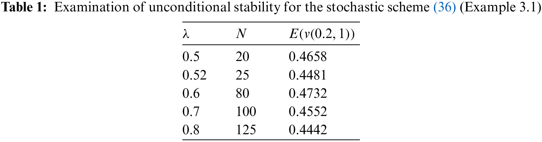
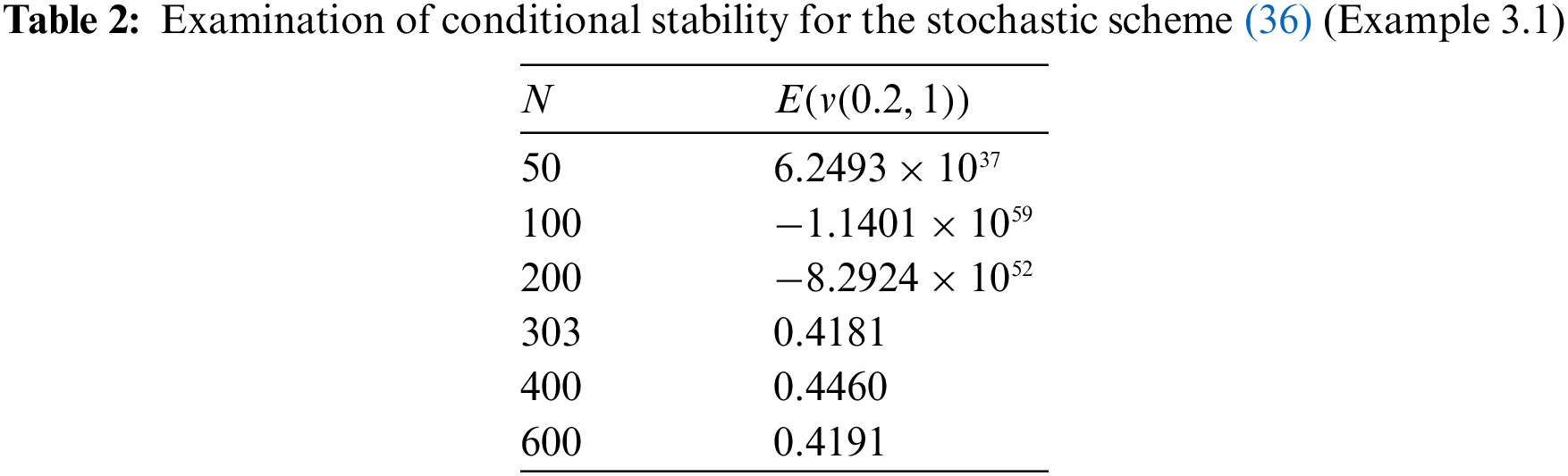
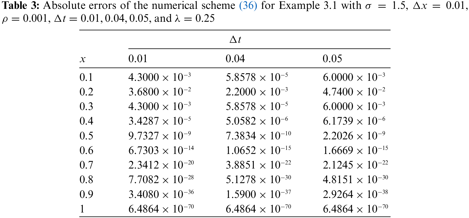
In this part, we demonstrate the efficacy and accuracy of the suggested technique, developed in the previous section, by solving some numerical examples. Indeed, we investigate the theoretical consequences of previous section about the stability and convergence of the proposed scheme (5). In more detail, we discuss the convergence of the scheme (5) for each example and explore the necessary conditions for its conditional and unconditional stability. Numerical results in this section verify the previously presented theoretical analysis.

Example 3.1. Consider an SPDE in the following form:

$vt(x,t)=ρvxx(x,t)+σv(x,t)ξ˙(t),(x,t)∈(0,1)×(0,1],$ (33)

supplemented with the initial and boundary conditions

$v(x,0)=exp⁡(−(x−0.2)2ρ),x∈(0,1),v(0,t)=14t+1exp⁡(−0.04ρ(4t+1)),t∈(0,1],v(1,t)=14t+1exp⁡(−0.64ρ(4t+1)),t∈(0,1].$ (34)

The exact solution is

$v(x,t)=exp⁡(−(x−0.2)2ρ(1+4t))1+4t,$ (35)

if there is no noise term. Following the proposed idea developed in this paper, the stochastic finite difference scheme can be written as follows:

$−λrvh−1m+1+(1+2λr)vhm+1−λrvh+1m+1=(1−λ)rvh−1m+(1−2(1−λ)r)vhm+(1−λ)rvh+1m+σvhmΔξn,$ (36)

where $r=ρΔtΔx2$ . To qualify the numerical results obtained in this example, the exact and numerical solutions are plotted in Fig. 1. Let M and N be the total numbers of grid points for the space and time discretization, respectively. If we set $ρ=0.01$ , $σ=1$ , and $M=125$ ( $Δx=0.008$ ), then according to Theorem 2.2, the stochastic finite difference scheme (36) is unconditionally stable for all $λ≥12$ (see Table 1), and it is conditionally stable for $λ<12$ with $12(1−2λ)≥r$ where $r=ρΔtΔx2$ . To test the conditional stability as well, let $λ=0.01$ ; then Theorem 2.2 implies that the numerical scheme (36) is stable for $N≥303$ , a fact which is verified by the reported results in Table 2. Also, the absolute errors of the numerical scheme (36) with $σ=1.5$ , $Δx=0.01$ , $ρ=0.001$ , $λ=0.25$ , and $Δt=0.01,0.04,0.05$ are reported in Table 3.

images

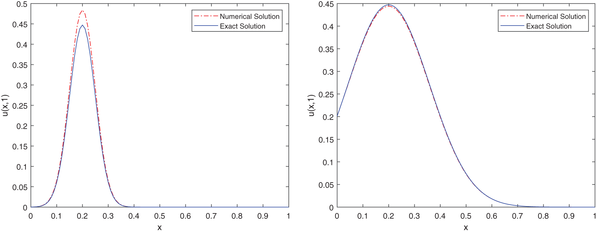
Figure 1: Comparison between the exact solution and the stochastic numerical solution of (33) with $ρ=0.01$ , $Δx=0.008$ , σ = 1, $Δt=0.008$ , $λ=0.75$ (right figure), and σ = 1.5, $Δx=0.01$ , $ρ=0.001$ , $Δt=0.01$ , $λ=0:25$ (left figure) (Example 3.1)

images

Example 3.2. Let us consider the following problem for the next example:

$vt(x,t)=v(x,t)ξ˙(t)+vxx(x,t),(x,t)∈(0,1)×(0,1],v(x,0)=sin⁡(πx),x∈(0,1),v(0,t)=v(1,t)=0,t∈(0,1],$ (37)

with the exact solution

$v(x,t)=sin⁡(πx)e−π2t.$ (38)

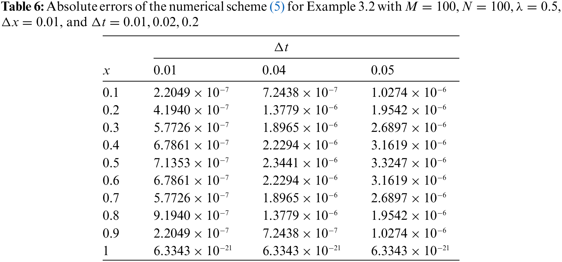
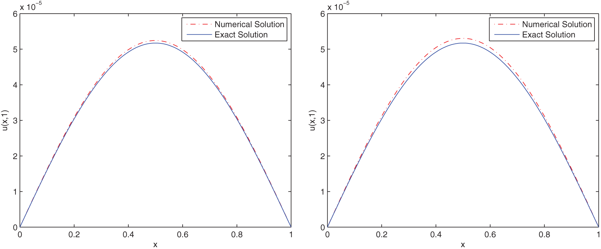
In Fig. 2, the exact solution and the stochastic numerical solution of (37) are compared for the two sets of $M=100,N=100,λ=0.5$ (left plot) and $M=120,N=120,λ=0.55$ (right plot). More comparisons between the exact and the numerical solutions are given in Fig. 3 for the values of $ρ=1,σ=1,λ=0.55,Δx=1120,Δt=0.01$ (left plot) and $ρ=1,σ=1,λ=0.5,Δx=0.01,Δt=0.02$ (right plot). From the numerical results in Figs. 2 and 3, one can see the high accuracy of the presented method for solving the SPDE (37). In Table 4, the unconditional stability of the proposed scheme (5) is shown for $λ≥12$ . For $λ=0.4$ and $M=100$ , Table 5 portrays the conditional stability of the suggested technique (5) when $N≥4000$ , a fact which is also shown in Fig. 4. In addition, the absolute errors of the numerical scheme (5) with $M=100$ , $N=100$ , $λ=0.5$ , $Δx=0.01$ , and $Δt=0.01,0.02,0.2$ are reported in Table 6.

images

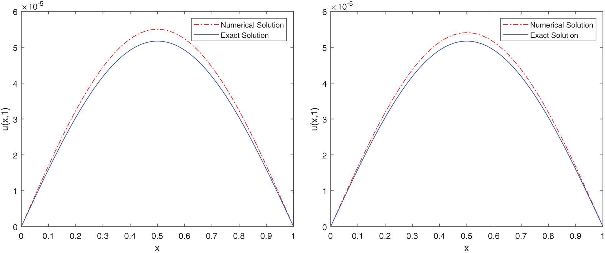
Figure 2: Comparison between the exact solution and the stochastic numerical solution of (37) with M = 100, N = 100, $λ=0.5$ (left figure), and M = 120, N = 120, $λ=0.55$ (right figure) (Example 3.2)

images

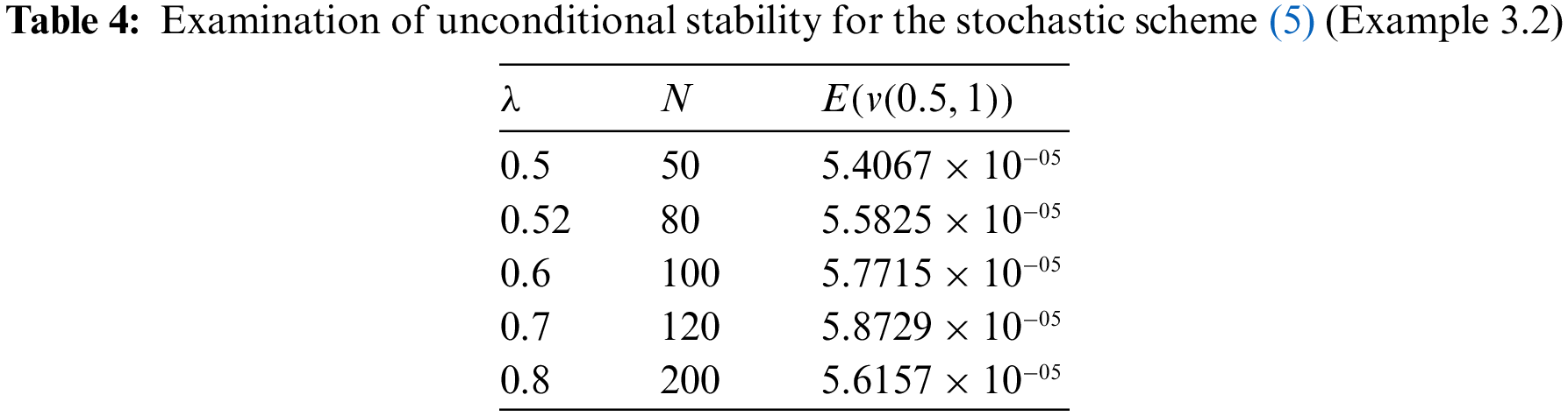
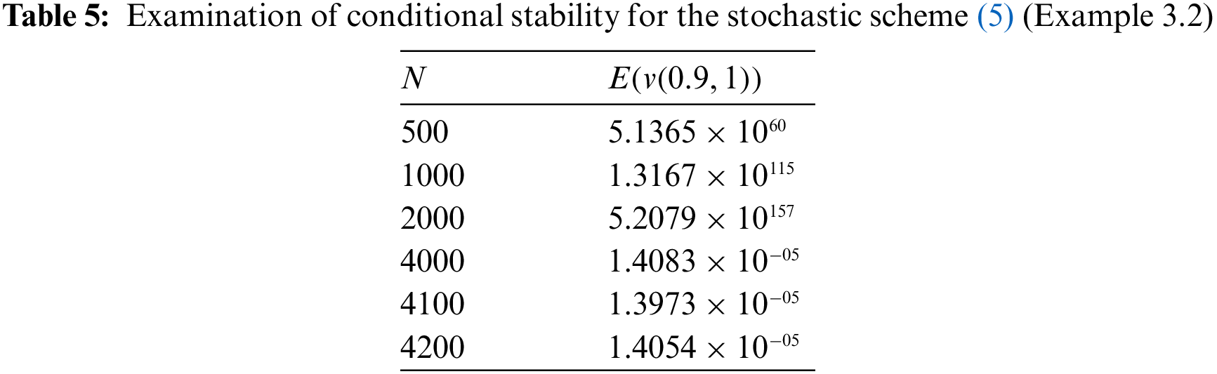
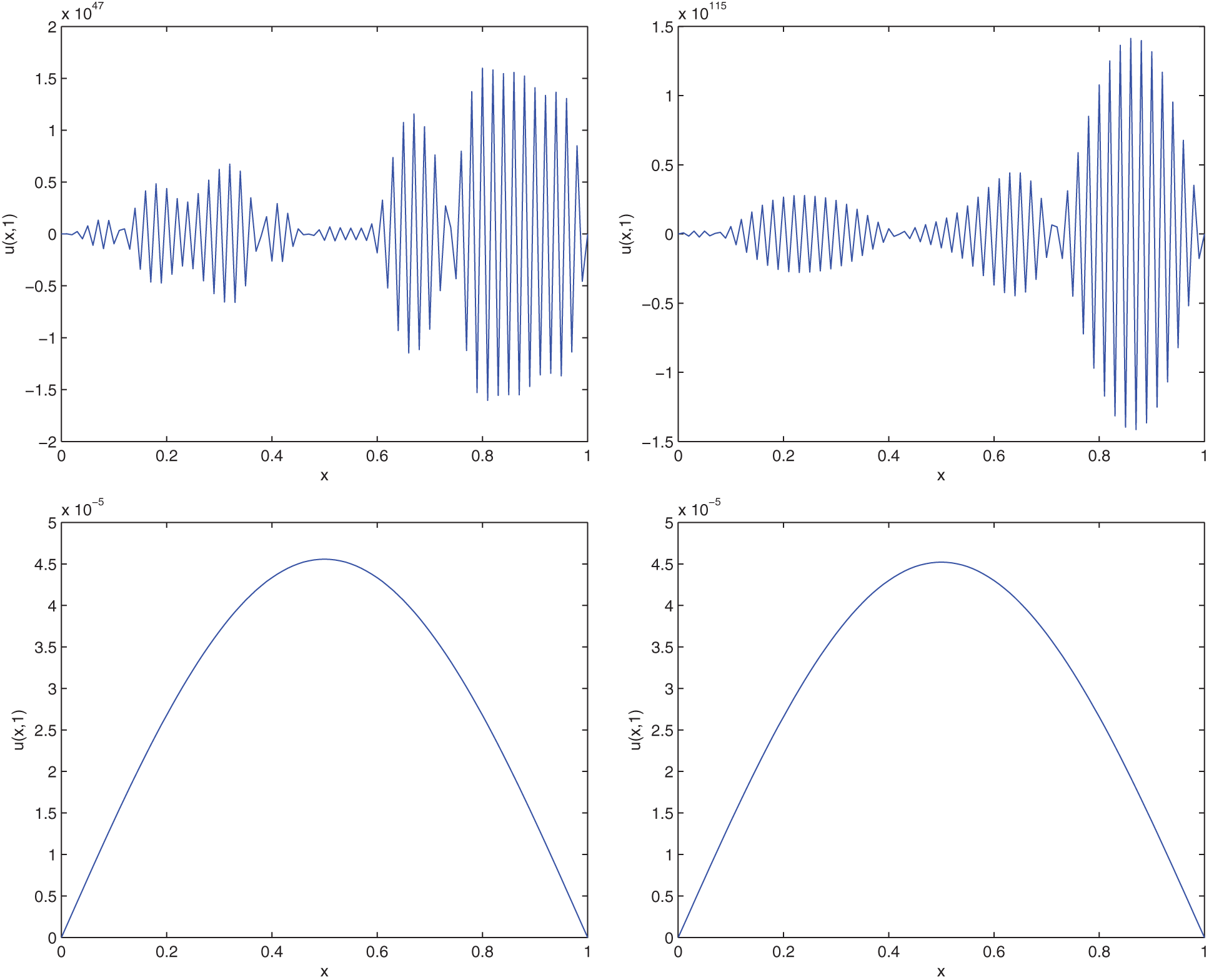
Figure 3: Comparison between the exact solution and the stochastic numerical solution of (37) with $ρ=1$ , $σ=1$ , $λ=0.55$ , $Δx=1120$ , $Δt=0.01$ (left plot), and $ρ=1$ , $σ=1$ , $λ=0.5$ , $Δx=0.01$ , $Δt=0.02$ (rightplot) (Example 3.2)

images

Figure 4: Display of conditional stability for various values of N = 400, 1000, 4000, 4100 (Example 3.2)

images

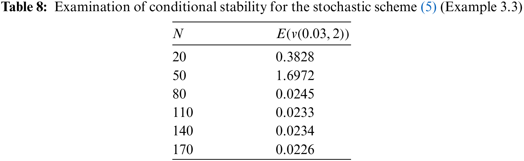
Example 3.3. As the third example, consider the following problem:

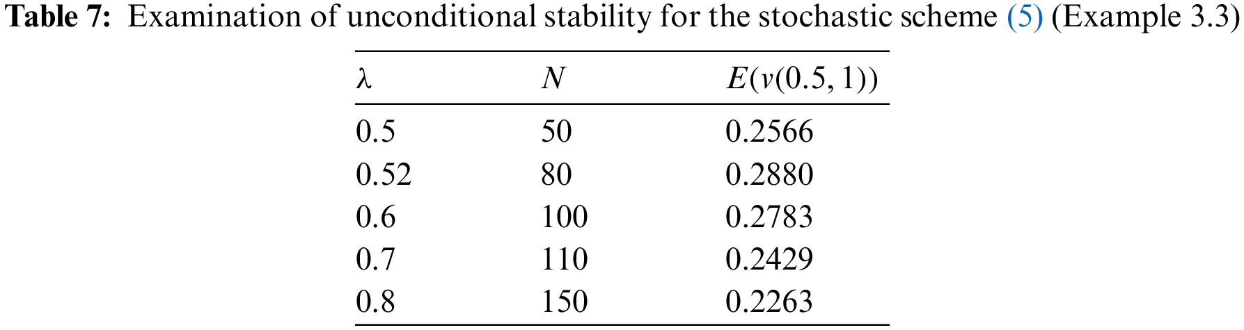
$vt(x,t)=0.01vxx(x,t)+v(x,t)ξ˙(t),(x,t)∈(0,1)×(0,1],v(x,0)=x−x2,x∈(0,1),v(0,t)=v(1,t)=0,t∈(0,1].$ (39)

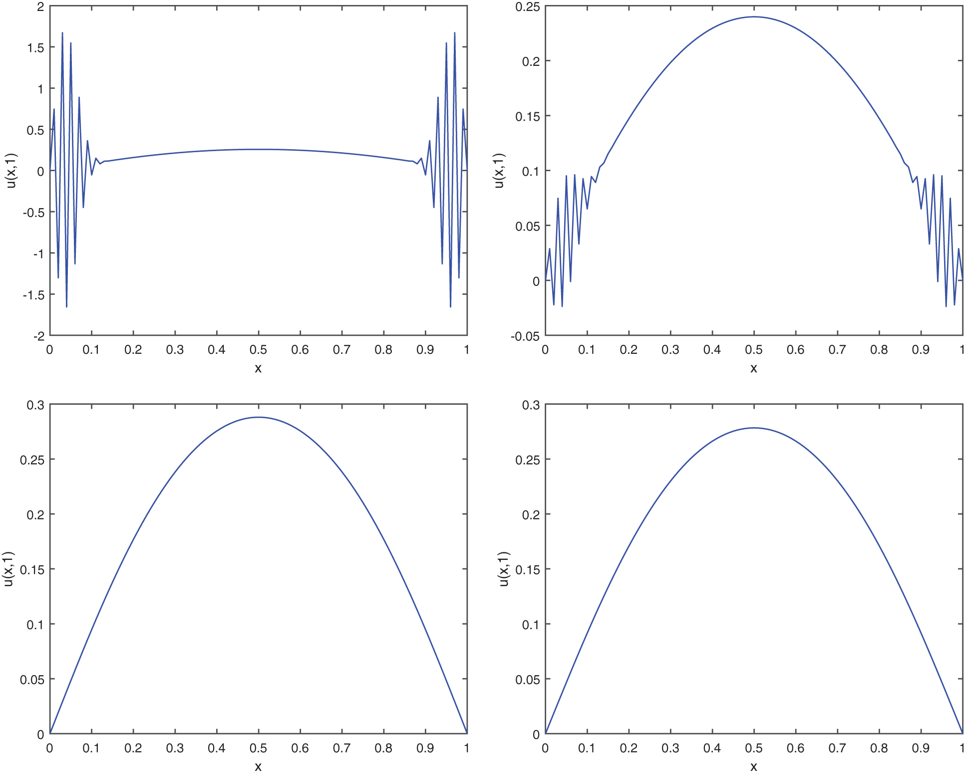
Fig. 5 shows the approximation of SPDE (39) using the stochastic difference scheme (5) with the values $N=50,60,80,100$ . In Table 7, the unconditional stability of the proposed method is depicted for $λ≥12$ . To test the conditional stability for $ρ=0.01$ , $M=100$ , and $λ=0.3$ , simulation results of (39) for various values of N are presented in Fig. 5 and Table 8. According to these results for Example 3.3, it is apparent that the stochastic finite difference scheme (5) is stable when $N≥80$ , a fact which coincides with the stability condition provided by Theorem 2.2.

images

Figure 5: Display of conditional stability for various values of N = 50, 60, 80, 100 (Example 3.3)

images

4 Conclusion

This study presented a numerical method based on the weighted average finite difference scheme for the solution of SPDEs. In this paper, we provided some mathematical analyses for the proposed numerical scheme. To ascertain the accuracy and efficacy of the proffered technique, we presented three numerical examples with different boundary conditions, and compared the associated numerical results with the exact solution. Additionally, we explored the necessary conditions for the conditional and unconditional stability of the presented method and verified the theoretical consequences in this regard by some figures and tables.

Future works can be focused on applying some new discrete schemes, such as those discussed in [22] with a second-order time convergence rate, for the numerical solution of stochastic problem studied in this paper.

Acknowledgement: The authors would like to express their deep gratitude to Dr. Fahimeh Akhavan Ghassabzade for her valuable assistance during the development of this research work.

Funding Statement: The authors received no specific funding for this study.

Conflicts of Interest: The authors declare that they have no conflicts of interest to report regarding the present study.

References

1. Zakai, M. (1969). On the optimal filtering of diffusion processes. Zeitschrift für Wahrscheinlichkeitstheorie und Verwandte Gebiete, 11, 230–243. DOI 10.1007/BF00536382. [Google Scholar] [CrossRef]

2. Mikulevicius, R., Rozovskii, B. L. (2004). Stochastic navier-stokes equations for turbulent flows. SIAM Journal on Mathematical Analysis, 35, 1250–1310. DOI 10.1137/S0036141002409167. [Google Scholar] [CrossRef]

3. Dawson, D. A., Perkins, E. A. (1999). Measure-valued processes and renormalization of branching particle systems. In: Carmona, R. A., Rozovskii, B. (Eds.Stochastic partial differential equations: Six perspectives, pp. 45–106. Providence, RI: American Mathematical Society. [Google Scholar]

4. Roques, L., Allard, D., Soubeyrand, S. (2022). Spatial statistics and stochastic partial differential equations: A mechanistic viewpoint. Spatial Statistics, 50, 100591. DOI 10.1016/j.spasta.2022.100591. [Google Scholar] [CrossRef]

5. Wang, J., Pang, X., Yin, F., Yao, J. (2022). A deep neural network method for solving partial differential equations with complex boundary in groundwater seepage. Journal of Petroleum Science and Engineering, 209, 109880. DOI 10.1016/j.petrol.2021.109880. [Google Scholar] [CrossRef]

6. Prato, G. D., Tubaro, L. (1992). Stochastic partial differential equations and application. Boca Raton: CRC Press. [Google Scholar]

7. Yasin, M. W., Iqbal, M. S., Ahmed, N., Akgül, A., Raza, A. et al. (2022). Numerical scheme and stability analysis of stochastic fitzhugh-nagumo model. Results in Physics, 32, 105023. DOI 10.1016/j.rinp.2021.105023. [Google Scholar] [CrossRef]

8. Kaur, N., Goyal, K. (2022). An adaptive wavelet optimized finite difference B-spline polynomial chaos method for random partial differential equations. Applied Mathematics and Computation, 415, 126738. DOI 10.1016/j.amc.2021.126738. [Google Scholar] [CrossRef]

9. Guo, L., Wu, H., Zhou, T. (2022). Normalizing field flows: Solving forward and inverse stochastic differential equations using physics-informed flow models. Journal of Computational Physics, 461, 111202. DOI 10.1016/j.jcp.2022.111202. [Google Scholar] [CrossRef]

10. Roth, C. (2002). Difference methods for stochastic partial differential equations. Journal of Applied Mathematics and Mechanics, 82, 821–830. [Google Scholar]

11. Bishehniasar, M., Soheili, A. R. (2013). Approximation of stochastic advection-diffusion equation using compact finite difference technique. Iranian Journal of Science & Technology, 327–333. [Google Scholar]

12. Soheili, A. R., Niasar, M. B., Arezoomandan, M. (2011). Approximation of stochastic parabolic differential equations with two different finite difference schemes. Bulletin of the Iranian Mathematical Society, 37, 61–83. [Google Scholar]

13. Kamrani, M., Hosseini, S. M. (2010). The role of the coefficients of a general SPDE on the stability and convergence of the finite difference method. Journal of Computational and Applied Mathematics, 234, 1426–1434. DOI 10.1016/j.cam.2010.02.018. [Google Scholar] [CrossRef]

14. Sweilam, N. H., ElSakout, D. M., Muttardi, M. M. (2020). Compact finite difference method to numerically solving a stochastic fractional advection-diffusion equation. Advances in Difference Equations, 2020, 189. DOI 10.1186/s13662-020-02641-w. [Google Scholar] [CrossRef]

15. Sweilam, N. H., ElSakout, D. M., Muttardi, M. M. (2020). High-resolution schemes for stochastic nonlinear conservation laws. International Journal of Applied and Computational Mathematics, 6, 22. DOI 10.1007/s40819-020-0775-z. [Google Scholar] [CrossRef]

16. Arezoomandan, M., Soheili, A. R. (2021). Spectral collocation method for stochastic partial differential equations with fractional brownian motion. Journal of Computational and Applied Mathematics, 389, 113369. DOI 10.1016/j.cam.2020.113369. [Google Scholar] [CrossRef]

17. Kamrani, M., Hosseini, S. M. (2021). Spectral collocation method for stochastic burgers equation driven by additive noise. Mathematics and Computers in Simulation, 82, 1630–1644. DOI 10.1016/j.matcom.2012.03.007. [Google Scholar] [CrossRef]

18. Namjoo, M., Mohebbian, A. (2016). Approximation of stochastic advection diffusion equations with finite difference scheme. Journal of Mathematical Modeling, 4(1), 1–18. [Google Scholar]

19. Namjoo, M., Mohebbian, A. (2019). Analysis of the stability and convergence of a finite difference approximation for stochastic partial differential equations. Computational Methods for Differential Equations, 7(3), 334–358. [Google Scholar]

20. Kloeden, P. E., Platen, E. (1995). Numerical solution of stochastic differential equations. Berlin: Springer. [Google Scholar]

21. Thomas, J. W. (1998). Numerical partial differential equations: Finite difference methods. New York: Springer. [Google Scholar]

22. Liu, Y., Du, Y., Li, H., Liu, F., Wang, Y. (2019). Some second-order $Θ$ schemes combined with finite element method for nonlinear fractional cable equation. Numerical Algorithms, 80, 533–555. [Google Scholar]

Cite This Article

APA Style

Baleanu, D., Namjoo, M., Mohebbian, A., Jajarmi, A. (2023). A weighted average finite difference scheme for the numerical solution of stochastic parabolic partial differential equations. Computer Modeling in Engineering & Sciences, 135(2), 1147–1163. https://doi.org/10.32604/cmes.2022.022403

Vancouver Style

Baleanu D, Namjoo M, Mohebbian A, Jajarmi A. A weighted average finite difference scheme for the numerical solution of stochastic parabolic partial differential equations. Comput Model Eng Sci. 2023;135(2):1147–1163. https://doi.org/10.32604/cmes.2022.022403

IEEE Style

D. Baleanu, M. Namjoo, A. Mohebbian, and A. Jajarmi, “A Weighted Average Finite Difference Scheme for the Numerical Solution of Stochastic Parabolic Partial Differential Equations,” Comput. Model. Eng. Sci., vol. 135, no. 2, pp. 1147–1163, 2023. https://doi.org/10.32604/cmes.2022.022403

BibTex EndNote RIS

Copyright © 2023 The Author(s). Published by Tech Science Press.
This work is licensed under a Creative Commons Attribution 4.0 International License , which permits unrestricted use, distribution, and reproduction in any medium, provided the original work is properly cited.

Table of Content

A Weighted Average Finite Difference Scheme for the Numerical Solution of Stochastic Parabolic Partial Differential Equations

Abstract

Keywords

References

Cite This Article

2307

1073

0

Related articles

Further Information

Guidelines

Follow Us

Join Us

Share Link