
 Submit a Paper
 Propose a Special lssue
 Open Access
ARTICLE
A Detailed Mathematical Analysis of the Vaccination Model for COVID-19
1 Department of Mathematics and Statistics, Imam Mohammad Ibn Saud Islamic University (IMSIU), Riyadh, Saudi Arabia
2 Department of Mathematics, Dr. Babasaheb Ambedkar Marathwada University, Aurangabad, India
3 Department of Statistics, Taiz University, Taiz, Yemen
4 Department of Statistics, Dr. Babasaheb Ambedkar Marathwada University, Aurangabad, India
* Corresponding Author: Abeer S. Alnahdi. Email:
Computer Modeling in Engineering & Sciences 2023, 135(2), 1315-1343. https://doi.org/10.32604/cmes.2022.023694
Received 09 May 2022; Accepted 30 June 2022; Issue published 27 October 2022
 View Full Text
 Download PDF
Abstract
This study aims to structure and evaluate a new COVID-19 model which predicts vaccination effect in the Kingdom of Saudi Arabia (KSA) under Atangana-Baleanu-Caputo (ABC) fractional derivatives. On the statistical aspect, we analyze the collected statistical data of fully vaccinated people from June 01, 2021, to February 15, 2022. Then we apply the Eviews program to find the best model for predicting the vaccination against this pandemic, based on daily series data from February 16, 2022, to April 15, 2022. The results of data analysis show that the appropriate model is autoregressive integrated moving average ARIMA (1, 1, 2), and hence, a forecast about the evolution of theCOVID-19 vaccination in 60 days is presented. The theoretical aspect provides equilibrium points, reproduction number , and biologically feasible region of the proposed model. Also, we obtain the existence and uniqueness results by using the Picard-Lindel method and the iterative scheme with the Laplace transform. On the numerical aspect, we apply the generalized scheme of the Adams-Bashforth technique in order to simulate the fractional model. Moreover, numerical simulations are performed dependent on real data of COVID-19 in KSA to show the plots of the effects of the fractional-order operator with the anticipation that the suggested model approximation will be better than that of the established traditional model. Finally, the concerned numerical simulations are compared with the exact real available date given in the statistical aspect.Keywords
Coronaviruses have three branches known as alpha, beta, and gamma. Recently, various strains of SARS-CoV-2 have emerged, including the most destructive and most dangerous delta variant, SARS-CoV-2 [1]. Human coronaviruses have been first distinguished during the 1960s. The first case reported of COVID-19 in Wuhan City in China’s Hubei Province on December 31, 2019, has been found to be contaminated with a new COVID-19 that has never been seen. As reported [2], this disease is believed to be transmitted from animal creatures to people, like SARS-CoV and MERS-CoV. Now the disease is sent from one individual to another. On March 23, 2022, according to the global statistics of this epidemic, the number of infected cases was estimated at 480,165,010, while the number of people recovered reached 414,597,310. By this date, there were 6,144,249 deaths related to the disease worldwide [3]. In this regard, an investigation of the patients who died found that most of them were elderly or patients who had been diagnosed with chronic diseases such as heart disease, diabetes, lung and kidney disease, etc.
Despite the different non-pharmaceutical control systems against COVID-19, a portion of the vaccines that have acquired crisis use approval (EUA) by the United States Centers for Disease Control and Prevention (CDC) are the Pfizer-BioNTech with 95% efficacy, the Moderna immunization with 94.5% viability, and the Janssen vaccine with 67% adequacy, and many others, see [4]. The vaccines have been successful against SARS-CoV-2 infections, including asymptomatic infections and symptomatic cases, severe COVID-19 disease, and deaths.
KSA began vaccinating people against the Coronavirus on December 17, 2020. On November 03, 2021, the use of the Pfizer vaccine was approved for the age groups 5–11 years. In the early stages of the vaccine, citizens and residents over 65 were targeted, which ended on February 18, 2021, whereas the second phase was launched on February 18, 2021, it targeted citizens and residents over 50 years old. The third phase targeted all citizens and residents wishing to receive the vaccine.
On the other hand, time series models are employed in the estimate process of variable behavior and other phenomena, as well as their future trends in diseases, epidemiology, climate sciences, economics, management, and other sciences. Lately, mathematical and statistical modeling have been used to forecast the behavior and patterns of some epidemics and diseases. The prediction method for these models includes four fundamental procedures, such as determining the model, estimation of unknown parameters, diagnostic process, and prediction process. The models (MA, AR, ARCH, ARMA, GARCH, ARIMA) are among the most commonly used time series models for forecasting [5–8].
In this context, the processes of making a mathematical model of a problem, interpreting the solution, validating the model, then making the model ready for utilization are not processes that can be conquered directly. Particularly these days, large numbers of the problems are complicated, nonlinear, have memory impact, or possess a stochastic construction; therefore, modeling methods and solutions specific to these problems must be developed.
Fractional calculus has shown gigantic improvement in applications to various real-world problems in different fields such as continuum mechanics, electromagnetic theory, and biological mathematics. Fractional calculus has become a substantial mathematical tool for the investigation of nonlinear derivative problems, see [9–13]. In modeling biological systems, fractional derivatives play a significant role in considering the nonlocality and memory impact properties that perfectly fit the test data of memory phenomena in various disciplines, such as mechanics, epidemiology, and psychology. The memory effect clarifies that the future condition of the fractional operator of a certain function relies upon its recorded behavior and present status. By using fractional derivatives, especially Caputo fractional derivatives, several real-world systems have been studied successfully in biomathematics and engineering [14–17]. The fractional derivative’s definition has different methodologies with various kernels, so the researchers are keen on picking the best one. Specialists are drawn in by the nonsingular kernels as the classical singular kernels experienced difficulties in modeling some physical phenomena. Caputo et al. [18] overcome this trouble by expanding the Caputo fractional derivative to a nonsingular kernel. There are some interesting properties of the Caputo-Fabrizio operator that have been discussed by Losada et al. in [19]. ABC fractional derivative was given by Atangana et al. in [20], they considered the generalized Mittag-Leffler function as a nonsingular and nonlocal kernel. Some of the generalized characteristics of the ABC operator are introduced in [21,22]. This new operator commanded the attention of investigators because of its brilliant memory description [23,24]. Recent mathematical models on COVID-19 under the ABC operator show different approaches to manifest the transmission of the disease, see [25–32]. In this regard, other papers dealt extensively with modeling and analysis of the transmission of the COVID-19 pandemic in order to limit the spread of this epidemic, see [33–38]. Diagne et al. [39] formulated a mathematical model of the COVID-19 transmission mechanism with Vaccination and Treatment. A mathematical model of COVID-19 with the effect of vaccines was constructed by Gokbulut et al. [40]. They made the analysis of the model, then the idea of vaccination was used with a change in the vaccination rate among the population. Yavuz et al. [41] developed a mathematical model to reveal the effects of vaccine treatment on COVID-19 based on a system of ordinary differential equations.
The literature shows that very few works available on COVID-19 models are in the form of ABC fractional derivatives, even though they describe the dynamic behavior accurately compared to the classical derivatives. To our knowledge, there is no available literature on the COVID-19 fractional model with an expectation of the vaccination effect on KSA. Therefore, this is the main motivation behind our work. Also, the comparison of the real data with different fractional order simulations is one of our unique aims in this work. In addition, we extend and generalize the model studied by Yavuz et al. [41], based on a system of fractional differential equations involving ABC fractional derivatives.
This work is organized as follows. Section 2 provides a statistical analysis of COVID-19 vaccination in KSA. Some background material and auxiliary results of ABC fractional calculus are given in Section 3. The fractional mathematical model and its fundamental properties are described in Section 4. In Section 5, we prove the theoretical results of the given model. Sections 6 and 7 give numerical results and simulation results by estimating the parameters. In the last section, we provide brief conclusions of the study.
In this section, we discuss some empirical results. First, we analyze and present the descriptive data of the vaccinated persons in KSA. Then we predict the number of people who will be fully vaccinated during the next period.
The latest statistics about the vaccination of people against the spread of the Coronavirus epidemic are collected from the official data published by the Saudi Ministry of Health as the fully vaccinated people reached 144,057 during the period January 06, 2021, to June 27, 2021, with an average of 8,401 per day. Then, data is collected on the number of fully vaccinated people daily during the period June 28, 2021, to February 15, 2022. Table 1 indicates that the number of vaccinated people in July 2021 reached 6,493,739, with an average of 209,476 people per day. Then it increased in August 2021 to reach 6,833,828 with an average of 220,446 people per day. Hence, we observe that the number of vaccinated people decreased continuously until the number of vaccinated people during the fifteen days of February 2022 reached 264,633. In general, the number of fully vaccinated people during the studied period reached 23,964,566, which represents 67.81% of the total population in KSA, which is 35,340,680 people. For more details, see Figs. 1 and 2.
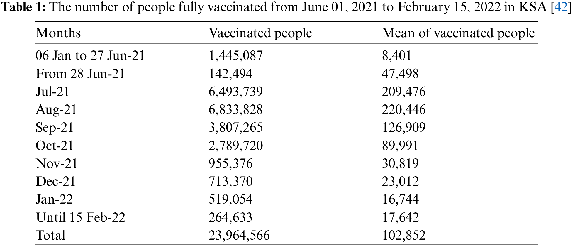
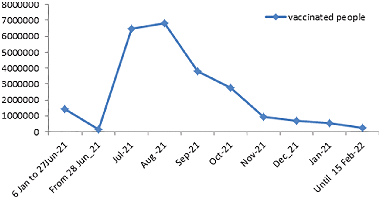
Figure 1: Number of people fully vaccinated in the KSA during the period June 01, 2021 to February 15, 2022
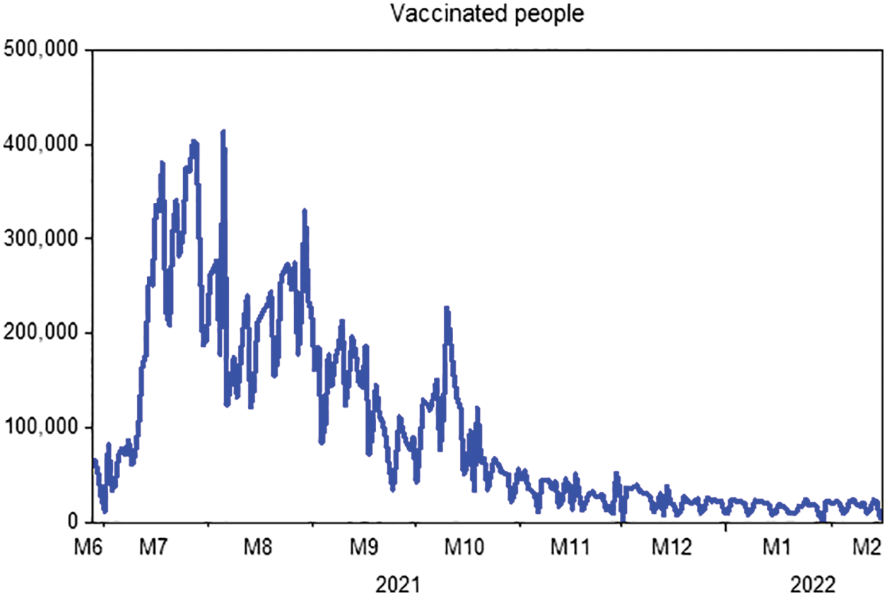
Figure 2: Daily numbers of people completed vaccinations in KSA from June 28, 2021 to February 15, 2022
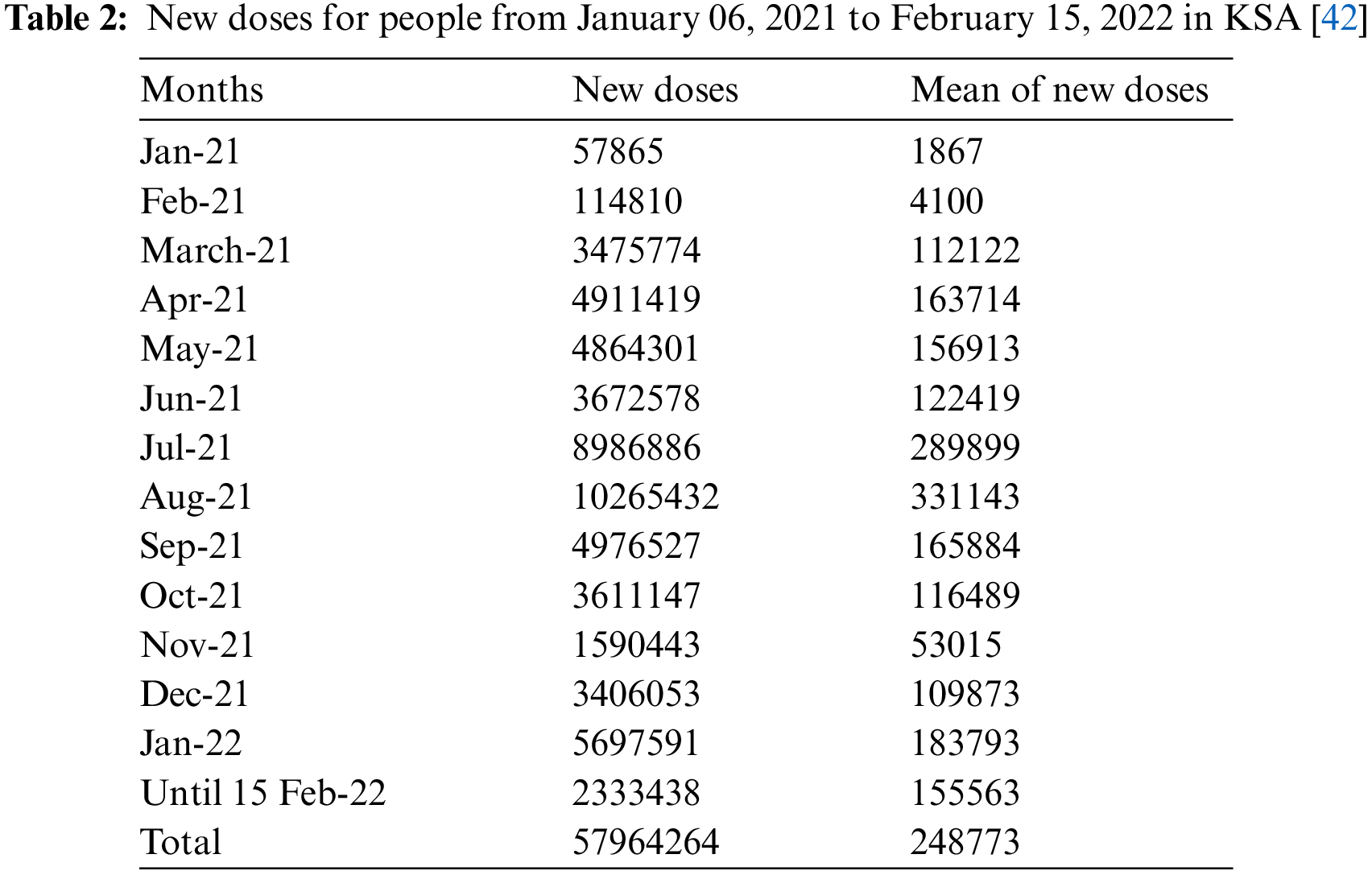
Table 2 summarizes the number of daily doses taken by people against coronavirus disease in KSA during the period June 28, 2021, to February 15, 2022. We find that the doses increased continuously from January 2021 to April 2021, then decreased in May 2021 and June 2021. After that, it increased dramatically in July 2021 and August 2021 to reach 19,252,318 doses with 33% of the total doses given during the study period. Then it decreased during the period from September 2021 to December 2021. The total doses given amounted to 57,964,264 during the studied period, with an average of 248,773 doses per day.
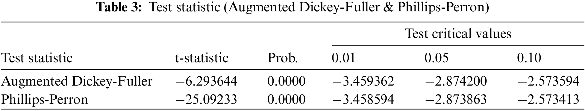
In this portion, we are collecting data on the fully vaccinated people in KSA for the period June 01, 2021 to February 15, 2022. Moreover, the stability tests of these data are examined to use the prediction process as unit root tests and estimation of coefficients (ACF & APCF). Phillips-Peron’s and Dickey-Fuller’s tests show that the data series is unstable at the level, which means that there is a general trend in the series. As shown in Fig. 2. In this regard, we process the data by converting it to the logarithm and taking the first differences to remove the effect of the general trend from the series to be used in estimation and prediction, see Fig. 3. Furthermore, we repeat the unit root tests as in Table 3. Hence, we find that the calculated values are more significant than the critical values and Prob. = 0.0000, which is less than 5%, this indicates that the data series does not have a unit root and has become stable.
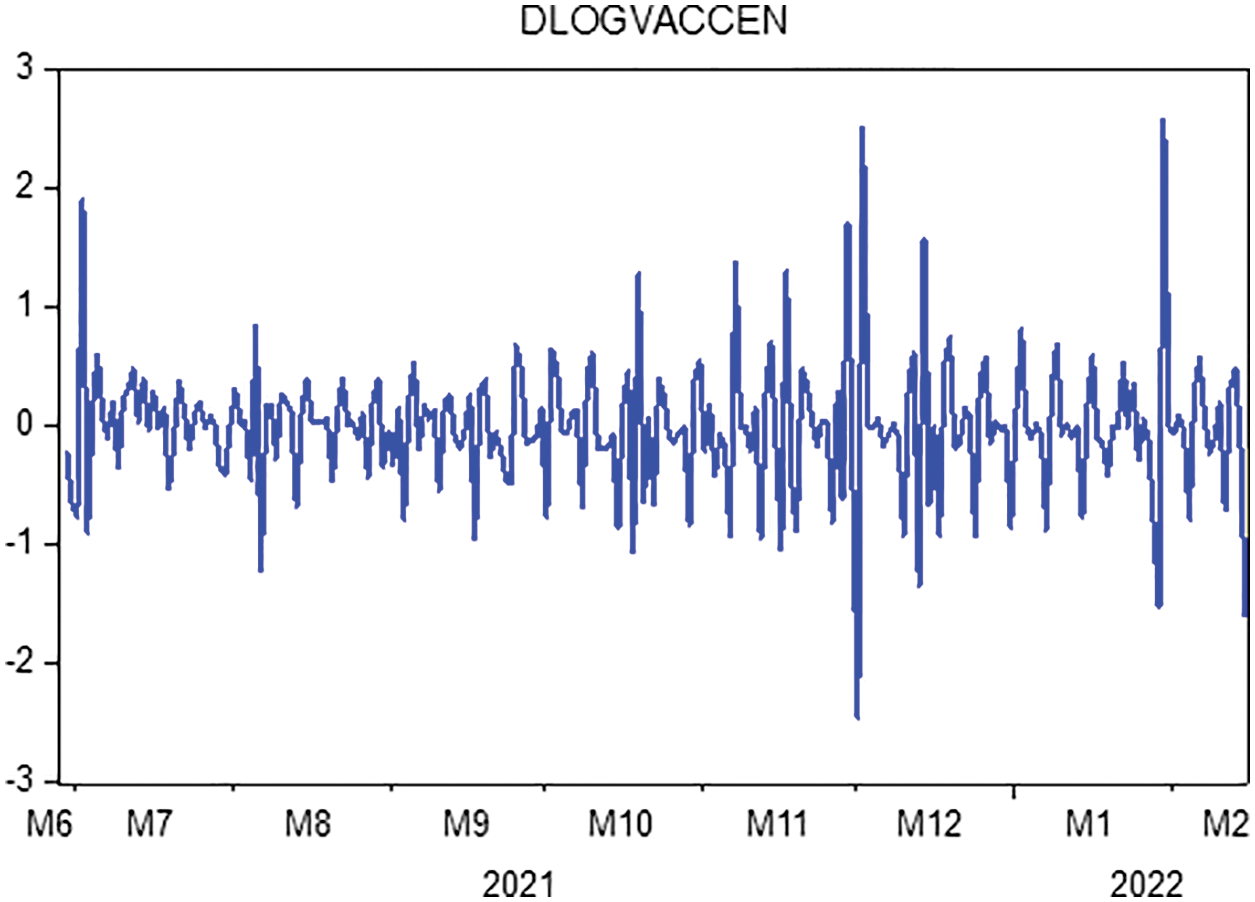
Figure 3: Transformation of the data of completely vaccinated people in KSA to the first difference
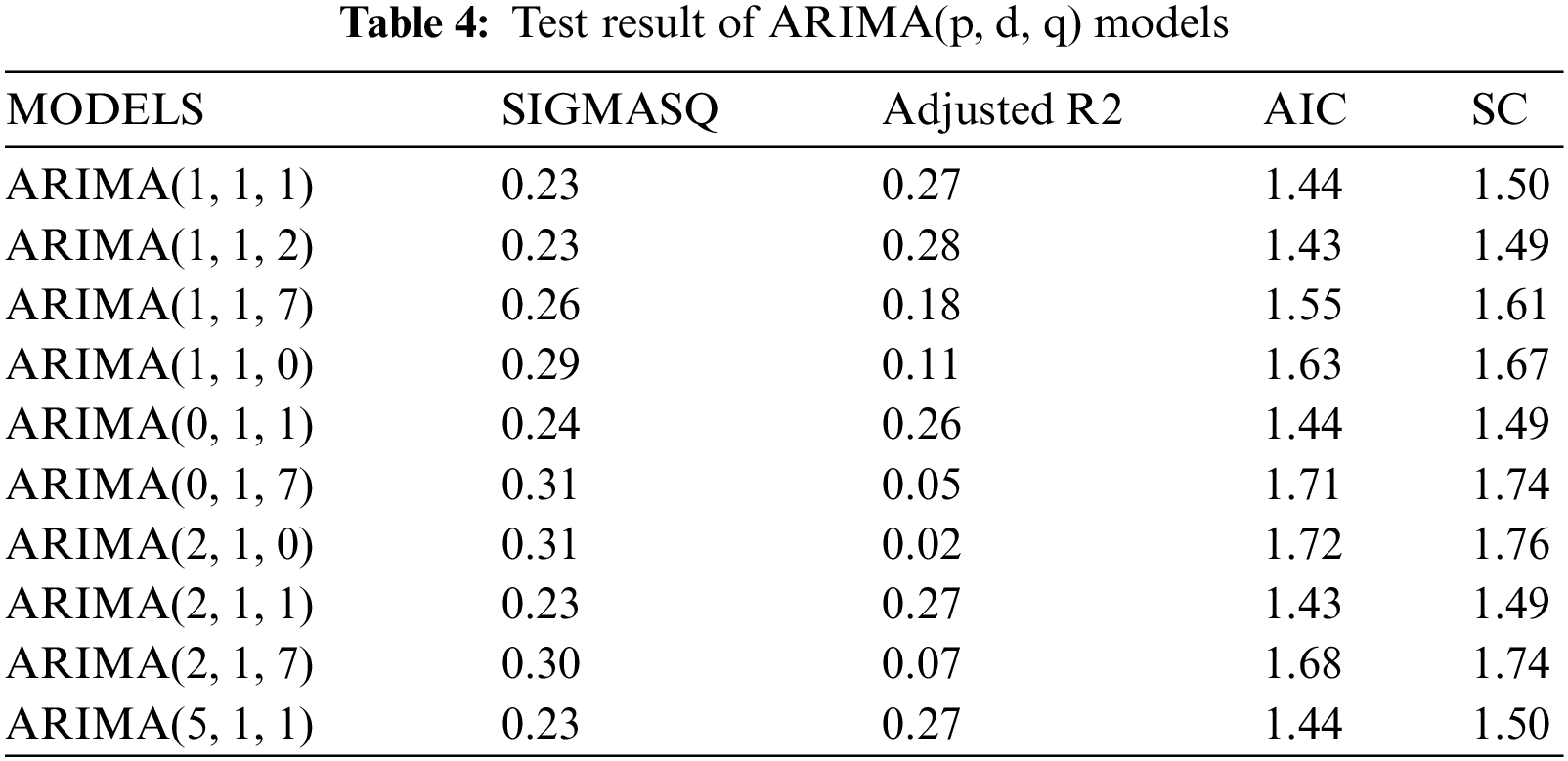
We apply ARIMA models for forecasting through the Eviews program on the data series about the number of vaccinated people completely in KSA. As well, we estimate ARIMA models by using the Ordinary Least Squares method, as shown in Table 4. On the other hand, the models that have no statistical significance are excluded and the comparison only in the statistically significant models, and we are choosing a proper model that achieves the best models in which the coefficient of determination is greater, less variance, less volatility, and less value to AIC indicator.
Moreover, we check the ARIMA (1, 1, 2) model by testing residuals and the shape of the autocorrelation and partial autocorrelation coefficients. It follows from Fig. 4 that the actual values match the estimated values, and this indicates that the differences were small, as well as the efficiency of the model and its suitability in the forecasting process.
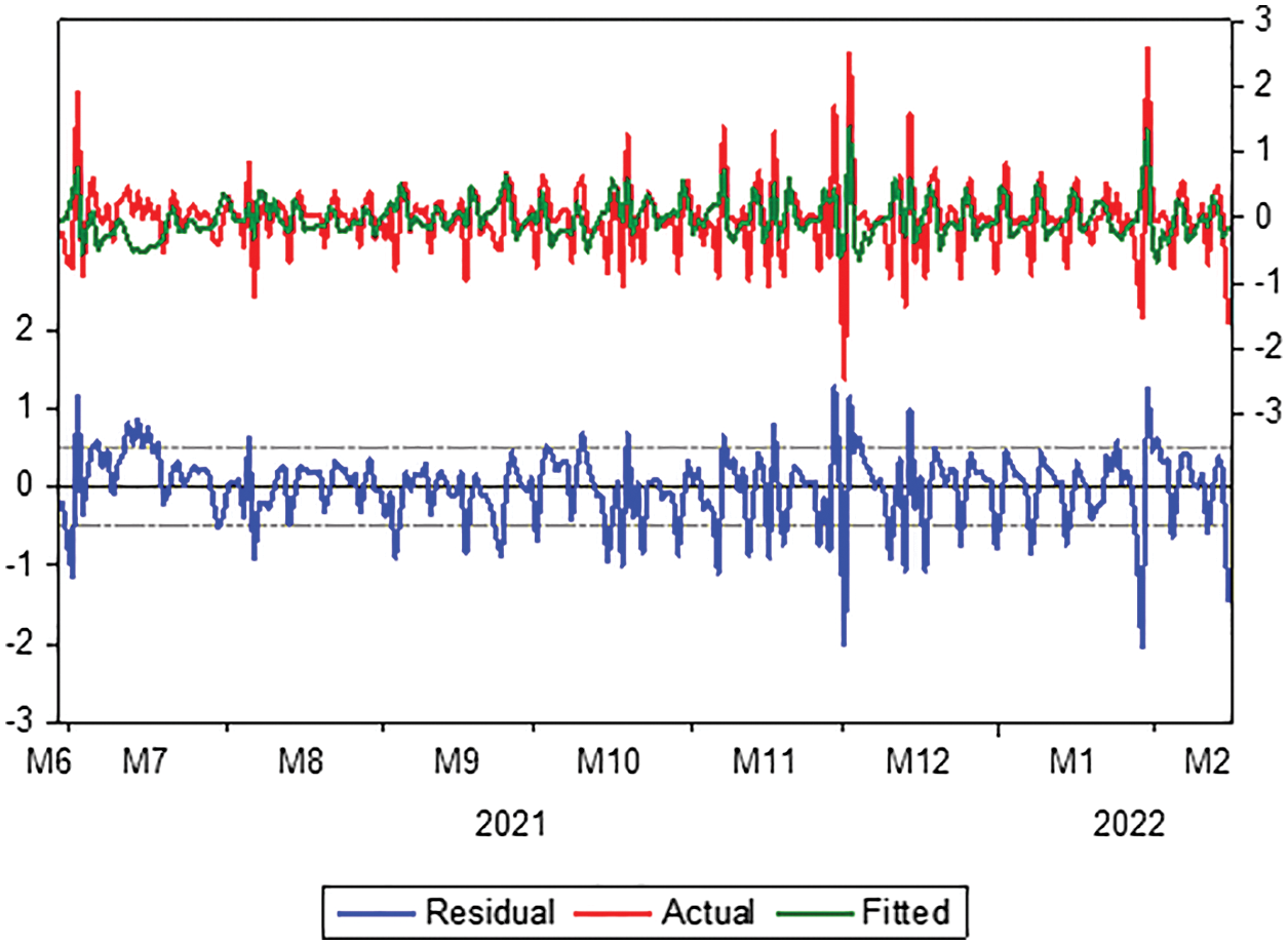
Figure 4: Evaluation of the ARIMA model for actual and fitted values and residual limits
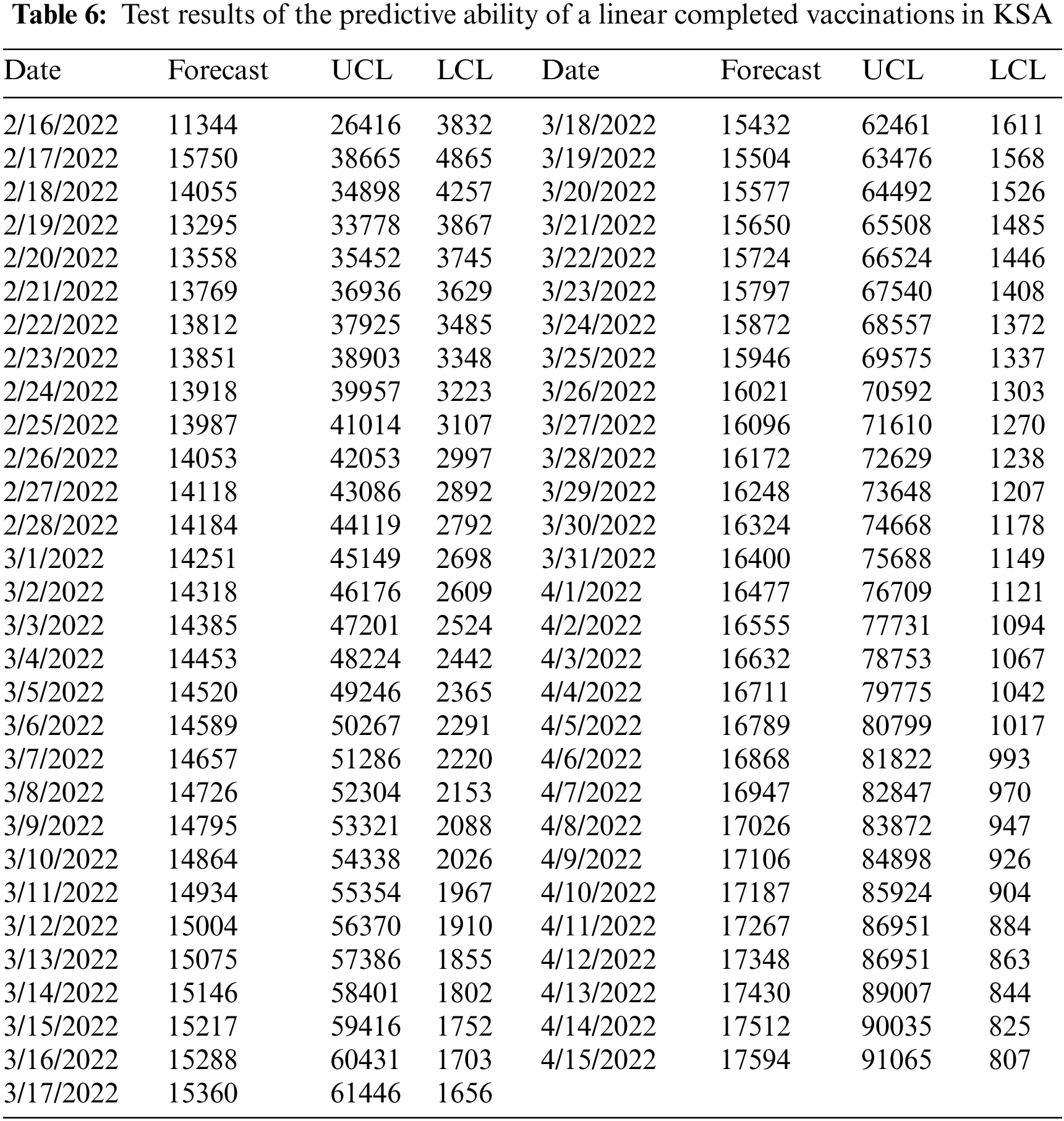
We see through the chosen model a decrease in the number of people who will be fully dosed to (927164) during the predictive period from February 16, 2022, to April 14, 2022. For more details, see Fig. 5 and Table 6.
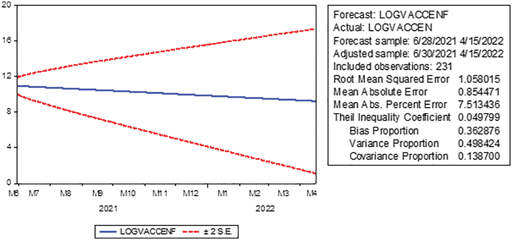
Figure 5: Prediction of the number of fully vaccinated people in KSA with confidence intervals (95%) for the period February 16, 2022 to April 15, 2022
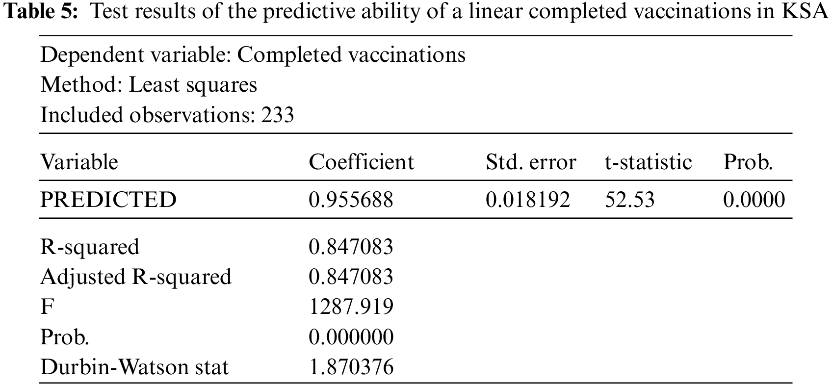
Finally, we estimate a linear model using the least-squares method to test the predictive ability of the model. Indeed, we take the actual values as a dependent variable and the estimated values as an independent variable. We conclude that the closer the estimated parameter to one, the more closely the estimated values are to the actual values. Through the results of Table 5, it is clear that the predicted parameter is close to one (0.955688), and this indicates the quality of the model in prediction and that there is a convergence of the predicted values from the actual values and is statistically significant. Additionally, we find that the value of F = 1287.919, whereas Prob. = 0.0000 is less than 0.05, which indicates the model is significant and good.
Definition 3.1. [20] Let
The normalization function
Definition 3.2. [20] The correspondent AB fractional integral is given by
Lemma 3.1. [22] Let
Lemma 3.2. [20] The Laplace transform of the ABC fractional derivative is defined by
Lemma 3.3. [20] The fractional differential system
4 Model Derivation in ABC Operator
Yavuz et al. [41] developed a mathematical model to reveal the effects of vaccine treatment on COVID-19 described by a system of ODEs as follows:
With initial conditions
In the present work, we make extend the model (2) by replacing the time derivative with the ABC fractional derivative. With this alteration, the right-and left-hand sides will not have the same dimensions. To conquer this affair, we add an auxiliary parameter
With initial conditions
where
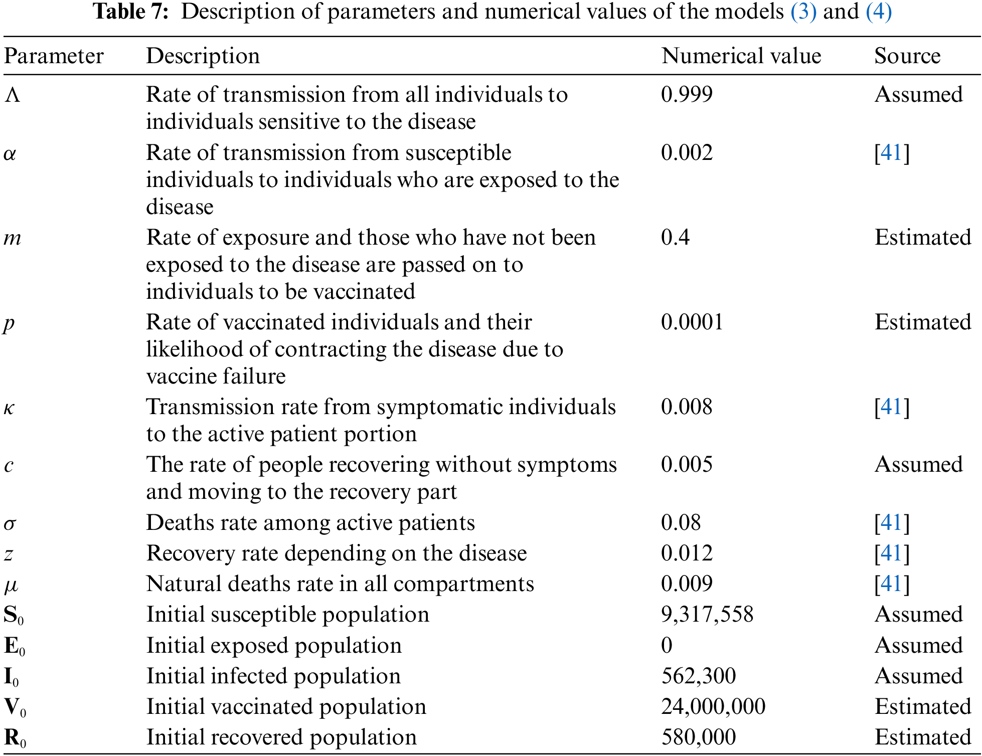
Here S(ϰ) is the class of Susceptible Individuals, E(ϰ) is the class of Exposed Individuals, I(ϰ) is the class of Infected individuals, V(ϰ) is the class of Individuals Vaccinated, R(ϰ) is the class of Recovered Individuals. The model parameter values and source are given in Table 7.
Total population at time ϰ, denoted by N(ϰ) and given by N(ϰ) = S(ϰ) + E(ϰ) + I(ϰ) + V(ϰ) + R(ϰ).
4.1 Positivity and Boundedness
In this portion, we show that the non-negative domain
Theorem 4.1. There is a unique solution
Proof. From the model (3), we have
The norm and all assumptions of the classical results are valid. It follows that:
For
This shows that if
It follows for the whole population that
which implies that
After applying the Laplace transform, we have
where
where
4.2 Equilibrium Points and Reproduction Number
In this part, we will find the equilibrium points of the COVID-19 model. By equating each equation of model (3) to the zero, we can write
For
Hence, the disease free equilibrium (DFE) and endemic equilibrium (EE) are given by the following theorem.
Theorem 4.2. We have the next affirmations:
i. The model (3) has always DFE,
ii. The model (3) has EE,
By using the model (3) and next generation matrix method, the basic reproduction number
For details, see [41].
Stability analysis of the equilibrium points is clarified in [41], exhaustively. In order of stability, the authors dealt with the next two theorems.
Theorem 4.3. The DFE point
Theorem 4.4. The EE point
Here we comment that
In this section, we apply the Picard-Lindel method and the Laplace transform to investigate the existence and uniqueness of solution for preventive and curative to fractional COVID-19 disease model.
5.1 Iterative Scheme with Laplace Transform
Theorem 5.1. For
has a unique solution, which is
Proof. Applying the Laplace transform on both sides of Eq. (5) we obtain
It follows from Theorem 3 in [20] that
which is equivalent to
Applying the inverse Laplace transform give us
Now, we have
Let
Hence
By using Theorem 5.1, our model is equivalent to
The iterative scheme of the model (7) is given by
Taking the limit as
5.2 Existence of a Unique Solution
In this portion, we apply the Picard-Lindel method to investigate the existence of solution for the fractional COVID-19 disease model, which its mathematical represente are presented by:
For sake of simpilicity, we define the functions
The model described in Eq. (9) becomes in the following form:
By applying the operator
The kernels in Eq. (10) satisfies the Lipschitz condition for
where
Repeating the same procedure as in Eq. (13), we get
where
Eq. (12) can be written in the recursive form given by
Now, we denote the difference between successive components by
Taking into account that
Then, we take the norm on both sides of Eq. (17). It follows from Eqs. (14) and (15) that
Next, we shall prove the main theorem based on the above results.
Theorem 5.2. The fractional models (3)--(4) has a unique solution for ϰ ∈ [0, T] if
Proof. Since S(t), E(t), I(t), V(t), and R(t) are bounded functions and satisfying the Lipschitz condition. Therefore, by virtue of Eq. (19), we obtain
Consequently, the sequences in Eq. (21) are exist and smooth, i.e.,
Now, we show that the functions in Eq. (21) are the solutions of the proposed model. We suppose
Then we show that the terms in Eq. (22) verify that
Repeating the procedure above, we get
As
To prove the uniqueness result, we assume that the model (3) has another solution
which implies
It is clear that
This is satisfied by the hypothesis (20). Hence,
Similarly, we obtain
This section gives the numerical solution of the COVID-19 model (3) under ABC fractional derivatives. The suggested fractional model is addressed numerically using a generalized Adams–Bashforth–Moulton technique [44,45].
By applying the operator
For
Over
which implies
Set
Finally,
In an analogous manner for the remainder of the equations of the model (3), we obtain the recursive formulae as below:
The biological parameters estimated from the actual data reported in KSA for the period June 01, 2021 to February 15, 2022, and classified in Table 7 is used to acquire the simulation results. Further for initial data we use S(0) = 9.317558 millions, E(0) = 0, I(0) = 0.562300 million, V(0) = 24.000000 millions, R(0) = 0.580000 million, where N = 34.810000 millions is a total population. For the purposes of numerical simulations, the high estimate of 24,000,000 vaccinated population is considered to account for any uncertainty in the estimate for the current total number of vaccinated individuals population in KSA. We simulate the results for the given 300 days as in Figs. 6–10.
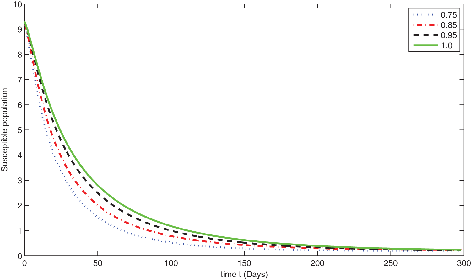
Figure 6: Graphical presentation for different fractional order of the susceptible class for the considered model
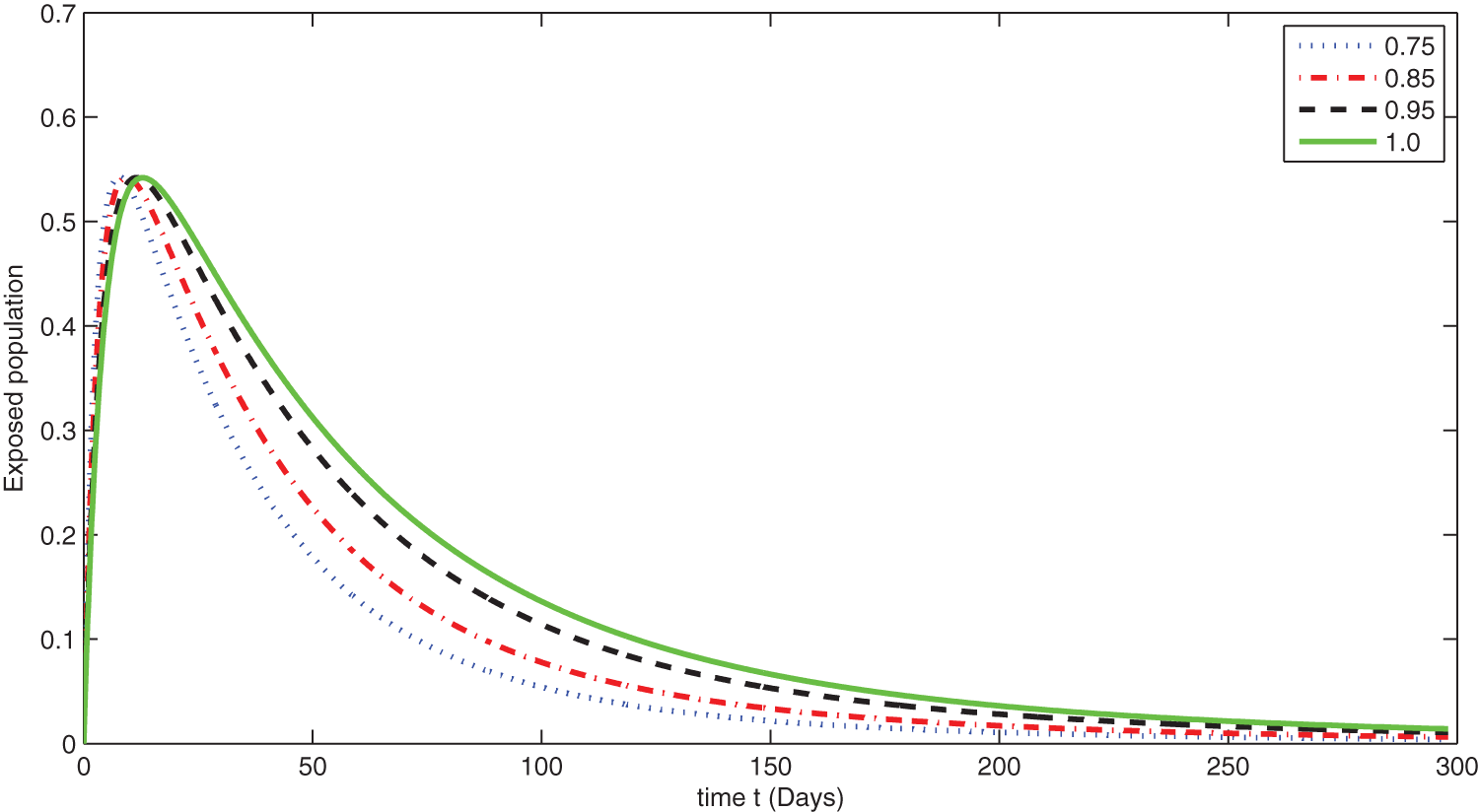
Figure 7: Graphical presentation for different fractional order of the exposed class for the considered model
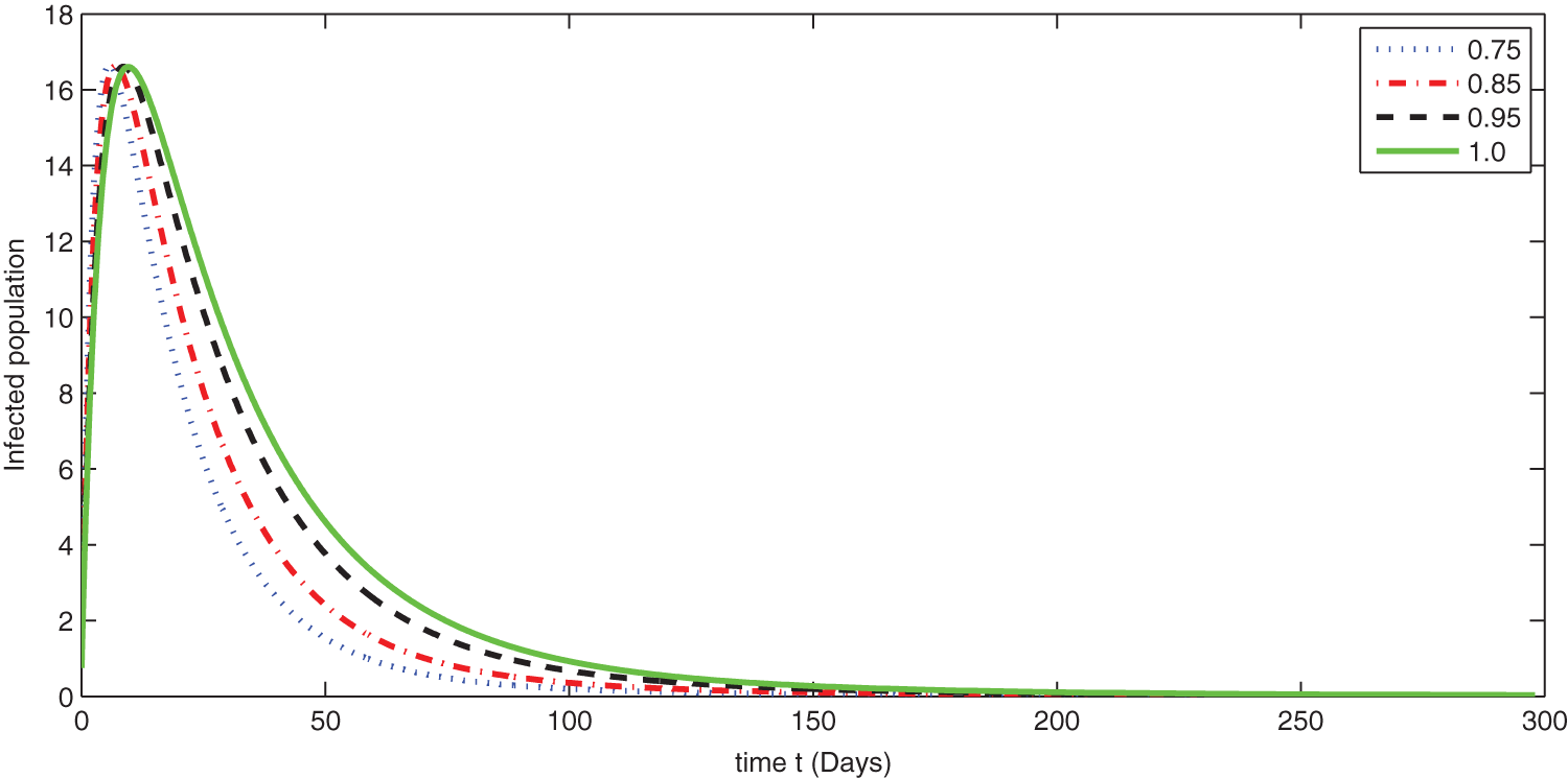
Figure 8: Graphical presentation for different fractional order of the infected class for the considered model
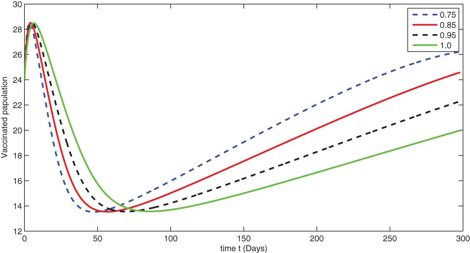
Figure 9: Graphical presentation for different fractional order of the vaccinated class for the considered model
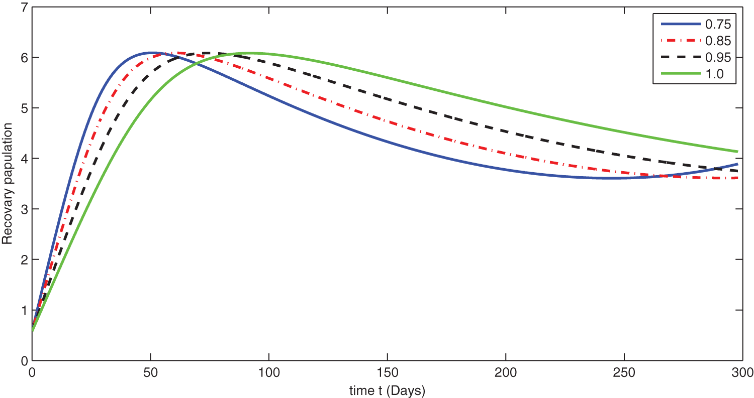
Figure 10: Graphical presentation for different fractional order of the recovered class for the considered model
We see that corresponding to different fractional order, the susceptible class is decreasing with various scenario in Fig. 6. Consequently the density of exposed class is also behave like susceptible at various fractional order, see Fig. 7. The infected class first increase then starts to decline (see Fig. 8) due to vaccination process until become stable as in Fig. 9. Thanking to vaccination the decline in infection will cause the increase in recovery class whose dynamics shows variation due to different fractional order as in Fig. 10. From these graphical presentations we observe the transmission dynamics in the presence of vaccine by using fractional order derivative. The fractional calculus helps us in better understanding of the transmission dynamics in a locality. Also the impact of vaccine is importance which understand from the recovery class presentation. Next, we compared the simulated plots of the population have been fully vaccinated in Fig. 11 with the graphs at different fractional order. We see that graphs are closely agreed which demonstrates the efficiency of our proposed model.
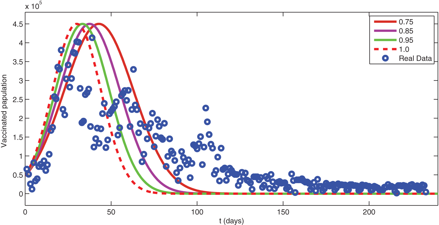
Figure 11: Comparison of real data with different fractional order simulation
In this research work, we have updated a COVID-19 model to a fractional order derivative of generalized type. On the statistical aspect, we have used some statistical analysis to collect data on vaccination in KSA for 300 days, and then the concerned statistical analysis has been shown. Consequently, the forecast about the evolution of the COVID-19 vaccination in 60 days has been presented. We have found, through the ARIMA(1, 1, 2) model, a decrease in the number of people who have been given full doses with (927164), and they constitute 2.6% of the total population in KSA. Data analysis showed that 67.81% of the population had been fully vaccinated during the study period. On the analytical aspect, we have established some adequate results for the existence and uniqueness of the solution through fixed point techniques. The respective results are important because a mathematical formulation should be preferentially checked for their existence. Finally, in terms of numerical aspects, we have extended the Adam-Bashforth method for the considered model to derive a scheme for numerical analysis. Moreover, we have then used the real data for parameters and some initial data of KSA to see the transmission dynamics of COVID-19 with the vaccinated class. Finally, the concerned numerical simulations have been compared with the exact real available date given in Section 2. We see that the real data plot and simulated data plots coincide very well. This phenomenon demonstrates the applicability of the method.
Authors’ Contributions: All authors contributed equally and significantly in writing this paper. All authors read and approved the final manuscript.
Acknowledgement: The authors would like to thank Imam Mohammad Ibn Saud Islamic University (IMSIU), for funding this research work.
Data Availability Statement: Data are available upon request.
Funding Statement: This research was supported by the Deanship of Scientific Research, Imam Mohammad Ibn Saud Islamic University (IMSIU), Saudi Arabia, Grant No. (21-13-18-069).
Conflicts of Interest: The authors declare that they have no conflicts of interest to report regarding the present study.
References
1. Hu, B., Guo, H., Zhou, P., Shi, Z. L. (2021). Characteristics of SARS-CoV-2 and COVID-19. Nature Reviews Microbiology, 19, 141–154. DOI 10.1038/s41579-020-00459-7. [Google Scholar] [CrossRef]
2. WHO (2021). World Health Organization Weakly Report. https://www.who.int/emergencies/diseases/novel-coronavirus-2019. [Google Scholar]
3. Worldometers.info (2021). Coronavirus cases-worldometer. https://www.worldometers.info/coronavirus. [Google Scholar]
4. FDA, U.S. FOOD & DRUG. COVID-19 Vaccines (2022). https://www.fda.gov/emergency-preparedness-and-response/coronavirus-disease-2019-covid-19/covid-19-vaccines. [Google Scholar]
5. Mathevet, T., Lepiller, M., Mangin, A. (2004). Application of time series analyses to the hydrological functioning of an alpine karstic system: The case of Bange-L’Eua-Morte. Hydrology and Earth System Sciences, 8(6), 1051–1064. DOI 10.5194/hess-8-1051-2004. [Google Scholar] [CrossRef]
6. Khan, F., Pilz, J. (2018). Modelling and sensitivity analysis of river flow in the upper Indus basin: Pakistan. International Journal of Water, 12(1), 1–21. DOI 10.1504/IJW.2018.090184. [Google Scholar] [CrossRef]
7. Box, G., Jenkins, G. (1970). Time series analysis, forecasting and control. San Francisco: Holden-Day. [Google Scholar]
8. Maleki, M., Mahmoudi, M. R., Wraith, D., Pho, K. H. (2020). Time series modelling to forecast the confirmed and recovered cases of COVID-19. Travel Medicine and Infectious Disease, 37, 101742. DOI 10.1016/j.tmaid.2020.101742. [Google Scholar] [CrossRef]
9. Podlubny, I. (1999). Fractional differential equations. San Diego: Academic Press. [Google Scholar]
10. Samko, S. G., Kilbas, A. A., Marichev, O. I. (1993). Fractional integrals and derivatives. Yverdon: Gordon & Breach. [Google Scholar]
11. Kilbas, A. A., Srivastava, H. M., Trujillo, J. J. (2006). Theory and applications of fractional differential equations. Amsterdam: North-Holland Mathematics Studies, Elsevier. [Google Scholar]
12. Ross, B. (2006). A brief history and exposition of the fundamental theory of fractional calculus. Fractional Calculus and Its Applications, 457, 1–36. DOI 10.1007/BFb0067096. [Google Scholar] [CrossRef]
13. Yang, X. J. (2019). General fractional derivatives: Theory, methods and applications. Chapman and Hall/CRC. DOI 10.1201/9780429284083. [Google Scholar] [CrossRef]
14. Toufik, M., Atangana, A. (2017). New numerical approximation of fractional derivative with non-local and non-singular kernel: Application to chaotic models. The European Physical Journal Plus, 132(10), 1–16. [Google Scholar]
15. Koca, I. (2018). Modelling the spread of Ebola virus with Atangana-Baleanu fractional operators. The European Physical Journal Plus, 133(3), 100. DOI 10.1140/epjp/i2018-11949-4. [Google Scholar] [CrossRef]
16. Atangana, A., Gomez-Aguilar, J. F. (2018). Decolonisation of fractional calculus rules: Breaking commutativity and associativity to capture more natural phenomena. The European Physical Journal Plus, 133(4), 166. DOI 10.1140/epjp/i2018-12021-3. [Google Scholar] [CrossRef]
17. Tateishi, A. A., Ribeiro, H. V., Lenzi, E. K. (2017). The role of fractional time-derivative operators on anomalous diffusion. Frontiers in Physics, 52(5), 19. DOI 10.3389/fphy.2017.00052. [Google Scholar] [CrossRef]
18. Caputo, M., Fabrizio, M. (2015). A new definition of fractional derivative without singular kernel. Progress in Fractional Differentiation and Applications, 1(2), 73–85. [Google Scholar]
19. Losada, J., Nieto, J. J. (2015). Properties of a new fractional derivative without singular kernel. Progress in Fractional Differentiation and Applications, 1(2), 87–92. [Google Scholar]
20. Atangana, A., Baleanu, D. (2016). New fractional derivative with non-local and non-singular kernel. Thermal Science, 20(2), 757–763. DOI 10.2298/TSCI160111018A. [Google Scholar] [CrossRef]
21. Jarad, F., Abdeljawad, T., Hammouch, Z. (2018). On a class of ordinary differential equations in the frame of Atangana-Baleanu fractional derivative. Chaos Solitons Fractals, 117, 16–20. DOI 10.1016/j.chaos.2018.10.006. [Google Scholar] [CrossRef]
22. Abdeljawad, T. (2017). A Lyapunov type inequality for fractional operators with nonsingular Mittag-Leffler kernel. Journal of Inequalities and Applications, 2017(1), 130. DOI 10.1186/s13660-017-1400-5. [Google Scholar] [CrossRef]
23. Atangana, A. (2018). Non validity of index law in fractional calculus: A fractional differential operator with Markovian and non-Markovian properties. Physica A: Statistical Mechanics and Its Applications, 505, 688–706. DOI 10.1016/j.physa.2018.03.056. [Google Scholar] [CrossRef]
24. Atangana, A., Gomez-Aguilar, J. F. (2018). Fractional derivatives with no-index law property: Application to chaos and statistics. Chaos Solitons Fractals, 114, 516–535. DOI 10.1016/j.chaos.2018.07.033. [Google Scholar] [CrossRef]
25. Abdo, M. S., Shah, K., Wahash, H. A., Panchal, S. K. (2020). On a comprehensive model of the novel coronavirus (COVID-19) under Mittag-Leffler derivative. Chaos Solitons Fractals, 135, 109867. DOI 10.1016/j.chaos.2020.109867. [Google Scholar] [CrossRef]
26. Almalahi, M. A., Panchal, S. K., Shatanawi, W., Abdo, M. S., Shah, K. et al. (2021). Analytical study of transmission dynamics of 2019-nCoV pandemic via fractal fractional operator. Results in Physics, 24, 104045. DOI 10.1016/j.rinp.2021.104045. [Google Scholar] [CrossRef]
27. Jeelani, M. B., Alnahdi, A. S., Abdo, M. S., Abdulwasaa, M. A., Shah, K. et al. (2021). Mathematical modeling and forecasting of COVID-19 in Saudi Arabia under fractal-fractional derivative in caputo sense with power-law. Axioms, 10(3), 228. DOI 10.3390/axioms10030228. [Google Scholar] [CrossRef]
28. Abdulwasaa, M. A., Abdo, M. S., Shah, K., Nofal, T. A., Panchal, S. K. et al. (2021). Fractal-fractional mathematical modeling and forecasting of new cases and deaths of COVID-19 epidemic outbreaks in India. Results in Physics, 20, 103702. DOI 10.1016/j.rinp.2020.103702. [Google Scholar] [CrossRef]
29. Atangana, A. (2020). Modelling the spread of COVID-19 with new fractal-fractional operators: Can the lockdown save mankind before vaccination. Chaos Solitons Fractals, 136, 109860. DOI 10.1016/j.chaos.2020.109860. [Google Scholar] [CrossRef]
30. Zhang, Z. (2020). A novel COVID-19 mathematical model with fractional derivatives: Singular and nonsingular kernels. Chaos Solitons Fractals, 139, 110060. DOI 10.1016/j.chaos.2020.110060. [Google Scholar] [CrossRef]
31. Khan, A., Alshehri, H. M., Abdeljawad, T., Al-Mdallal, Q. M., Khan, H. (2021). Stability analysis of fractional nabla difference COVID-19 model. Results in Physics, 22, 103888. DOI 10.1016/j.rinp.2021.103888. [Google Scholar] [CrossRef]
32. Khan, Z. A., Khan, A., Abdeljawad, T., Khan, H. (2022). Computational analysis of fractional order imperfect testing infection disease model. Fractals. DOI 10.1142/S0218348X22401697. [Google Scholar] [CrossRef]
33. Ullah, I., Ahmad, S., Al-Mdallal, Q., Khan, Z. A., Khan, H. et al. (2020). Stability analysis of a dynamical model of tuberculosis with incomplete treatment. Advances in Difference Equations, 2020, 499. DOI 10.1186/s13662-020-02950-0. [Google Scholar] [CrossRef]
34. Shah, K., Khan, Z. A., Ali, A., Amin, R., Khan, H. et al. (2020). Haar wavelet collocation approach for the solution of fractional order COVID-19 model using caputo derivative. Alexandria Engineering Journal, 59(5), 3221–3231. DOI 10.1016/j.aej.2020.08.028. [Google Scholar] [CrossRef]
35. Habenom, H., Aychluh, M., Suthar, D. L., Al-Mdallal, Q., Purohit, S. D. (2022). Modeling and analysis on the transmission of COVID-19 pandemic in Ethiopia. Alexandria Engineering Journal, 61(7), 5323–5342. DOI 10.1016/j.aej.2021.10.054. [Google Scholar] [CrossRef]
36. Bozkurt, F., Yousef, A., Abdeljawad, T., Kalinli, A., Al Mdallal, Q. (2021). A fractional-order model of COVID-19 considering the fear effect of the media and social networks on the community. Chaos Solitons Fractals, 152, 111403. DOI 10.1016/j.chaos.2021.111403. [Google Scholar] [CrossRef]
37. Sindhu, T. N., Shafiq, A., Al-Mdallal, Q. M. (2021). On the analysis of number of deaths due to COVID-19 outbreak data using a new class of distributions. Results in Physics, 21, 103747. DOI 10.1016/j.rinp.2020.103747. [Google Scholar] [CrossRef]
38. Shafiq, A., Lone, S. A., Sindhu, T. N., El Khatib, Y., Al-Mdallal, Q. M. et al. (2021). A new modified kies Fréchet distribution: Applications of mortality rate of COVID-19. Results in Physics, 28, 104638. DOI 10.1016/j.rinp.2021.104638. [Google Scholar] [CrossRef]
39. Diagne, M. L., Rwezaura, H., Tchoumi, S. Y., Tchuenche, J. M. (2021). A mathematical model of COVID-19 with vaccination and treatment. Computational and Mathematical Methods in Medicine, 2021, 1250129. DOI 10.1155/2021/1250129. [Google Scholar] [CrossRef]
40. Gokbulut, N., Kaymakamzade, B., Sanlidag, T., Hincal, E. (2021). Mathematical modelling of COVID-19 with the effect of vaccine. AIP Conference Proceedings, 2325(1), 020065. DOI 10.1063/5.0040301. [Google Scholar] [CrossRef]
41. Yavuz, M., CoşarÖ, F., Günay, F., Özdemir, F. N. (2021). A new mathematical modeling of the COVID-19 pandemic including the vaccination campaign. Open Journal of Modelling and Simulation, 9(3), 299–321. DOI 10.4236/ojmsi.2021.93020. [Google Scholar] [CrossRef]
42. covidvax.live (2021). http://covidvax.live/ar/location/sau. [Google Scholar]
43. Gómez-Aguilar, J. F., Rosales-García, J. J., Bernal-Alvarado, J. J., Córdova-Fraga, T., Guzmán-Cabrera, R. (2012). Fractional mechanical oscillators. Revista Mexicana de Física, 58(4), 348–352. [Google Scholar]
44. Toufik, M., Atangana, A. (2017). New numerical approximation of fractional derivative with non-local and non-singular kernel: Application to chaotic models. Chaos Solitons Fractals, 132, 444. DOI 10.1140/epjp/i2017-11717-0. [Google Scholar] [CrossRef]
45. Diethelm, K., Freed, A. D. (1998). The FracPECE subroutine for the numerical solution of differential equations of fractional order. Forschung und Wissenschaftliches Rechnen, 1999, 57–71. [Google Scholar]
Cite This Article
 Copyright © 2023 The Author(s). Published by Tech Science Press.
This work is licensed under a Creative Commons Attribution 4.0 International License , which permits unrestricted use, distribution, and reproduction in any medium, provided the original work is properly cited.
 Downloads
 Citation Tools