An Interpretable CNN for the Segmentation of the Left Ventricle in Cardiac MRI by Real-Time Visualization

1  Introduction

Cardiovascular disease remains the top cause of global mortality, with more people dying yearly than from any other reason. It has become a major public health issue. Coronary heart disease affects the left ventricle region of the heart primarily. Estimating left ventricular function parameters using left ventricular segmentation images can aid doctors in diagnosing the disease. Because doctors spend much of their time and energy manually segmenting the left ventricle, using algorithms to do so automatically will greatly improve the doctor’s effectiveness.

There are various important deep learning applications for image analysis that should divide the image into spatial zones of interest rather than detecting individual items within a zone. According to medical image analysis, the pixels corresponding to distinct types of tissue, blood, and abnormal cells should be differentiable so that a particular organ can be isolated. Because of the complexity of medical images, a number of issues (e.g., local variations and non-uniformity) must be addressed throughout the segmentation process, making direct use of general image segmentation methods impossible. Semantic segmentation aims to assign each pixel to a given class. This is a classification problem; this study was based on individual pixels rather than on an entire image.

Medical imaging can help doctors with clinical diagnoses but telling doctors whether an MRI image is of the left ventricle is insufficient. Moreover, CNNs are known for their classification and segmentation outputs [1,2]; however, doctors also want to know what the interpretable medical AI is saying and the effect of the respective model layer on the image. In addition, as mobile smartphones and tablets have become ubiquitous and standard office equipment, a growing number of doctors have begun to use them for clinical activities, such as viewing medical images and submitting diagnostic advice. Because mobile devices have limited computing capacity, a lightweight, fast segmentation algorithm is needed. However, current techniques are computationally difficult and need considerable resources.

To meet these needs, this study developed a model with optimized size and parameters suitable for a doctor’s use. It could verify hypotheses. Through model visualization, doctors can participate directly in the evolution of the model and assist data scientists in improving performance. This study aims to make common deep learning activities easier, including data management, neural network design, training on multi-GPU systems, and real-time performance monitoring with enhanced visualizations. Selecting the optimal model from the results browser for deployment was also an aim. Data scientists can focus on designing and training networks rather than on complex programming and debugging. In addition, this model is more suitable for deployment on mobile devices.

We struck a balance between algorithm complexity, processing time, and segmentation accuracy and found that lightweight models could perform comparably to ImageNet architectures and be applied to mobile devices. The remainder of this paper is arranged as follows. Section 3 proposes an explainable model—explainable methods are provided before modeling, explainable mode methods are established, and an explanation is provided after modeling the methods. Section 4 evaluates the performance. At the end, Section 5 presents a discussion and draws conclusions. The contributions of this study are presented below:

•   We did not depend on transfer learning or a pretrained model; we designed a multi-convolution stack model using the interpretable modeling approach (i.e., first is interpretability before modeling, then establishing a model that can be explained and, finally, explaining the model output).

•   We used an explainable global average pooling layer to replace the fully connected layers. Global average pooling can explain and reduce the number of parameters while maintaining satisfactory performance. Overfitting was avoided, and the structure was simple.

•   We enhanced our framework visualizations to improve interpretability. We analyzed the performance per accuracy, loss, and Dice and the features of each layer of the CNN in real-time.

2  Related Work

2.1 Explainable Deep Learning Model

An explainable model is a function that is too difficult for humans to comprehend, also called a black box, which can provide insights into how it operates. To do this, we need an additional method. Samek et al. [3] proposed visual analytics methods [4,5] for explainable deep learning. They highlighted potential problems and future research approaches after reviewing visual analytics, information visualization, and learning perspectives pertinent to this goal. Zhang et al. [6,7] presented a method for converting a traditional convolutional neural network (CNN) into an interpretable CNN to explain knowledge representations in the CNN’s high convolutional layer. Kuo et al. [8] proposed a determination of CNN parameters based on an interpretable feed-forward design methodology.

Since the clinical use of deep learning algorithms has been limited due to their black-box nature, Ghosal et al. [9] provided various approaches. From the perspective of a deep learning scientist tasked with developing a solution for end-users in healthcare, the hurdles for clinical deployment and issues requiring more research were presented. They provided pre-model vs. in-model vs. post-model approaches, for example.

Zheng et al. [10] suggested semi-supervised learning of apparent flow for explainable heart disease categorization using cine-MRI with motion characterization.

2.2 Unexplainable Network

2.2.1 Transfer Learning

In medical image analysis, deep learning-based annotation and segmentation can speed-up model development. However, developing an effective model from scratch is time-consuming and requires that an effective model be developed. This also requires considerable investment and effective datasets. These factors have always been the toughest challenge for developers. In November 2018, NVIDIA launched the Transfer Learning Toolkit (TLT) [11] for medical imaging based on deep learning. Various advanced and complex algorithms in deep learning have become more popular in applying medical images through transfer learning.

Raghu et al. [12] asked why there are only thousands of training samples. They had to assess transfer learning in small data environments. They found that a large model designed for ImageNet has too many parameters for a small amount of data. Using a comprehensive performance review and an analysis of hidden representations of neural networks, they found that transfer learning is limited in improving the performance of tested medical imaging tasks. This performance was unaffected by transfer learning, and a model trained from scratch performed on par with the conventional ImageNet transfer model.

2.2.2 Attention Module

According to the findings of Jain et al. [13], standard attention modules do not provide meaningful explanations and should not be treated as though they do.

The obtained models above make it difficult to explain the relevance or causality between its input and output in clinical practice and lack the process’ interpretability. It is difficult to obtain information supporting causal reasoning for medical diagnosis or research.

2.3 Medical Image Segmentation

Image segmentation has experienced years of development, and many excellent semantic segmentation networks have been proposed (e.g., FCN, U-Net, SegNet, and DeepLab). Wu et al. [14], to accurately segment LVs, built a hybrid model combining CNN and U-Net. However, overfitting proved to be a problem common in deep networks. Affected by many parameters that need to be learned, especially for U-Net, their model needed to use transfer methods. However, medical image segmentation has made substantial use of attention mechanisms. Sinha et al. [15] first used multiscale self-guided attention for medical image segmentation by capturing richer contextual dependencies through the guided self-attention techniques that helped filter out noise to highlight pertinent information. Cai et al. [16] used an attention mechanism to explicitly model the dependencies between channels and mix local features with their equivalent global dependencies. They used multiscale prediction fusion with global information on different scales to eliminate semantic ambiguity in the jump connection operation.

Deep learning algorithms for image segmentation are becoming a promising building block in medical image segmentation. Transfer learning methods and attention modules have been popularized. However, the inexplicability of the black box of deep learning hinders the development of intelligent medical diagnosis. Deep learning models in medical imaging and their interpretability in medical imaging are becoming a research hotspot.

3  Methodology

The complexity of the method, the time required, and the segmentation results, all limitations imposed by the algorithm we choose, are factors to consider. Raghu et al. [12] asserted that transfer learning has no major impact on medical imaging task performance. A model trained from scratch is almost as good as the standard ImageNet transfer model. Thus, unexplainable methods were excluded from designing an explainable model from scratch.

3.1 Interpretation Methods before Modeling

Before modeling [17–20], the interpretation method is a series of strategies with the common purpose of learning more about the datasets used in model construction [5–8]. Machine learning solves the problem of discovering knowledge and rules from data. If the designer knows little about the characteristics of their data, it is unrealistic to expect much understanding of the problem. The importance of interpretable methodologies before modeling is that they assist designers in quickly and thoroughly understanding the properties of data distribution, considering potential issues in the model design procedure and selecting the most appropriate model for approaching the perfect solution.

Medical images are highly complex. The internal structure of the human body is generally constant, with a broad gray scale range and hazy borders. The semantics are complex and intricate, and the distribution of segmentation objectives in these images is regular (e.g., inter-annotator conflicts and poor segmentation reproducibility) [21].

Because medical imaging data collection is difficult and the data available are limited, overfitting in a model is common; so, a tiny model with a limited set of factors is appropriate [22].

Fig. 1 illustrates two datasets. Each image row represents a single instance of the data. On the left is an MRI image, and on the right are areas marked by an expert (often called contours). The sections of the image that are part of the LV are represented by white. The size of the LV depends on the image, but it usually occupies only a small portion of the total image area.

Figure 1: MRI and expert annotation

The photos were originally created in 256 × 256 grayscale DICOM format [1–3]. The contour is a tensor with the dimensions of 256 × 256 × 2.

3.2 Establish an Interpretable Model

The issue with creating explainable AI strategies is that many AI models have important tradeoffs when accuracy and transparency are balanced.

A convolution layer was employed to capture small regions of interest, while a larger receptive field was used to record broader receptive fields. Pooling layers were added, which down sampled the data while attempting to retain most of the information. This eliminated some computational complexity.

Layers typically associated with image recognition neural networks have been described [5,6], where the number of output nodes equaled the number of classes. Each pixel was classified in the image so that the output size would be the number of classes, two. Additionally, the spatial location of the output nodes was important since each pixel had an associated probability of being part of the LV.

CNNs are well-established as excellent choices for image recognition or classification tasks. The task in this study was segmentation, which was related to classification in a sense. Each pixel was classified in the image rather than the entire image altogether. To utilize the same type of CNN already shown to do very well on image recognition for the segmentation task, we must make some modifications to CNN models.

This study used a global average pooling layer. In the global average pooling layer, there was no full connection layer (i.e., no fixed graph size); so, it would be easy to adapt to many input sizes. The following figure depicts how these data change in the following task.

Fig. 2 depicts a CNN consisting of convolution layers, pooling layers, an UnPool, and a combined layer.

Figure 2: Structure of the network

Fig. 3 is prompted by the VGGnet stack of three 3 × 3 convolution layers. Instead of a single 7 × 7 layer, it introduced more nonlinearity (more hidden layers, thereby introducing more nonlinear functions), improved the decision power of the decision function, and introduced fewer parameters.

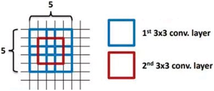
Figure 3: Stack convolution

The average feature for a layer was used to enhance the features at the respective location using global average pooling (GAP). A context vector was created by pooling a layer’s feature map across the entire image. The context vector is normalized to create new feature maps of the same dimensions as the originals. The feature maps above were then concatenated.

According to Fig. 4, the GAP operation could be considered the expectation of obtaining the confidence of the full picture of the respective category. Because there was only a convolutional layer, spatial information was well preserved, and interpretability increased. There was no fully connected layer, which reduced the number of parameters and overfitting to a certain extent.

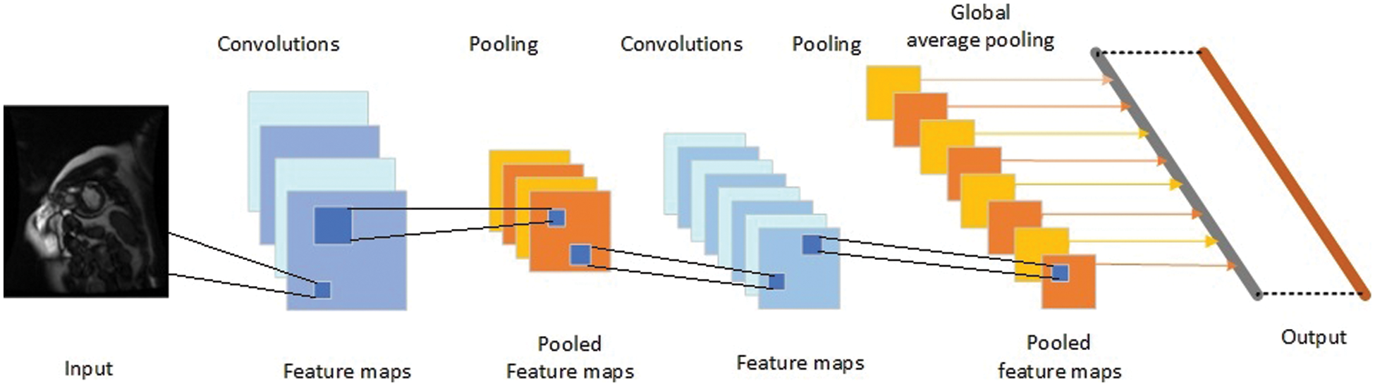
Figure 4: Mechanism of global average pooling

We obtain Sc by entering Fk=∑x,yfk(x,y) into a class score

Sc=∑kωkc∑x,yfk(x,y)=∑x,y∑kωkcfk(x,y).(1)

The class activation map for class c is defined as Mc, where each spatial element is given by

Mc(x,y)=∑kωkcfk(x,y).(2)

Thus, Sc=∑x,yMc(x,y).

3.3 Interpretation after Model Building

This study focused on model visualization [23,24] in this part. After modeling, the interpretable technique primarily strives for a deep learning model with internal features, not visible properties. For neural networks, the number of hidden layers is constantly a metaphysics. The goal of NVIDIA DIGITS [25] is to visualize CNNs to obtain a human-interpretable overview of the hidden network layers’ concepts. This study used the improved NVIDIA DIGITS system to train and analyze the performance of the trained model. During and after the training phase, the designer might see a change in the hidden layer’s performance by analyzing the model’s accuracy. The outcome of the training process was visualized. The developer can monitor the output of image convolution, which aids in the understanding of the convolution kernel’s function. The developer might use the heat map to determine which sections of the image are important in the image classification challenge and find the positions of items in the image.

On the right side of Fig. 5, NVIDIA DIGITS uses a gradient attribution method [26] to generate a pixel-resolution map that shows which pixels are most significant for network classification. This algorithm calculates the class score’s gradient regarding the input pixels. The maps, on the surface, appear to demonstrate which pixels impact the class score most when modified. The left side of Fig. 5 shows the shape, mean, and standard deviation of the data in this layer. The third layer of convolution consists of 384 columns and 256 rows of pixels, the convolution kernel is 3 × 3, and the weights have learned 885,120 parameters through convolution. It also shows that a pixel’s mean and standard deviation are both 0.

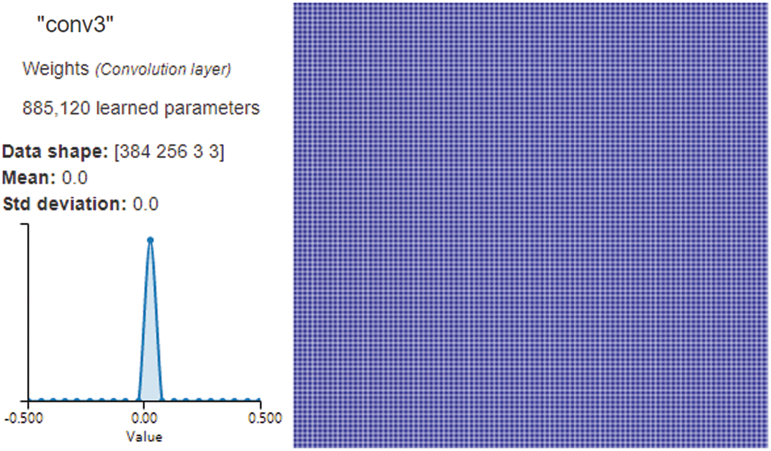
Figure 5: Convolution Layer3 visualization

We enhanced NVIDIA DIGITS by employing class activation maps (CAM) [26] to generate visual interpretations of CNN predictions. CAM uses the GAP layer in the CNN to generate a map highlighting which parts of an image the network uses in relation to a specific class label. According to Fig. 6, we can see which portions of the image are important in the image classification. We could use the GAP layer and the heat map to simultaneously determine where objects are in the image. The red portion of the figure indicates that the model has been placed at the center of the left ventricle, and the cyan edge outlines the left ventricle’s boundary. It assists doctors in understanding how the model recognizes the left ventricle and model developers in determining whether the model is accurate.

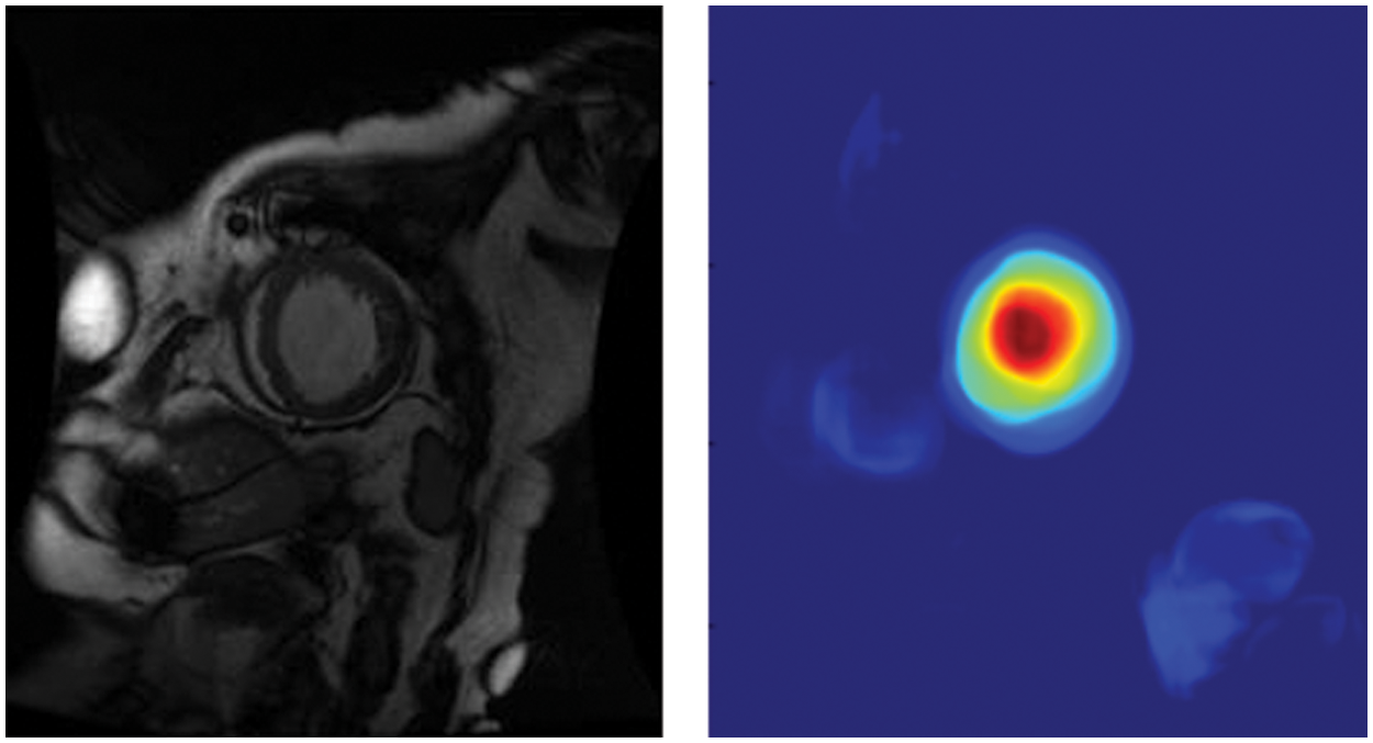
Figure 6: Global average pooling layer visualization

4  Experimental and Evaluation

4.1 Dataset

The Sunnybrook [27,28] data collection contains 45 cine-MRI images of persons with a variety of diseases; healthy people, heart failure with and without infarction, and hypertrophy are some of the terms used. The internal dataset is a sequence of MRI short-axis (SAX) images that have been accurately tagged. The images were originally in DICOM format (256 × 256 grayscale). The label was a tensor with the dimensions of 256 × 256 × 2. These were 2D cine images with about 30 shots spanning the cardiac cycle. Each slice was obtained using a different breath hold. See references [27–29] for a complete list of citations. The training set included 334 images corresponding to 334 different subjects, and the validation set (data not applied for training but used to test the model’s accuracy) included 96 images.

There were four pathological groups in this dataset:

(1)   The patients in the infarction-related heart failure group exhibited a late gadolinium enhancement ejection fraction of less than 40%.

(2)   In the heart failure without infarction group, the ejection fraction was less than 40%, and there was no late gadolinium augmentation.

(3)   The LV hypertrophy group had a normal ejection fraction >55% and a left ventricular mass-to-body-surface-area ratio >83 g/m2.

(4)   The healthy group had an ejection fraction of over 55% and no evidence of hypertrophy.

4.2 Workflow

(1)   Prepare the input data.

(2)   Make a computational graph. Create the neural network graph [27,28] with specific nodes (e.g., inference, loss, and training nodes).

(3)   In a session, loop through the incoming data and inject data into the graph to train the model. Set the number of epochs, batch size, learning rate, and other parameters.

(4)   Examine the model by running inference on previously unknown data (using the same graph from training) and evaluating the model’s accuracy using an appropriate metric.

4.3 Hyperparameter Lookup

Building deep learning models is an iterative, trial-and-error process. Determining the ideal hyperparameter combination is difficult. Experimenting with the input hyperparameters to see how they affect the results can help the designer find the best hyperparameters. Visualization can assist in the speeding up of the process. The following experimental part demonstrates our implementation of this aspect.

In this step, a neural network with the appropriate structure was formed, and an accuracy metric was utilized to illustrate how effectively the network was learning the segmentation task [30]. However, the evaluation accuracy was not as expected; so, the next step was to expand our search of the parameter space. The number of epochs was modified to improve the accuracy score, and a few more parameters were examined. These were as follows:

Learning rate: the initial rate;

Decay rate: the rate at which the initial learning rate deteriorates; for example, 1.0 signifies that there is no degradation, 0.5 indicates halving the per-step rate of decline, and so forth; and

Decay steps: the number of steps that must be completed before the learning rate changes.

After run-back propagation, the learning rate is the frequency with which the weights are adjusted. An excessively high learning rate usually results in changes in the weights due to unusually large values, and the result may bounce around the correct answer rather than converge. The alterations to the weights would be too small under an extremely slow learning rate, and it could take a long time before we arrive at the solution. Using a variable or customizable learning rate is a common approach. A higher learning rate was employed at the start of training; hence, major weight adjustments were performed to reach a nearly workable solution. As the course progressed, we gradually lowered the learning rate until we could focus on a solution. The three characteristics described above aided in controlling the learning rate and the amount and frequency with which it changed [31,32].

4.4 Evaluation Method

The average perpendicular distance (APD) is the distance between an automatically segmented contour and the equivalent manually drawn by an expert; this was calculated and averaged across all contour points in the evaluation. A large number indicates that the two outlines did not match closely [33–36]. The APD is calculated in millimeters using the PixelSpacing DICOM field for spatial resolution.

When we evaluated the accuracy, the evaluation considered exactly what we were computing. The current accuracy statistic merely informed us of how many pixels we were successfully computing. Thus, in Fig. 7, the model assessed the value of a pixel roughly 98% of the time for five epochs. However, it can be seen from the photographs above that the LV region was usually relatively small compared to the overall image size. This resulted in images known as class imbalance [37], in which one class was significantly more likely than the other. In this situation, even if a network were just created to output the result of not a left ventricle for every output pixel, the outcome would still be 95% accurate. Regardless, it would be a waste of time. This demonstrated that excellent segmentation skill did not always indicate high pixel accuracy [38].

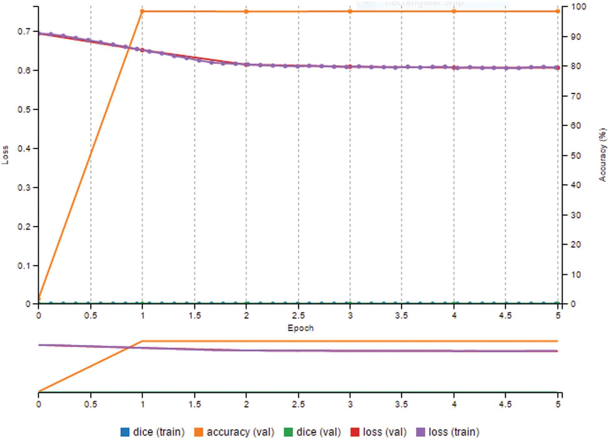
Figure 7: Prediction result is high, but dice metric is zero

The paper calls for an accuracy score that indicates how successfully the CNN segments the left ventricle, regardless of the asymmetry.

The Dice measure, also known as the Sorensen-Dice coefficient, is a metric that can be used to assess how well the network can segment LVs with greater precision. This statistic compares two samples to see how similar they are. In this situation, it was utilized to contrast the two regions of interest, the expertly annotated contour area, and the predicted contour area.

Dicemetric=2AnlAn+Al.(3)

In Fig. 8, the Dice metric can only take a value of zero if there is no intersection between the expected mask and the ground truth. This gives the numerator a value of 0 because 0 divided by anything equals 0. The Dice values have a maximum of 1, indicating that the prediction is 99% accurate. Because they are the same, we have the intersection equal to A or B (the prediction mask or the ground truth). In Fig. 8, when we multiply them by two, we obtain twice the same value divided by two times the same value, yielding a result of 1. This metric will more accurately compute the performance of this model segmenting the left ventricle because the class imbalance [37] problem is negated. Since this study attempted to determine how much area is contained in a particular contour, the pixels can be counted to obtain the area.

Figure 8: Illustration of dice metric

4.5 Experimental Results

Visually monitoring and observing various metrics computed at various epochs, such as loss and accuracy, help to track model progress during the training phase. When the training epoch was raised to 40, there was a noticeable improvement in accuracy. In fact, the 98.3% accuracy was excellent.

A few additional variables were evaluated to improve the score for accuracy. These are as follows:

● Number epochs: 50;

● Decay rate: 0.73;

● Learning rate: 0.02;

● Decay steps: 10,000.

In Fig. 9, this model had a 99.7% accuracy rate and a Dice metric of over 94%.

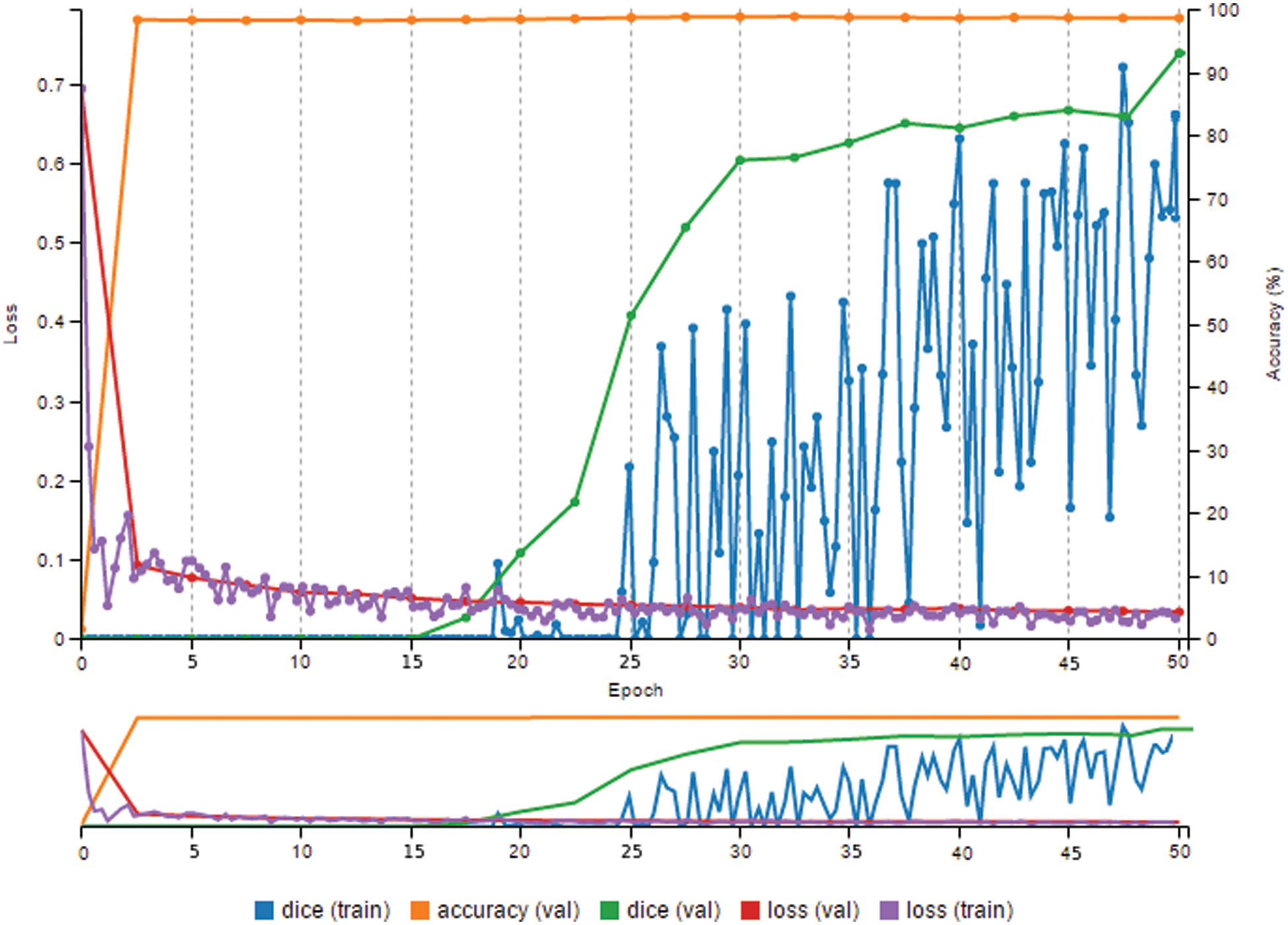
Figure 9: High prediction result and high dice metric

According to Fig. 10, the contour of the prediction by GAP using FCN was smoother, and the predicted results were nearly identical to the initial left ventricular location.

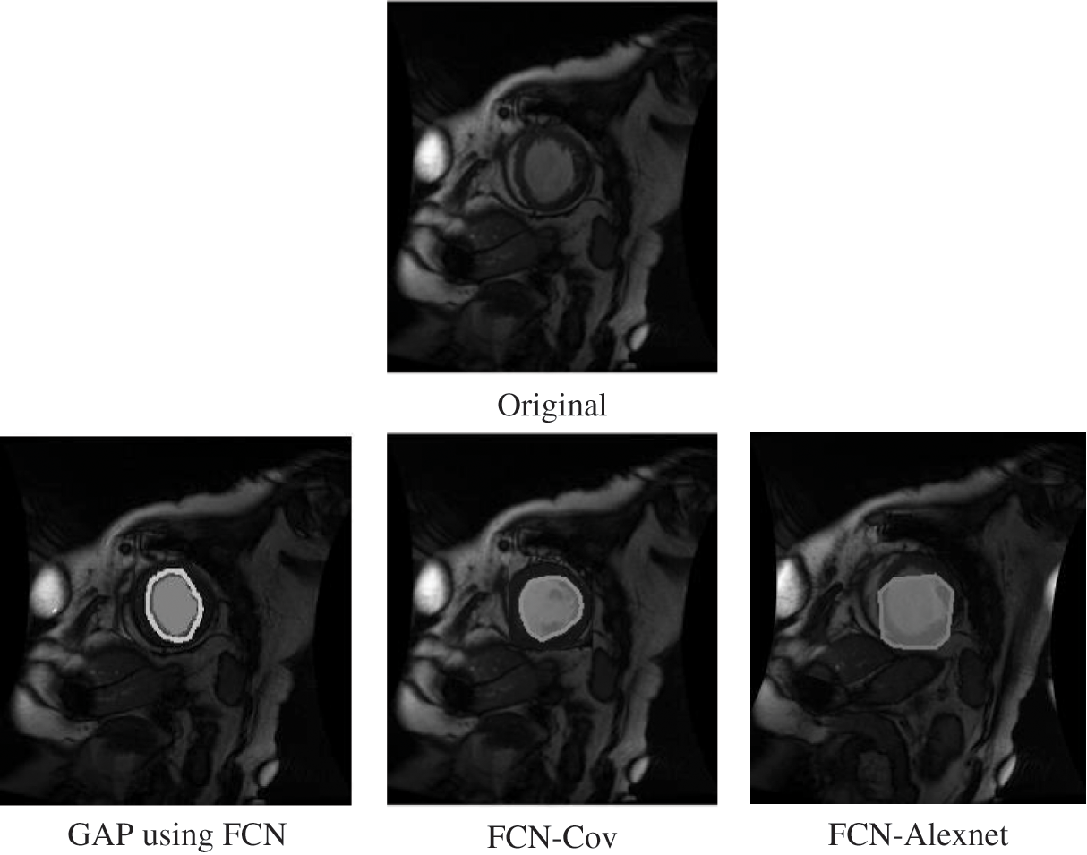
Figure 10: Comparison with other methods

We compared our proposed model to models created by other authors in detail. Table 1 shows that our model is superior to the other models.

5  Discussion and Conclusions

The purpose of this study was to create interpretable CNNs for left ventricle segmentation (MRI) with a balance of accuracy and interpretability based on the interpretability of deep learning approaches. This work differs from standard CNN designs in that explainable methods were supplied for the premodeling analysis and the construction model, the hidden layer was investigated after modeling and the experimental methods, and it provided an assessment method.

In the Sunnybrook Cardiac MR left ventricle dataset, the highest performing algorithms yielded Dice scores of the endocardium between 0.90 and 0.94 [45,46]. We could create a model from scratch that performed as well as the usual ImageNet transfer model. This model was simple and lightweight. If the model was pruned and compressed, it would be suitable to use it to diagnose medical images on mobile devices [49,50].

According to numerous developed learning systems, a system’s interpretability and the model’s performance cannot be optimized simultaneously. Since many of the best-performing models are systems that can be viewed in terms of the inputs and outputs in various visual identification applications, CNNs have recently reached state-of-the-art levels [4–7], including stacked attention and pyramid attention, for example. However, the existing methods often require many labeled images for training. It is quite difficult to obtain many completely annotated photos for image segmentation. For instance, in the ImageNet dataset, there are 14 million images with category labels and 500,000 images with bounding boxes, whereas only 4460 images are pixel-level segmentation results. It is very time-consuming to label the respective pixels in the training images. Some studies used these existing methods to segment MRI images [5] by the transfer learning approach. Nevertheless, the data collection of left ventricle images has only a few pixel-level segmented images; so, the amount of data was small. The extreme right and massive parameters in the model easily cause overfitting. Even though the transfer learning method has achieved high accuracy, it introduces many parameter redundancies to public datasets (e.g., ImageNet, COCONet). It is more difficult to explain convincingly, and many seemingly meaningless model parameters and highly fitting judgment results may be obtained [51,52]. Some research results suggest that attention modules do not provide meaningful explanations and should not be treated as such [13]. Thus, attention approaches cannot provide more trustworthy information. Their use in medical image analysis domains will be limited. Data scientists are more interested in discovering the information the model has gleaned from the images, leading to the ultimate decision.

Developing methods that explain what a model has learned is vital to any comprehensive strategy to maximize clinical acceptance. Nevertheless, most of the AI interpretable research focuses on explaining a black-box model that has already been constructed, i.e., post-modeling explainability [15,16]. Ideally, however, we should avoid the black-box problem from the start by creating a model that can be explained by design. An essential role has been performed by interactive visualization in presenting insights into how deep learning models work [18]. Tensorflow and Pytorch provide effective interactive visualization for comprehending deep learning models; however, most are restricted to simple models and applications. Thus, their applicability is limited.

In this study, based on our upgraded visual deep learning GPU training system, using interpretable CNNs with optimal size and parameters, we presented a novel strategy for autonomously segmenting the left ventricle in a cardiac MRI. It would be ideal for use on smartphones and tablets. DIGITS technologies made deep learning activities easier by showing performance and providing the features of each CNN layer with enhanced real-time visualization. The model’s robustness is better reflected on small datasets, and many existing large models are easily overfitted on small datasets. Some hospitals collect data using their equipment, such as Siemens MR scanners, and create their own private datasets. Modeling on MRI output from the same equipment produces more accurate results, but the sample size is limited due to the small number of patients with left ventricular disease. Our method is ideal for these hospitals to train models on their datasets without requiring a large investment. Our proposed method was feasible and efficient, the Dice metric reached 94.48%, and the accuracy rate reached 99.7%.

Funding Statement: The National Natural Science Foundation of China (62176048) provided funding for this research.

Conflicts of Interest: The authors declare that they have no conflicts of interest to report regarding the present study.

References

1. Samek, W., Montavon, G., Lapuschkin, S., Anders, C. J., Muller, K. R. (2021). Explaining deep neural networks and beyond: A review of methods and applications. Proceedings of IEEE, 109, 247–278. DOI 10.1109/JPROC.2021.3060483. [Google Scholar] [CrossRef]
2. Lee, H., Yune, S., Mansouri, M., Kim, M., Tajmir, S. H. et al. (2019). An explainable deep-learning algorithm for the detection of acute intracranial haemorrhage from small datasets. Nature Biomedical Engineering, 3(3), 173–182. DOI 10.1038/s41551-018-0324-9. [Google Scholar] [CrossRef]
3. Samek, W., Wiegand, T., Müller, K. R. (2017). Explainable artificial intelligence: Understanding, visualizing and interpreting deep learning models. arXiv preprint arXiv:1708.08296. [Google Scholar]
4. Choo, J., Liu, S. (2018). Visual analytics for explainable deep learning. IEEE Computer Graphics and Applications, 38(4), 84–92. DOI 10.1109/MCG.2018.042731661. [Google Scholar] [CrossRef]
5. Samek, W., Montavon, G., Vedaldi, A., Hansen, L. K., Müller, K. R. (2019). Explainable AI: Interpreting, explaining and visualizing deep learning. German: Springer Nature Press. [Google Scholar]
6. Zhang, Q., Wu, Y. N., Zhu, S. C. (2018). Interpretable convolutional neural networks. Proceedings of the 2018 IEEE/CVF Conference on Computer Vision and Pattern Recognition, pp. 8827–8836. Salt Lake City, UT, USA. [Google Scholar]
7. Assaf, R., Schumann, A. (2019). Explainable deep neural networks for multivariate time series predictions. Proceedings of the Twenty-Eighth International Joint Conference on Artificial Intelligence (IJCAI-19), pp. 10–16. Macao, China. [Google Scholar]
8. Kuo, C. C. J., Zhang, M., Li, S., Duan, J., Chen, Y. (2018). Interpretable convolutional neural networks via feedforward design. Proceedings of the 2018 IEEE/CVF Conference on Computer Vision and Pattern Recognition, pp. 18–23. Salt Lake City, UT, USA. [Google Scholar]
9. Ghosal, S., Blystone, D., Singh, A. K., Ganapathy S. B., Singh, A. et al. (2018). An explainable deep machine vision framework for plant stress phenotyping. Proceedings of the National Academy of Sciences, 115(18), 4613–4618. DOI 10.1073/pnas.1716999115. [Google Scholar] [CrossRef]
10. Zheng, Q., Delingette, H., Ayache, N. (2019). Explainable cardiac pathology classification on cine MRI with motion characterization by semi-supervised learning of apparent flow. Medical Image Analysis, 56, 80–95. DOI 10.1016/j.media.2019.06.001. [Google Scholar] [CrossRef]
11. Alarcon, N. (2018). NVIDIA announces the transfer learning toolkit and AI assisted annotation SDK for medical imaging. https://developer.nvidia.com/blog/nvidia-announces-the-transfer-learning-toolkit-and-ai-assisted-annotation-sdk-for-medical-imaging/. [Google Scholar]
12. Raghu, M., Zhang, C., Kleinberg, J., Bengio, S. (2019). Transfusion: Understanding transfer learning for medical imaging. Advances in Neural Information Processing Systems, 32, 3347–3357. [Google Scholar]
13. Jain, S., Wallace, B. C. (2019). Attention is not explanation. arXiv preprint arXiv:1902.10186. [Google Scholar]
14. Wu, B., Fang, Y., Lai, X. (2020). Left ventricle automatic segmentation in cardiac MRI using a combined CNN and U-net approach. Computerized Medical Imaging and Graphics, 82, 101719. DOI 10.1016/j.compmedimag.2020.101719. [Google Scholar] [CrossRef]
15. Sinha, A., Dolz, J. (2020). Multi-scale self-guided attention for medical image segmentation. IEEE Journal of Biomedical and Health Informatics, 25(1), 121–130. DOI 10.1109/JBHI.6221020. [Google Scholar] [CrossRef]
16. Cai, Y., Wang, Y. (2021). Ma-Unet: An improved version of unet based on multi-scale and attention mechanism for medical image segmentation. 2021 Third International Conference on Electronics and Communication, Network and Computer Technology, Harbin, China. [Google Scholar]
17. Brunese, L., Mercaldo, F., Reginelli, A., Santone, A. (2020). Explainable deep learning for pulmonary disease and coronavirus COVID-19 detection from X-rays. Computer Methods and Programs in Biomedicine, 196, 105608. DOI 10.1016/j.cmpb.2020.105608. [Google Scholar] [CrossRef]
18. Vuppala, S. K., Behera, M., Jack, H., Bussa, N. (2020). Explainable deep learning methods for medical imaging applications. 2020 IEEE 5th International Conference on Computing Communication and Automation (ICCCA), pp. 30–31. Greater Noida, UP, India. [Google Scholar]
19. Liu, S., Kailkhura, B., Loveland, D., Han, Y. (2019). Generative counterfactual introspection for explainable deep learning. 2019 IEEE Global Conference on Signal and Information Processing (GlobalSIP), pp. 11–14. Ottawa, BC, Canada. [Google Scholar]
20. Lin, Y. C., Lee, Y. C., Tsai, W. C., Beh, W. K., Wu, A. Y. (2020). Explainable deep neural network for identifying cardiac abnormalities using class activation map. 2020 Computing in Cardiology, pp. 1–4. Rimini, Italy. [Google Scholar]
21. Long, J., Shelhamer, E., Darrell, T. (2015). Fully convolutional networks for semantic segmentation. Proceedings of the IEEE Conference on Computer Vision and Pattern Recognition, pp. 3431–3440. Boston, MA, USA. [Google Scholar]
22. NVIDIA Corporation & Affiliates (2022). DIGITS user guide: NVIDIA deep learning DIGITS. https://docs.nvidia.com/deeplearning/digits/digits-user-guide/index.html. [Google Scholar]
23. Das, A., Rad, P. (2020). Opportunities and challenges in explainable artificial intelligence: A survey. Computing Research Repository. arXiv preprint arXiv:2006.11371. [Google Scholar]
24. Brownlee, J., Imbalanced Classification (2019). A gentle introduction to imbalanced classification. https://machinelearningmastery.com/what-is-imbalanced-classification/. [Google Scholar]
25. NVIDIA (2021). https://developer.nvidia.com/digits. [Google Scholar]
26. MathWorks (2022). Deep learning visualization methods. https://www.mathworks.com/help/deeplearning/ug/deep-learning-visualization-methods.html. [Google Scholar]
27. Sunnybrook Cardiac MR Database (2022). Is made available under the CC0 1.0 universal license described above. http://creativecommons.org/publicdomain/zero/1.0/. [Google Scholar]
28. Radau, P., Lu, Y., Connelly, K., Paul, G., Dick, A. J. et al. (2022). Evaluation framework for algorithms segmenting short axis cardiac MRI. The MIDAS Journal-Cardiac MR Left Ventricle Segmentation Challenge, 2009, 49. http://hdl.handle.net/10380/3070. [Google Scholar]
29. Jonathan, L., Evan, S., Trevor, D. (2018). Fully convolutional networks for semantic segmentation. http://fcn.berkeleyvision.org/. [Google Scholar]
30. Hartnett, K. (2018). To build truly intelligent machines, teach them cause and effect. https://www.quantamagazine.org/to-build-truly-intelligent-machines-teach-them-cause-and-effect-20180515/. [Google Scholar]
31. Pope, P. E., Kolouri, S., Rostami, M., Martin, C. E., Hoffmann, H. (2019). Explainability methods for graph convolutional neural networks. Proceedings of the IEEE/CVF Conference on Computer Vision and Pattern Recognition, pp. 10764–10773. Long Bench, CA, USA. [Google Scholar]
32. Singh, A., Sengupta, S., Lakshminarayanan, V. (2020). Explainable deep learning models in medical image analysis. Journal of Imaging, 6(6), 52. [Google Scholar]
33. Zeiler, M. D., Krishnan, D., Taylor, G. W., Fergus, R. (2010). Deconvolutional networks. Proceedings of the 2010 IEEE Computer Society Conference on Computer Vision and Pattern Recognition, pp. 13–18. San Francisco, CA, USA. [Google Scholar]
34. Alain, G., Bengio, Y. (2017). Understanding intermediate layers using linear classifier probes. https://arxiv.org/abs/1610.01644. [Google Scholar]
35. Pérez-Pelegrí, M., Monmeneu, J. V., López-Lereu, M. P., Pérez-Pelegrí, L., Maceira, A. M. et al. (2021). Automatic left ventricle volume calculation with explainability through a deep learning weak-supervision methodology. Computer Methods and Programs in Biomedicine, 208, 106275. DOI 10.1016/j.cmpb.2021.106275. [Google Scholar] [CrossRef]
36. Bernard, O., Lalande, A., Zotti, C., Cervenansky, F., Yang, X. et al. (2018). Deep learning techniques for automatic MRI cardiac multi-structures segmentation and diagnosis: Is the problem solved? IEEE Transactions on Medical Imaging, 37(11), 2514–2525. [Google Scholar]
37. Ronneberger, O., Fischer, P., Brox, T. (2015). U-Net: Convolutional networks for biomedical image segmentation. International Conference on Medical Image Computing and Computer-Assisted Intervention, pp. 234–241. Munich, German. [Google Scholar]
38. Zhou, Z., Siddiquee, M. M. R., Tajbakhsh, N., Liang, J. (2018). UNet++: A nested U-net architecture for medical image segmentation. Proceedings of the Deep Learning in Medical Image Analysis and Multimodal Learning for Clinical Decision Support, pp. 3–11. Granada, Spain, German: Springer-Verlag Press. [Google Scholar]
39. Schlemper, J., Oktay, O., Schaap, M., Heinrich, M., Kainz, B. et al. (2019). Attention gated networks: Learning to leverage salient regions in medical images. Medical Image Analysis, 53, 197–207. Netherland: ELSEVIER Press. [Google Scholar]
40. Queiros, S., Barbosa, D., Heyde, B., Morais, P., Vilaca, J. L. et al. (2014). Fast automatic myocardial segmentation in 4D cine CMR datasets. Medical Image Analysis, 18, 1115–1131. [Google Scholar]
41. Ngo, T. A., Carneiro, G. (2014). Fully automated non-rigid segmentation with distance regularized level set evolution initialized and constrained by deep-structured inference. Proceedings of the 2014 IEEE Conference on Computer Vision and Pattern Recognition, pp. 23–28. Columbus, OH, USA. [Google Scholar]
42. Jolly, M. P. (2009). Fully automatic left ventricle segmentation in cardiac cine MR images using registration and minimum surfaces. The MIDAS Journal-Cardiac MR Left Ventricle Segmentation Challenge, 4, 59. DOI 10.54294/aidt6e. [Google Scholar] [CrossRef]
43. Liu, H., Hu, H., Xu, X., Song, E. (2012). Automatic left ventricle segmentation in cardiac MRI using topological stable-state thresholding and region restricted dynamic programming. Academic Radiology, 19(6), 723–731. DOI 10.1016/j.acra.2012.02.011. [Google Scholar] [CrossRef]
44. Su, H., Liu, J., Lee, L. C., Venkatesh, S. K., Teo, L. et al. (2011). An image-based comprehensive approach for automatic segmentation of left ventricle from cardiac short axis cine MR images. Journal of Digital Imaging, 24(4), 598–608. DOI 10.1007/s10278-010-9315-4. [Google Scholar] [CrossRef]
45. Wijnh, W. J., Hendriksen, D., Assen, H., Der, G. R. (2009). LV challenge LKEB contribution: Fully automated myocardial contour detection. The MIDAS Journal, 43, 2. [Google Scholar]
46. Liu, J., Deng, F., Yuan, G., Lin, X., Song, H. et al. (2022). An explainable convolutional neural networks for automatic segmentation of the left ventricle in cardiac MRI. Proceedings of the CECNet 2021, pp. 18–21. Beijing, China. [Google Scholar]
47. Marak, L., Cousty, J., Najman, L., Talbot, H. (2009). 4D morphological segmentation and the MICCAI LV-segmentation grand challenge. MIDAS Journal-Cardiac MR Left Ventricle Segmentation Challenge, London, UK. DOI 10.1111/j.1095-8339.2012.01279.x. [Google Scholar] [CrossRef]
48. O’Brien, S., Ghita, O., Whelan, P. F. (2009). Segmenting the left ventricle in 3D using a coupled ASM and a learned non-rigid spatial model, 3D segmentation in the clinic: A grand challenge III [workshop]. The 12th International Conference on Medical Image Computing and Computer Assisted Intervention, pp. 20–24. London, UK. [Google Scholar]
49. Yuan, G., Dong, P., Sun, M., Niu, W., Li, Z. et al. (2021). Work in progress: Mobile or FPGA? A comprehensive evaluation on energy efficiency and a unified optimization framework. Proceedings of the 2021 IEEE 27th Real-Time and Embedded Technology and Applications Symposium (RTAS), pp. 493–496. Nashville, TN, USA. [Google Scholar]
50. Yuan, G., Dong, P., Sun, M., Niu, W., Li, Z. et al. (2022). Mobile or FPGA? A comprehensive evaluation on energy efficiency and a unified optimization framework. 2021 IEEE 27th Real-Time and Embedded Technology and Applications Symposium (RTAS), pp. 493–496. Nashville, TN, USA. [Google Scholar]
51. Liu, J., Yuan, G., Huang, H., Zhang, W., Lin, X. et al. (2022). Brain tumor classification on MRI in light of molecular markers. The 24th International Conference on Artificial Intelligence, The 2022 World Congress in Computer Science, Computer Engineering, & Applied Computing, Las Vegas, USA. [Google Scholar]
52. Liu, J., Deng, F., Yuan, G., Yang, C., Song, H. et al. (2022). An efficient CNN for radiogenomic classification of low-grade gliomas on MRI in a small dataset. Wireless Communications and Mobile Computing, 2022, 8856789. DOI 10.1155/2022/8856789. [Google Scholar] [CrossRef]
Cite This Article
Copyright © 2023 The Author(s). Published by Tech Science Press.
This work is licensed under a Creative Commons Attribution 4.0 International License , which permits unrestricted use, distribution, and reproduction in any medium, provided the original work is properly cited.
Downloads
Citation Tools