
 Submit a Paper
 Propose a Special lssue
 Open Access
ARTICLE
Towards a Unified Single Analysis Framework Embedded with Multiple Spatial and Time Discretized Methods for Linear Structural Dynamics
Department of Mechanical Engineering, University of Minnesota, Twin Cities, Minneapolis, 55455, USA
* Corresponding Author: Kumar K. Tamma. Email:
Computer Modeling in Engineering & Sciences 2023, 135(2), 843-885. https://doi.org/10.32604/cmes.2023.023071
Received 07 April 2022; Accepted 01 July 2022; Issue published 27 October 2022
 View Full Text
 Download PDF
Abstract
We propose a novel computational framework that is capable of employing different time integration algorithms and different space discretized methods such as the Finite Element Method, particle methods, and other spatial methods on a single body sub-divided into multiple subdomains. This is in conjunction with implementing the well known Generalized Single Step Single Solve (GS4) family of algorithms which encompass the entire scope of Linear Multistep algorithms that have been developed over the past 50 years or so and are second order accurate into the Differential Algebraic Equation framework. In the current state of technology, the coupling of altogether different time integration algorithms has been limited to the same family of algorithms such as the Newmark methods and the coupling of different algorithms usually has resulted in reduced accuracy in one or more variables including the Lagrange multiplier. However, the robustness and versatility of the GS4 with its ability to accurately account for the numerical shifts in various time schemes it encompasses, overcomes such barriers and allows a wide variety of arbitrary implicit-implicit, implicit-explicit, and explicit-explicit pairing of the various time schemes while maintaining the second order accuracy in time for not only all primary variables such as displacement, velocity and acceleration but also the Lagrange multipliers used for coupling the subdomains. By selecting an appropriate spatial method and time scheme on the area with localized phenomena contrary to utilizing a single process on the entire body, the proposed work has the potential to better capture the physics of a given simulation. The method is validated by solving 2D problems for the linear second order systems with various combination of spatial methods and time schemes with great flexibility. The accuracy and efficacy of the present work have not yet been seen in the current field, and it has shown significant promise in its capabilities and effectiveness for general linear dynamics through numerical examples.Keywords
As numerical analysis is utilized in the various fields and applications, the desire for analyzing complex problems more efficiently has grown. The Finite Element Method (FEM) is one of the most widely used numerical analysis methods. While it features simplicity and versatility, it is susceptible to numerical errors such as shear locking and complexity in adopting it for large deformation problems and the like.
Concurrently, the strong form based particle methods has been gaining interest in the field of numerical simulations as the particle methods have the capability and flexibility for handling large distortion, crack propagation and free surface detecting, etc. Some of the notable strong form particle methods, Smoothed Particle Hydrodynamics (SPH) [1–4] and Moving Particle Semi-implicit Method (MPS) [5,6], have been used to solve partial differential equations. Later, Silling et al. proposed a nonlocal extension of classical continuum mechanics called peridynamics (PD) [7,8], which represents spatial derivatives of field quantities in terms of internal interactions between points/particles via integrals involving differences. The peridynamics model shows a comprehensive ability to solve linear and nonlinear second order system problems and simulate structural dynamics and molecular dynamics as well as multi-scale problems [9]. More recently, a mixed form representation of the strong form particle method, where multiple primary variables are solved at once, is presented in [10]. Other related works appear in references [11–14].
As problems become more complex, controlling the spatial discretization locally is a desirable feature. While an area where fast dynamics are presented is discretized with high spatial resolutions, a coarser mesh may be sufficient in the majority of the structure. In addition, the selection of spatial methods in different parts of a body can also be an effective strategy such as by utilizing the FEM for the majority of a body, and applying particle based methods only on an area where localized phenomena such as crack or fracture may occur.
One of the ways to locally control spatial discretization is dividing a body into regions of subdomains in which different methods can be applied in each subdomain. The challenge in using subdomains is handling the interface condition between the subdomains, and over the years, numerous coupling methods have been developed. Interface coupling is largely divided into two categories: overlapping and non-overlapping domain coupling. In the case of the overlapping domain decomposition, a portion of the subdomains are overlapped and the shape function similar to the framework of the FEM is used to constrain the common Degrees of Freedom (DOFs). However, the large difference in each of the subdomain’s stiffness may lead to the global stiffness matrix to be ill-conditioned, as noted by Orsini et al. in [15]. Moreover, Metsis et al. [16] implied that the weak form based domain decomposition methods may be more prone to this issue due to the implementation of the Gaussian integral.
On the other hand, the non-overlapping technique is more straight forward where the subdomains are only connected by an edge or a surface in 2D or 3D, respectably, and are constrained by the Lagrange multiplier at the interface. At the interface, usually the nodes/particles are overlapped; however, Park et al. [17] and Brezzi et al. [18] introduced an approach where the subdomains are not directly interacting but through an intermediate interface. This approach allows more flexibility in meshing as one-to-one matching of the nodes is not required.
Implementing the different spatial discretization methods for localized phenomena has been a study which has been explored for many years. The coupling of the FEM with molecular dynamics via a bridging domain which enforces compatibility by utilizing the Lagrange multiplier is proposed by Xiao et al. [19]. Alternately, the Discrete Element Method (DEM) [20] is a widely used mesh-free method in the rock engineering simulation field and various FEM-DEM coupling methods have been developed [21,22]. Utilizing the peridynamics method for localized phenomena such as crack propagation is also a topic with extensive studies including coupling the FEM and the PD [23–25]. In this work, one to one node/particle matching is used to simply demonstrate the concept of coupling different spatial methods and different time integration schemes unlike state of art which is limited to just the spatial methods. We couple the FEM and particle methods with different time schemes for each subdomain and such features are not feasible in the state of art.
There also has been high interest in coupling subdomains for transient analysis. Gravouil et al. presented the GC method in [26], employing different time increments in subdomains using the limited Newmark family of algorithms. However, it was later discovered that artificial numerical dissipation arises at the interface resulting in the loss of energy and loss of second order accuracy in the GC method.
Similarly, Pegon extended the GC method and proposed the PM method which employs an inter-field parallel solution procedure to couple different subdomains [27,28]. Prakash et al. [29] developed the PH method in order to alleviate the GC method’s energy issue by solving the interface at a large time scale. The drawback of the PH method was described by Karimi et al. who stated in [30], that the PH method can only apply to two subdomains. Karimi et al. [30] developed the subdomain DAE framework for the Newmark family of algorithms. A noteworthy aspect of this work is that the constrained continuous system in time is in fact a system of differential algebraic equations rather than ordinary differential equations in time which most coupling methods have been based upon. Nakshatrala et al. later applied the DAE approach to the Finite Element Tearing and Interconneting (FETI) method based domain decomposition to solve time dependent first order systems with the fourth order Nakshatrala et al. [31]. More recently, Shimada [32] integrated the Generalized Single Step Single Solve (GS4) family of algorithms with the subdomain DAE framework using the FEM. And, Maxam et al. [33] proposed an unified approach of the DAE-GS4 framework on thermoelastic problems using the FEM. There exists interest in coupling different subdomains for transient analysis. However, the current algorithm technology is very limited and does not permit features to interface a wide variety of time algorithms and spatial methods. And, this is the focus of the advances and contributions of this paper.
In this work, the subdomain DAE framework is particularly advanced to the Generalized Single Step Single Solve (GSSSS or GS4) framework and family of algorithms developed by Tamma et al. [34–37]. The versatility of the GSSSS family of algorithms in the treatment of numerical dissipation, overshoot and ease of adapting to explicit methods, proves extremely useful to the subdomain framework. In addition, the coupling of the FEM based on the weak form, and the generalized particle method (GPS) based on the strong form is also presented in this work to demonstrate integrating altogether different spatial methods as well. The coupling of different spatial and time discretization methods may lead to more accurate computation as it allows the selection of the appropriate method for a specific situation. The novel GS4 framework and its family of algorithms is a general purpose structure. It encompasses the entire class of Linear Multistep (LMS) methods including those that have been developed over the past 50 years or so and in addition, also includes new and advanced optimal designs of algorithms, in 1st/2nd order systems that are second order time accurate and used for commercial software to enable practical real word applications to be conducted. In addition, under one umbrella, the frameworks inherit and have new and optimal algorithms and designs in addition to existing methods such as Crank-Nicolson, Gear’s BDF, etc. for first order systems; and new and optimal choices in second order systems as well in contrast to existing ones such as the Newmark family, HHT, WBZ and the like. A particularly unique feature is that the framework permits interfacing a wide variety of implicit-implicit, implicit-explicit, and explicit-explicit algorithm designs in a single analysis unlike the existing methods which are limited and not capable of doing so; in particular coupling of different implicit-implicit algorithms with/without controllable numerical dissipation which is not feasible in the current state-of-the-art. This is a significant breakthrough and is capitalized herein. The generality, flexibility and robustness of the present computational framework which embraces subdomain and time integration algorithms and differing spatial methods fused into one is not possible with today’s traditional methods and technology that shows limitations such as reduced order accuracy, consistency problems and the like in various field variables such as displacement, velocity, acceleration and Lagrange multiplier. The present developments provide a wide variety of choices to the analyst. In this work, we consistently preserve and maintain second order time accuracy in all variables such as displacement, velocity and acceleration including the Lagrange multipliers. In this paper, the FEM and GPS are first reviewed to explain the basics in integrating different spatial methods as well as different time integration methods in a single analysis. Then in the following section, the incorporation of the GS4 family of algorithms with the DAE framework is investigated and validated through various numerical examples.
A brief overview of the finite element method is reviewed in this section for better understanding of the various numerical examples and its methodology that are presented in a later section. In addition, the objective is to get clarity of the computations involved in the calculations of the FEM integrals and particle method integrals.
2.1 Finite Element Approximations
In the finite element method, a body of domain
where
where
Quadrilateral elements with two Gauss points in each x and y direction will be used throughout in the numerical example section.
2.2 Weak Form Formulation for FEM
The equilibrium equation expressed in terms of the displacement can be written as (shown for 1D as a simple illustration)
Next we introduce an arbitrary function w(x) that is defined in the domain
Then we integrate over the domain to obtain an integral form that is set to zero.
The stress term is then integrated by parts as
where
Introduce the constitutive equation to obtain governing equation based on displacement, and we get
It is worth noting that we removed
The resulting weak formulation in space is given as
and limiting the trial and test spaces to high fidelity finite element spaces, we get
Setting
The above equation is valid for any
leading to
3.1 Gradient and Divergence of Classical Physical Field
A physical field can be thought of as the assignment of a physical quantity at each point in space and time. Consider a domain in Euclidean space,
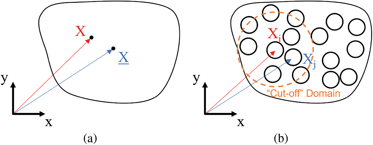
Figure 1: (a) Continuous domain with position vector X and X, (b) Discretized domain with position vectors Xi and Xj
The weighted residual method has been widely used in solving different kinds of ordinary/partial differential equations, in particular, using the Galerkin method, which is the fundamental theory of the finite element method. In this work, we exploit the weighted residual method directly to the Taylor series expansion, such that a generalized approach of developing particle based methods can be explored.
In mathematics, the Taylor series expansion is a representation of a function as an infinite sum of terms that are calculated from the values of the function’s derivatives at a single point. The generalized Taylor series of a general physical quantity
where
Omitting the higher order terms from Eq. (19), we have the first order Taylor series approximation
where
According to the standard weighted residual method, we introduce a weight function, C1, and minimize the residual. Eq. (21) is multiplied by the weight function C and integrated over the domain
It is worth noting that the domain is the cut-off influence domain of the position X, and the residual is a local value. The weight function C provides a wide scope of approximations for constructing the derivative definitions used in various particle-based methods and new approach of particle methods as well.
Gradient Recall the residual R in Eq. (21) and the weighted residual, RC, with respect to a vector property
where C is a vector with the size of geometric dimension of a problem; for example, C is a two by one vector in 2D problems. We postulate that Eq. (23) is the exact relationship between the point X and one of its neighboring point
By treating
Hence, the gradient of a vector can be obtained as
The proposed gradient operator has the ability to recover the ′∇′ in the Moving Particle Semi-implicit (MPS) method, the deformation gradient in the state-based peridynamics as well as in the corrected Smoothed Particle Hydrodynamics (SPH) method, by selecting the appropriate corresponding C.
Remark 3.1. By selecting the arbitrary
Let
Discretizing into particles, and applying
Thus, Eq. (27) can be written as
Gradient Operator:
Introducing the weighting function
It is worth noting that for a general particle within a uniformly distributed system, the weighted average matrix
where
Divergence By representing the divergence model as gradient operator, ∇, dot product with a physical quantity,
The discretized formulations is listed as following
Laplacian The definition of the Laplacian can be written as
In order to obtain the Laplacian relationship between the center point X and its neighboring point
However, the rank of matrix
Therefore, an alternative gradient of a vector is given by taking advantage of the average property, Eq. (37).
Consequently, the Laplacian can be obtained via combining Gauss’s Theorem and the gradient formulations.
where
Therefore, the Laplacian of
Hence the following Laplacian formulations can be obtained as
The discretized formulations is listed as following:
3.2 Stiffness Matrix for Particle Method
We will explore how the stiffness matrix is formed in 2D using the GPS method. We start with the same governing equation and constitutive law,
where D is elastic matrix as following
The first step to get the stiffness matrix is to describe ∇u with the gradient operator from the GPS method as described in Eq. (32).
where [A] is a two by two matrix that is computed first. The summation is applied for every particle within particle i’s influence circle. But for simplicity, we will consider there are two particles for the system, particles 1 and 2. The Eq. (47) will be written as following for particle 1,
Thus,
Next, we need to convert the 2 by 2 matrix on the left hand side of Eq. (50) to a 4 by 1 vector form.
We can also get the engineering strain as follows:
Eq. (52) can be simply written as
Stress
It is worth noting that [D][∇][u] includes all the components in the particle i’s influence domain.
where
Next, we will show how to construct the divergence operator into a matrix form similar to how the gradient operator matrix was formed as shown above.
where
or for the engineering stress,
Thus, we can get the stiffness matrix for the particle 1, by combining Eqs. (55) and (60),
This process is repeated for each particle in the system. After generating
4 Equations of Motion for a System of Multiple Subdomains
Differential Algebraic Equations (DAE) are differential equations with algebraic constraints. Consider the equation of motion of a body that is subject to constraints g(u) = 0. The action integral is given as
and we can take the variation of the action integral,
where G(u) = ∂g(u)/∂u. For the standard DAE equations of second order transient systems, the above equation can be written as
where,
Now, consider a domain of interest
where
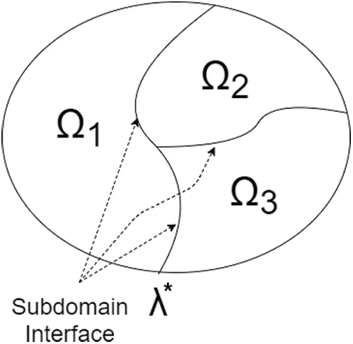
Figure 2: A domain Ω divided into three subdomains with non-overlapping interface
The matrix
4.1 DAE Framework with GS4 Family of Algorithms for a System with Multiple Subdomains and Multiple Time Step Sizes
Let
where n denotes the system time step, and m represents subdomain time step. The visual representation of time subcylcing is shown in Fig. 3.
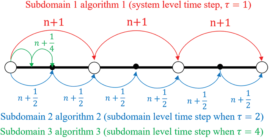
Figure 3: Time step subcycling for different subdomains
Now applying the GS4 family of algorithms, the equation of motion of each subdomain can be written as following:
where
It is worth noting that the Lagrange multipliers are approximated in the system time level rather than in the subdomain time level. This factor suggests that the solution must be in the system time level even though the displacement, velocity, and acceleration are approximated in the subdomain time step.
The updates of each of the unknown variables with the GS4 framework of algorithms are
In linear dynamical systems, Eq. (67) may be written as
where
A set of all kinematic unknowns for
Eq. (71a) can then be discretized and written as follows:
where
with
and
where O represent zero-matrix,
The constraint equation at the velocity level, i.e., Eq. (71b), can be written in the form
where
and
with
Eq. (82) shows the velocity constraint. The size of
The equation of motion for the entire system for a system time step level can be represented in a simple matrix form as following:
where
in which
in which
and
in which
The computation flowchart for the GS4-II DAE framework for the subdomain method employing different spatial methods, algorithms, and time steps is shown below in Fig. 4 which here which provides a wide variety of algorithms and choices as options to the analyst.
for dom := 1 to Ndom do
Calculate M, C, K using corresponding method for the domain
Calculate Li, and Ri using Eqs. (74) and (75a)
Calculate Ĝi using Eq. (82)
for τ := 1 to n do
Assemble Ai using Eq. (85)
Assemble Bi using Eq. (87)
end for
end for
Assemble
Assemble
Transpose
for (t := 1 to Timesteps) do
for dom := 1 to Ndom do
Calculate Fi using Eq. (89)
end for
Assemble
Assemble ^Rglob and Ĵglob from Eq. (83)
Solve (ĴglobXn+1 = ^Rglob)
end for
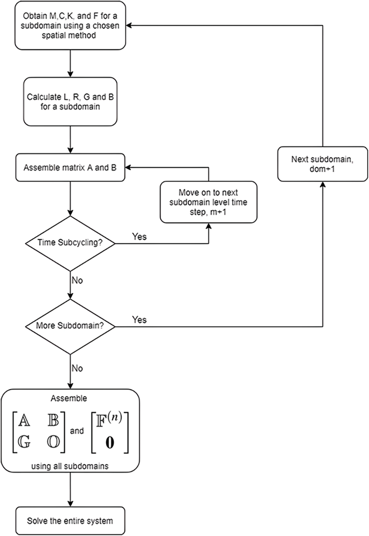
Figure 4: Flowchart for constructing DAE second order system
4.3 Subdomain Coupling Condition and Time Level Consistency for Second Order Systems
The second order time accuracy of all the primary variables and the Lagrange multipliers can be achieved for interfacing different subdomains (this is in general not plausible with traditional methods) if
where
The GS4-II algorithms are written in the form of U0(
With the
For the U0 family of GS4-II algorithms, the
5.1 2D Wave Propagation Problem
Fig. 5 shows the 2D geometry of a wave propagation problem. It is a rectangular bar of 10 m by 1 m with 1 m thickness, which is fixed on the left side wall as boundary condition. The semidiscrete equation of motion for the system is given as
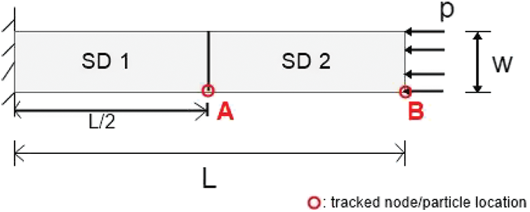
Figure 5: Diagram of structure for wave propagation problem
The bar is compressed from the right side with p, the distributed load, of 10,000 N/m. This material has 72 GPa for Young’s modulus, 0.3 for Poisson’s ratio, and
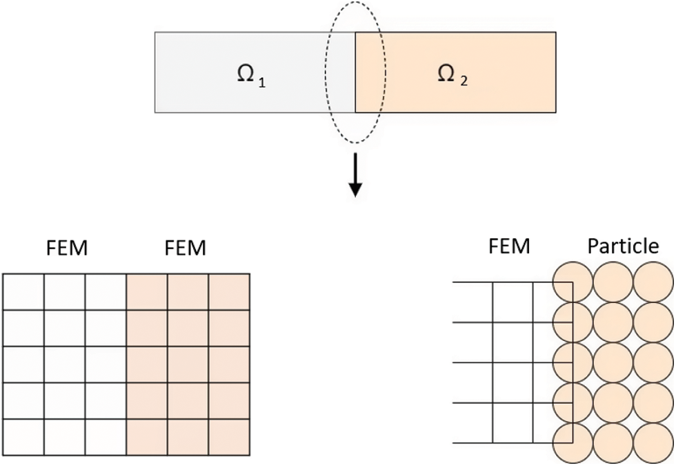
Figure 6: FEM+FEM and FEM+GPS interface
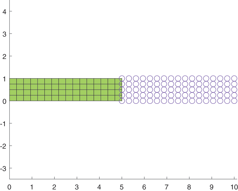
Figure 7: FEM+GPS two domain mesh of the structure
Fig. 8 compares the three different cases of coupling different methods: FEM+FEM, GPS+GPS, and FEM+GPS; and shows the time history of the displacement, velocity, and acceleration at A in subdomain 1 and at point B in subdomain 2. It is clear that coupling the same methods or coupling different methods, be it weak form or strong form methods together, produce a comparable result with the result from commercial software such as ABAQUS.
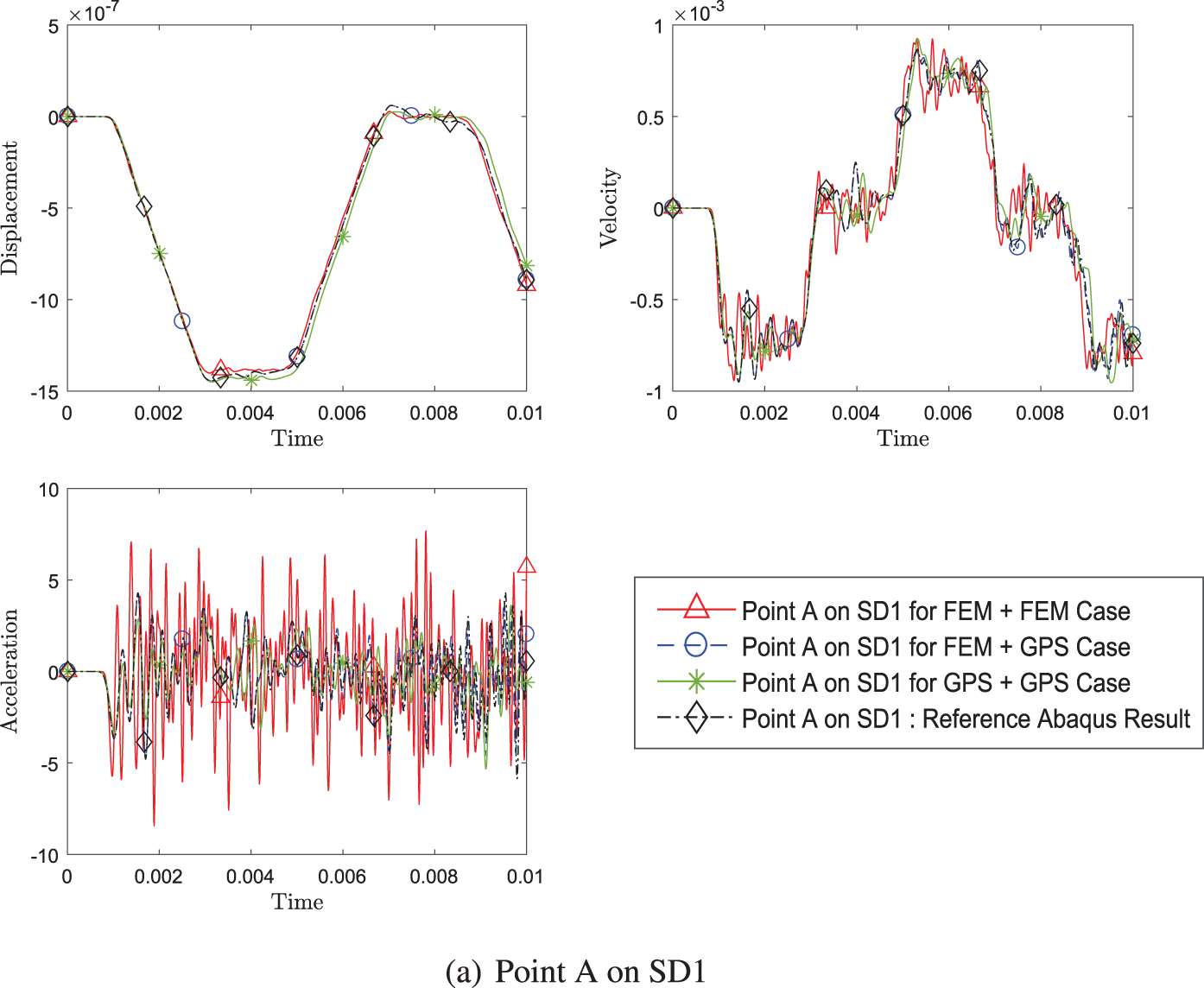
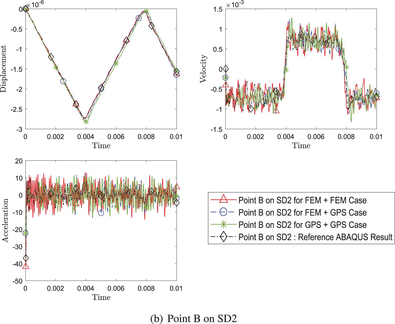
Figure 8: Comparison of transient response of displacement, velocity and acceleration (a) at point A on SD1 and (b) at point B on SD2, between three cases of different pairing of methods (Case 1: FEM+FEM, Case 2: FEM+GPS, Case 3: GPS+GPS) while using explicit version (with η3 = 0) of GS4-II U0(1, 1, 0) algorithm for subomain 1 and explicit version (with η3 = 0) of U0(0, 0, 0) algorithm for subdomain 2 with constant Δt in each case
Fig. 9 shows the result for coupling explicit version and implicit version of the schemes. The evaluated coupling cases are explicit and explicit case, explicit and implicit case, and implicit and explicit case where the first condition refers to the time scheme algorithm for subdomain 1 and the latter for subdomain 2. This figure not only suggests that explicit and implicit time algorithms can be coupled together, it also shows that coupling is not limited to just Newmark family of algorithms as this example couples U0(1, 1, 0) (equivalent to Newmark, central difference for explicit, and average acceleration for implicit) and U0(0, 0, 0) (equivalent to WBZ).
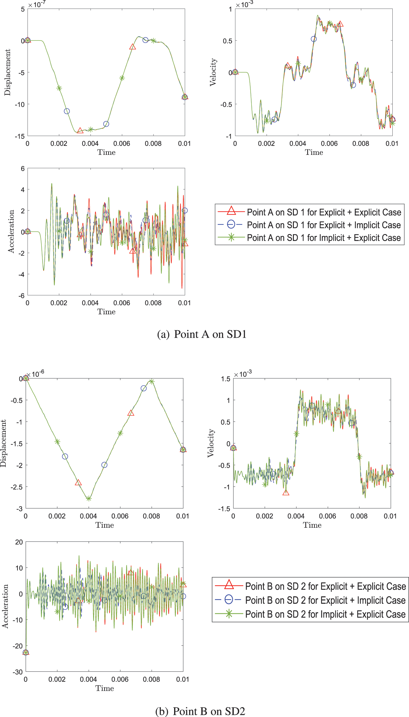
Figure 9: Comparison of transient response of displacement, velocity and acceleration (a) at point A on SD1 and (b) at point B between different pairing of explicit (with η3 = 0) and implicit version (with η3 = 1) of GS4-II (Case 1: explicit+explicit, Case 2: explicit+implicit, Case 3: implicit+explicit) while using FEM with GS4-II U0(1, 1, 0) algorithm for subomain 1 and GPS with U0(0, 0, 0) algorithm for subdomain 2 at constant Δt in each case
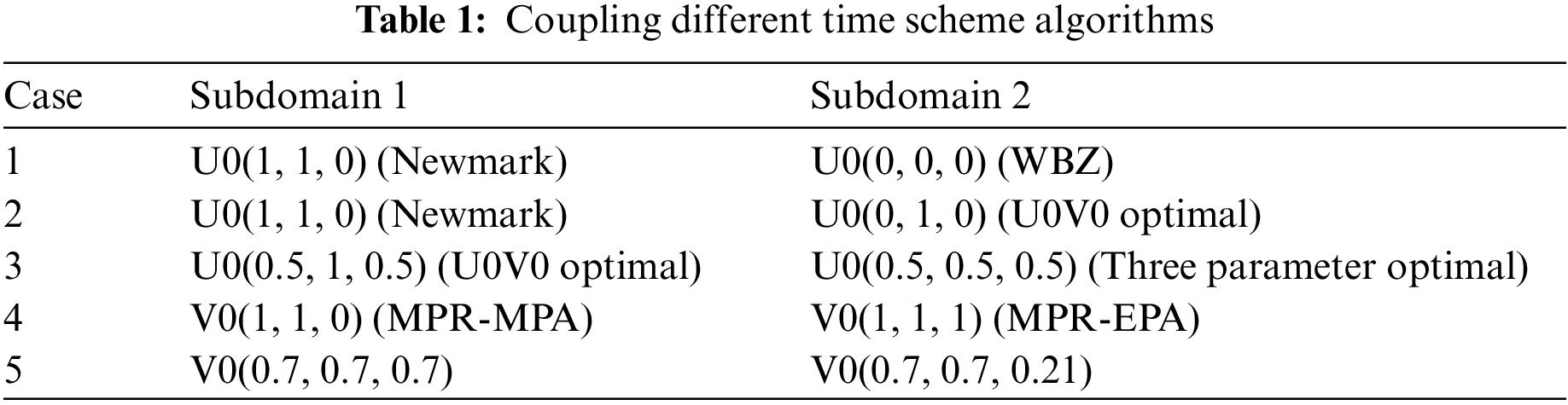
To further present evidence of coupling various time scheme algorithms, five different cases listed in Table 1, are evaluated and illustrated in Fig. 10. The time scheme algorithms are selected such that a combination has identical
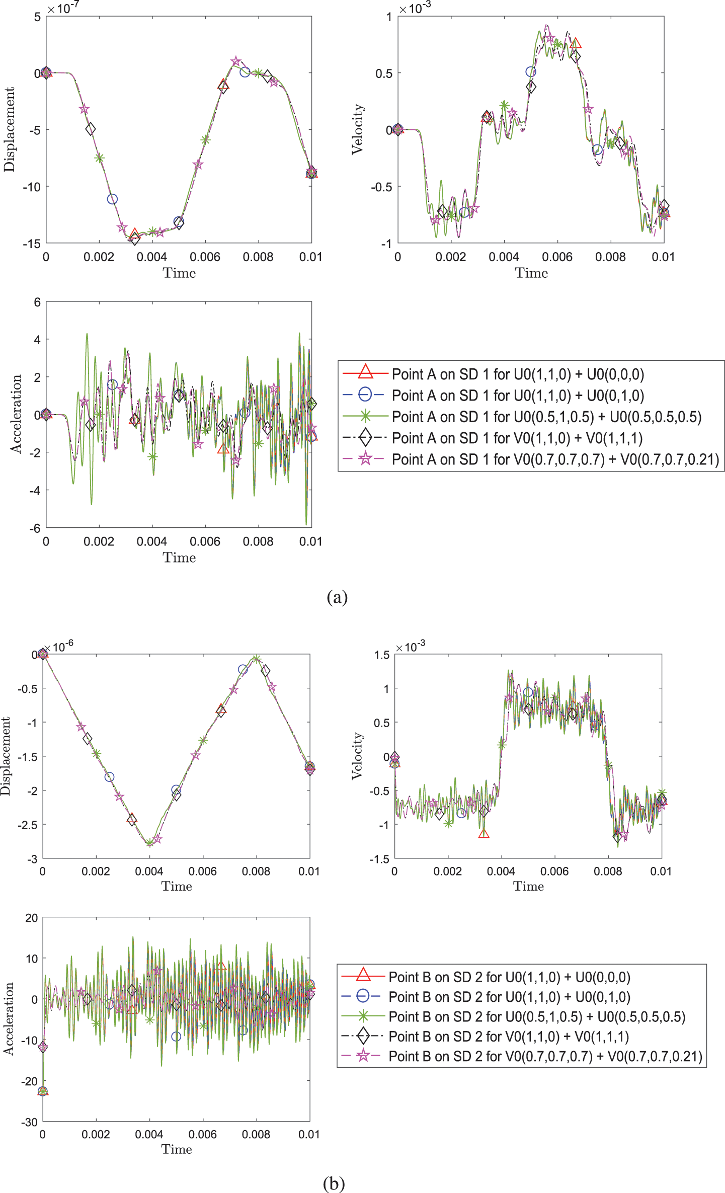
Figure 10: Comparison of transient response of displacement, velocity and acceleration (a) at point A on SD1 and (b) at point B between different pairing of explicit version (with η3 = 0) of GS4-II algorithms listed in Table 1, while using FEM for subdomain 1 and GPS for subdomain 2 at constant Δt in each case
Lastly, the subcycling cases are also evaluated in Fig. 11. A case where subdomain 2 has double the time steps than subdomain 1 (time increment interval in subdomain 2 is half of that of subdomain 1) is compared with the no subcycling case and the results are very close.
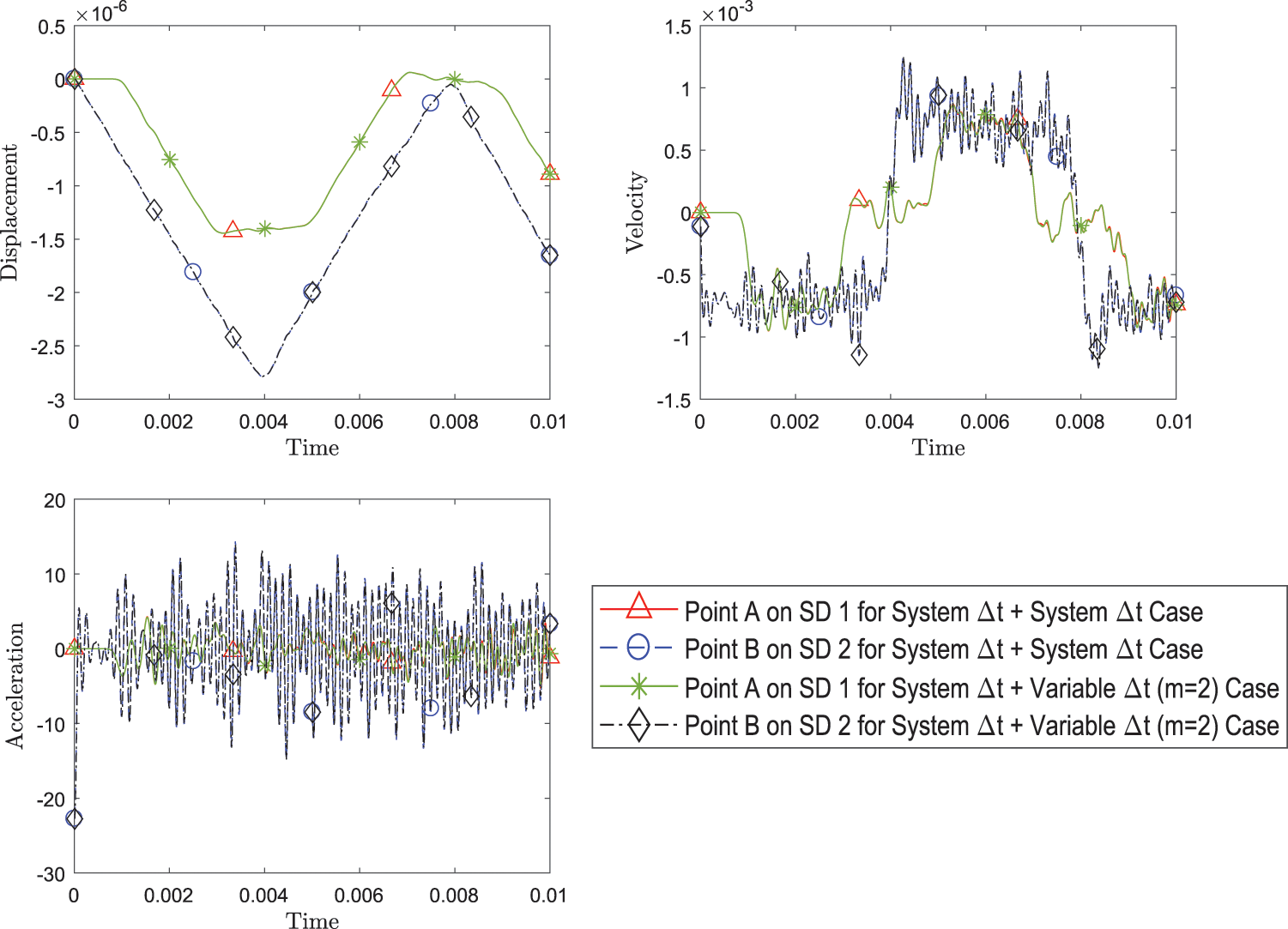
Figure 11: Comparison of transient response of displacement, velocity and acceleration at both point A and point B between simulation with system Δt for both subdomains and with variable Δt = 1/2 system Δt for subdomain 2 while using FEM with explicit version (with η3 = 0) of GS4-II U0(1, 1, 0) algorithm for subdomain 1 and GPS with explicit version (with η3 = 0) U0(0, 0, 0) algorithm for subdomain 2
Fig. 12 demonstrates second order time accuracy in displacement, velocity, acceleration and the constraint variable
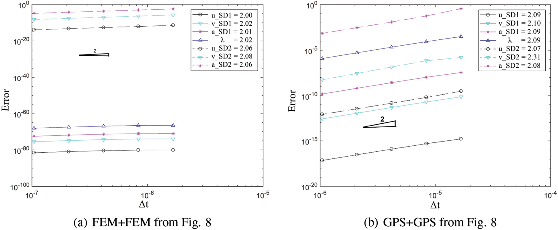
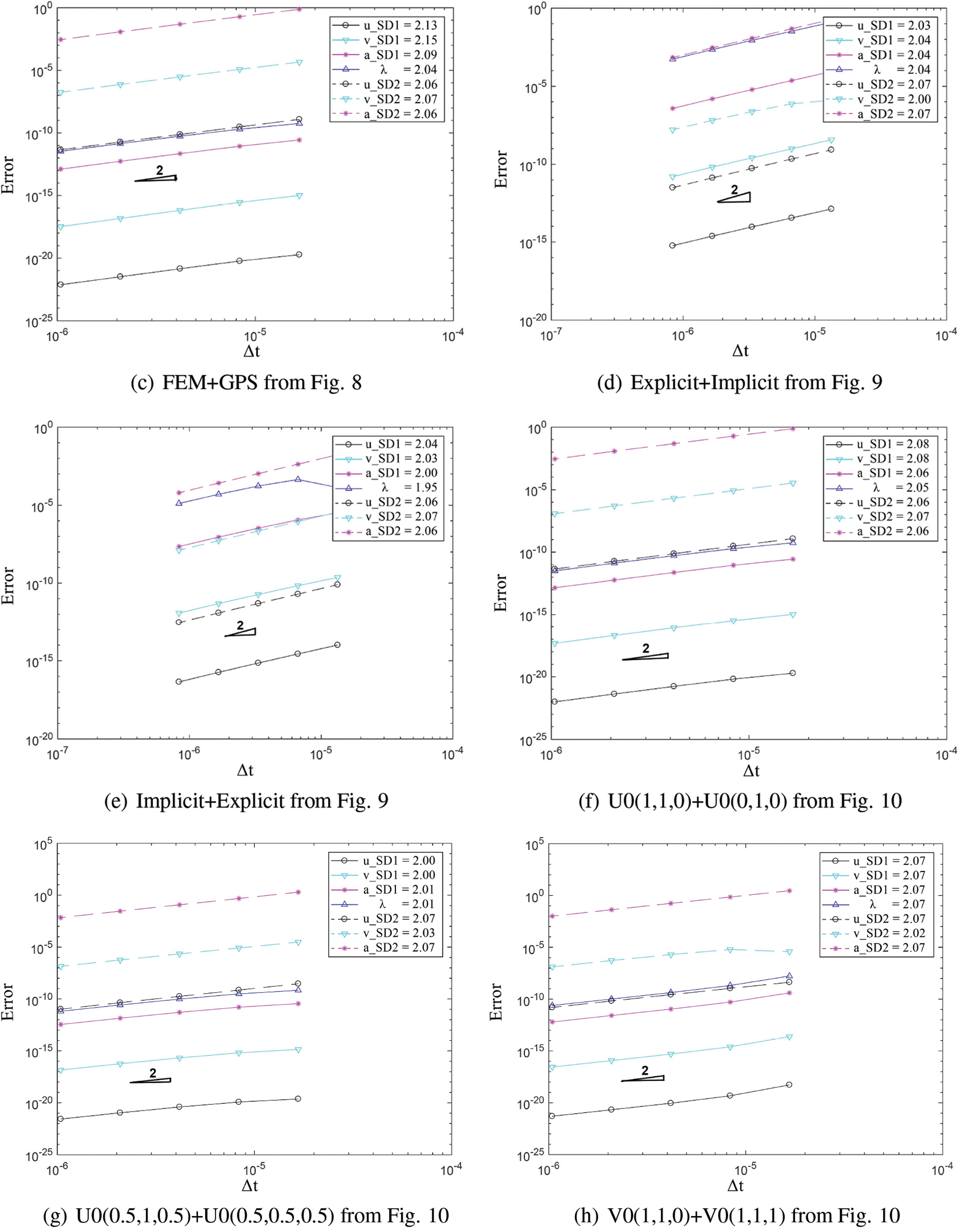
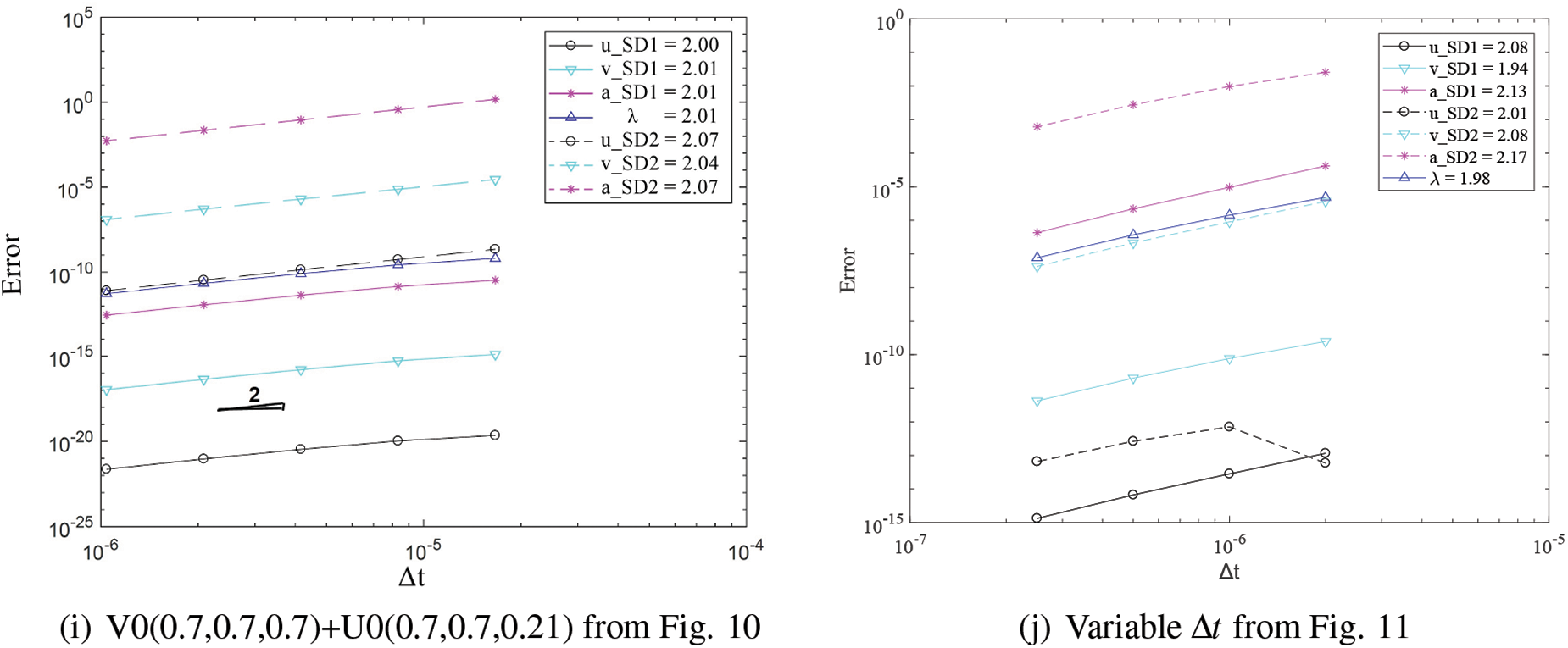
Figure 12: Convergence order for the solution with respect to the system time step for domain 1 and 2 in different cases: (a) FEM with explicit version of GS4-II U0(1, 1, 0) and FEM with U0(0, 0, 0), (b) GPS with explicit version of GS4-II U0(1, 1, 0) and GPS with U0(0, 0, 0), (c) FEM with explicit version of GS4-II U0(1, 1, 0) and GPS with U0(0, 0, 0) algorithm, (d) FEM with explicit version of GS4-II U0(1, 1, 0) and GPS with implicit version U0(0, 0, 0), (e) FEM with implicit version of GS4-II U0(1, 1, 0) and GPS with explicit version U0(0, 0, 0), (f) FEM with explicit version of GS4-II U0(1, 1, 0) and FEM with implicit version U0(0, 1, 0), (g) FEM with explicit version of GS4-II U0(0.5, 1, 0.5) and GPS with U0(0.5, 0.5, 0.5), (h) FEM with explicit version of GS4-II V0(1, 1, 0) and GPS with V0(1, 1, 1), (i) FEM with explicit version of GS4-II V0(0.7, 0.7, 0.7) and GPS with V0(0.7, 0.7, 0.21), (j) variable Δt = 1/2 system Δt for subdomain 2 while using FEM with explicit version (with η3 = 0) of GS4-II U0(1, 1, 0) algorithm for subdomain 1 and GPS with explicit version (with η3 = 0) U0(0, 0, 0) algorithm for subdomain 2
A beam with the same geometry as the one in the wave propagation problem is used to illustrate the application of the multi-domain method in a plane stress dynamic problem. A cantilever beam of 10 m by 1 m with 1 m thickness is fixed on the left side and is experiencing downward traction, p, of 100,000 N/m as shown in Fig. 13. The density,
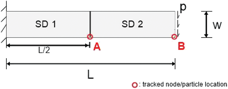
Figure 13: Diagram of structure for bending problem
The system
Similar to the previous problem, a different combination of methods are compared in Fig. 14. It is apparent that the different methods can be coupled regardless of whether one is weak form or strong form.
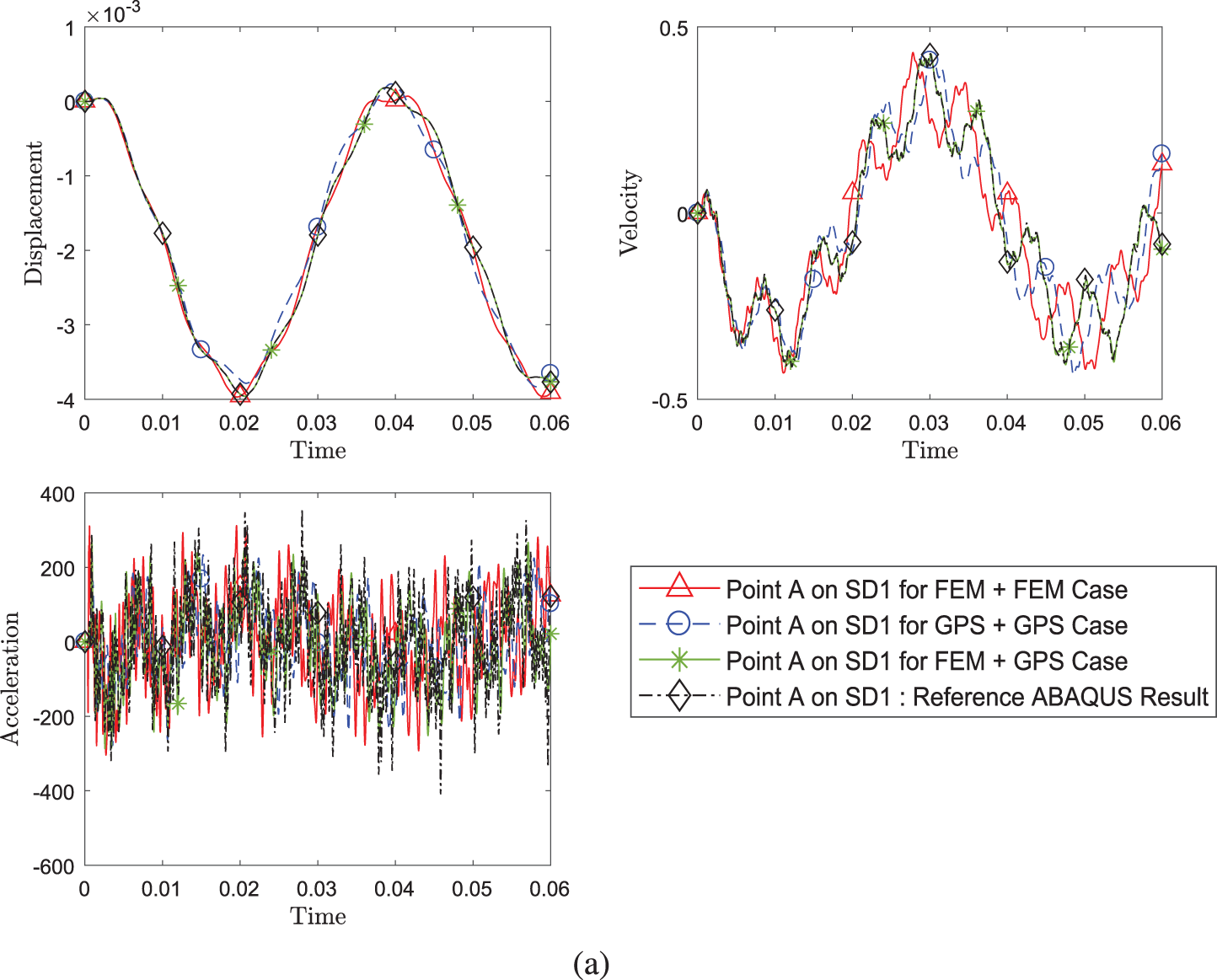
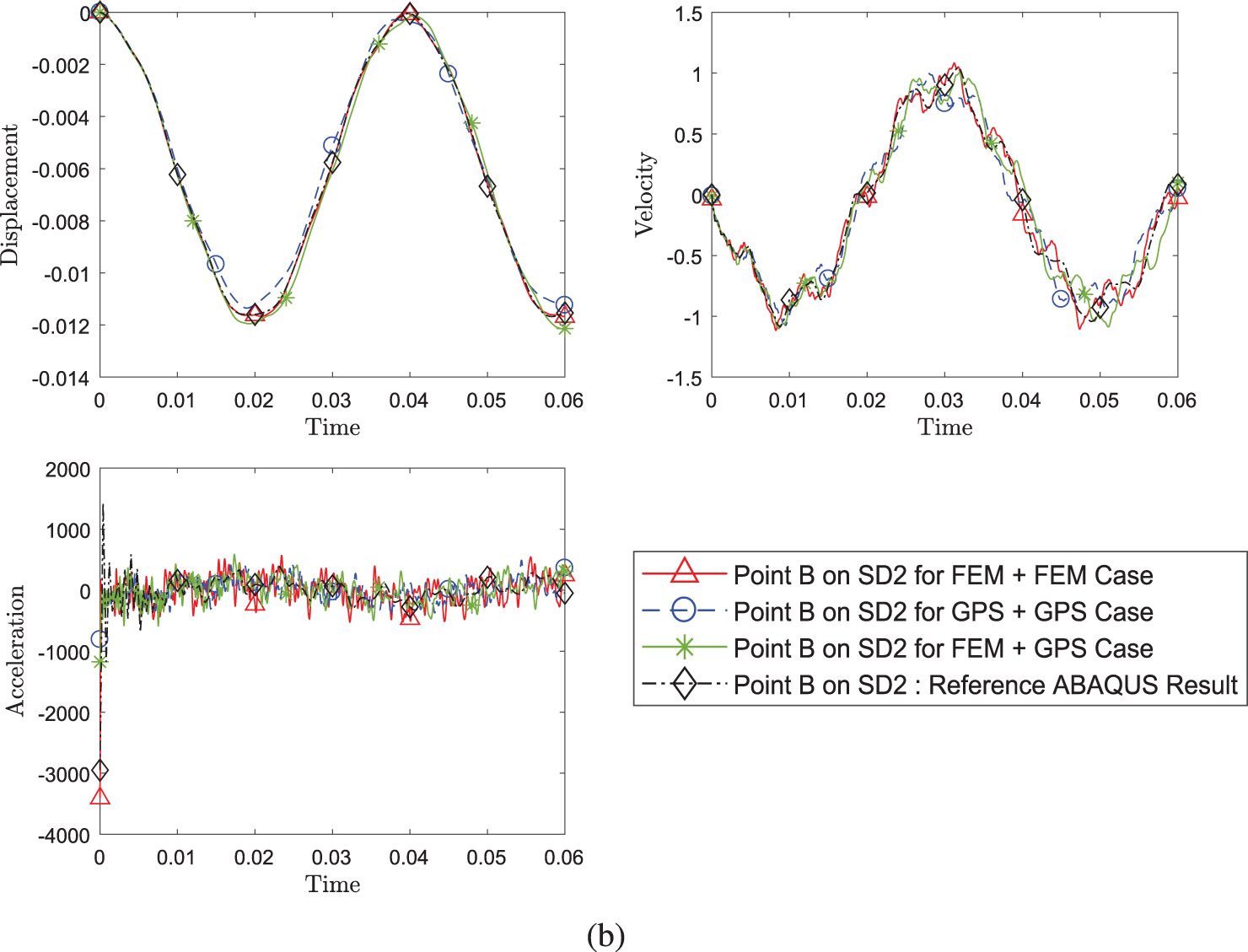
Figure 14: Comparison of transient response of displacement, velocity and acceleration (a) at point A on SD1 and (b) at point B between different pairing of methods (Case 1: FEM+FEM, Case 2: FEM+GPS, Case 3: GPS+GPS) while using implicit version (with η3 = 1) of GS4-II U0(1, 1, 0) algorithm for subdomain 1 and implicit version of U0(0, 0, 0) algorithm for subdomain 2 with constant Δt in each case
Fig. 15 shows results for coupling the explicit version and implicit version of the time scheme algorithms. The evaluated coupling cases this time are the implicit and implicit case, explicit and implicit case, and implicit and explicit case. The response results for the different cases align closely. The same five cases of time scheme algorithm combinations used in the previous example are evaluated and illustrated in Fig. 16. And the results for all cases match. The subcycling case with one domain having half the
Figure 15: Comparison of transient response of displacement, velocity and acceleration (a) at point A on SD1 and (b) at point B between different pairing of explicit (with η3 = 0) and implicit version (with η3 = 1) of GS4-II (Case 1: implicit+implicit, Case 2: explicit+implicit, Case 3: implicit+implicit) while using FEM with GS4-II U0(1, 1, 0) algorithm for subdomain 1 and GPS with U0(0, 0, 0) algorithm for subdomain 2 at constant Δt in each case
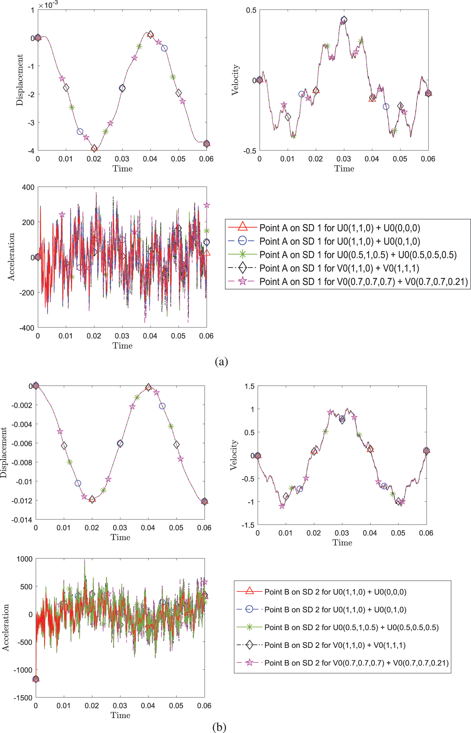
Figure 16: Comparison of transient response of displacement, velocity and acceleration (a) at point A on SD1 and (b) at point B between different pairing of implicit version (with η3 = 1) of GS4-II algorithms listed in Table 1 while using FEM for subdomain 1 and GPS for subdomain 2 at constant Δt in each case
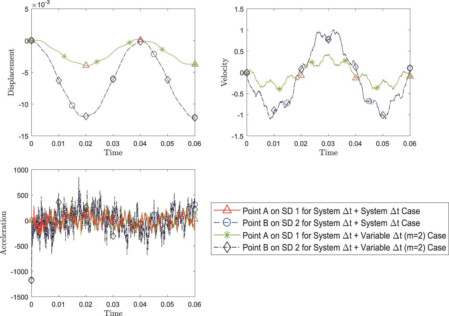
Figure 17: Comparison of transient response of displacement, velocity and acceleration at both point A and point B, between simulation with system Δt for both subdomains and with variable Δt = 1/2 system Δt for subdomain 2 while using FEM with implicit version (with η3 = 1) of GS4-II U0(1, 1, 0) algorithm for subdomain 1 and GPS with implicit version (with η3 = 1) U0(0, 0, 0) algorithm for subdomain 2
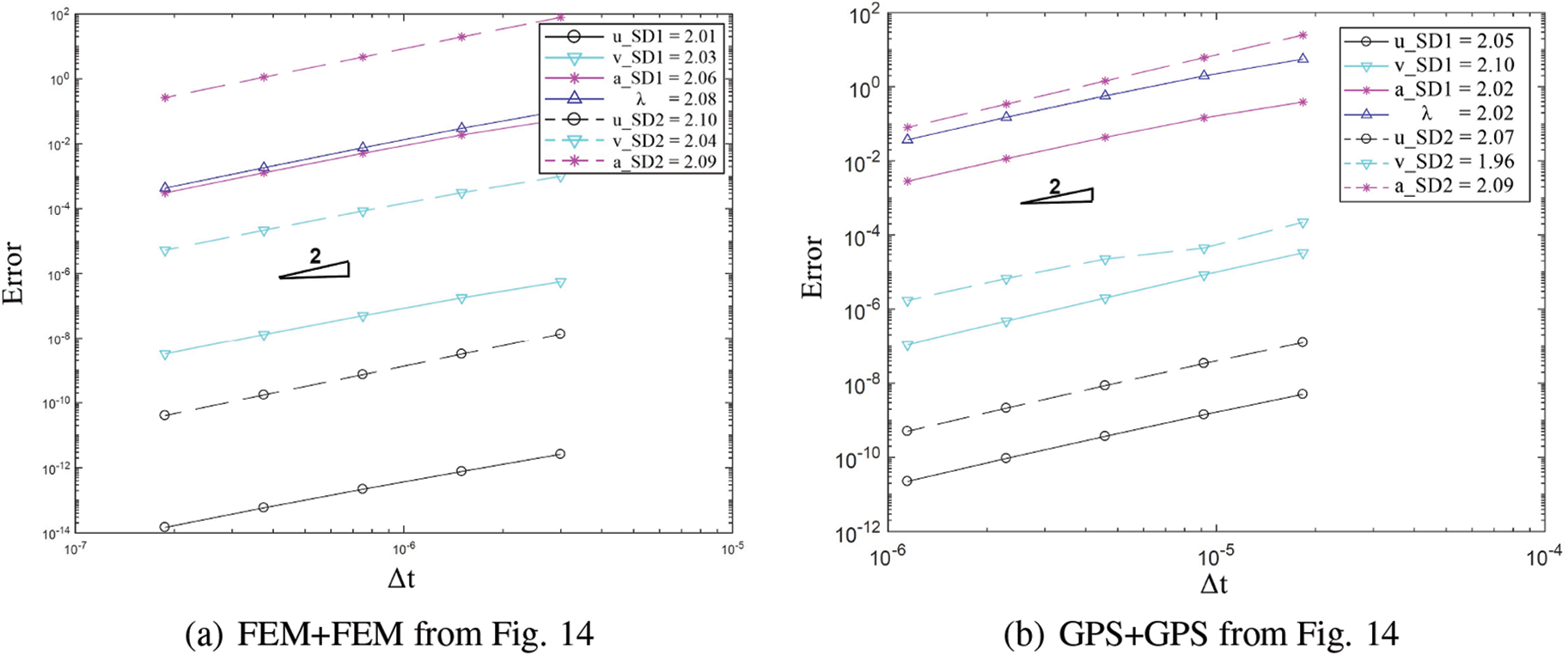
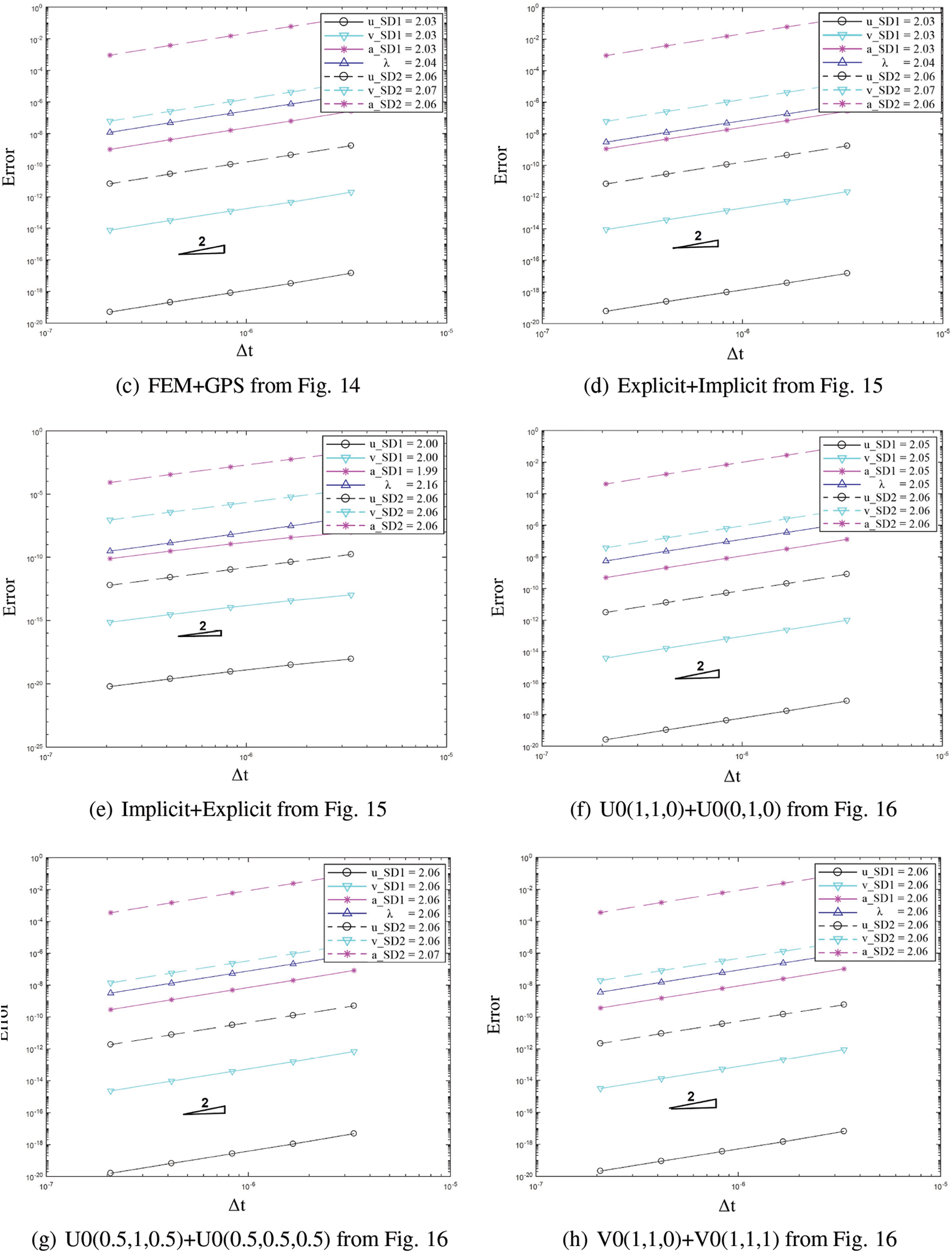
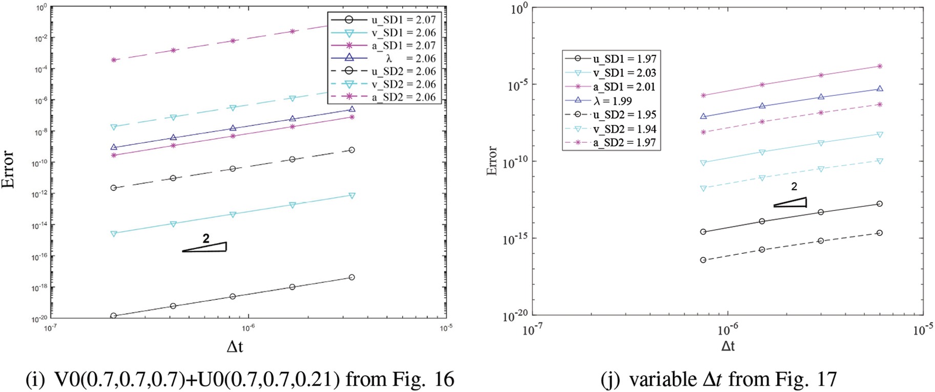
Figure 18: Convergence order for the solution with respect to the system time step for domain 1 and 2 in different cases: (a) FEM with implicit version of GS4-II U0(1, 1, 0) and FEM with U0(0, 0, 0), (b) GPS with implicit version of GS4-II U0(1, 1, 0) and GPS with U0(0, 0, 0), (c) FEM with implicit version of GS4- II U0(1, 1, 0) and GPS with U0(0, 0, 0), (d) FEM with explicit version of GS4-II U0(1, 1, 0) and GPS with implicit version U0(0, 0, 0), (e) FEM with implicit version of GS4-II U0(1, 1, 0) and GPS with explicit version U0(0, 0, 0), (f) FEM with implicit version of GS4-II U0(1, 1, 0) and FEM with U0(0, 1, 0), (g) FEM with implicit version of GS4-II U0(0.5, 1, 0.5) and GPS with U0(0.5, 0.5, 0.5) algorithm for subdomain 2, (h) FEM with implicit version of GS4-II V0(1, 1, 0) and GPS with V0(1, 1, 1), (i) FEM with implicit version of GS4-II V0(0.7, 0.7, 0.7) and GPS with V0(0.7, 0.7, 0.21), (j) variable Δt2 = 1/2 system Δt for subdomain 2 while using FEM with implicit version (with η3 = 1) of GS4-II U0(1, 1, 0) algorithm for subdomain 1 and GPS with implicit U0(0, 0, 0) algorithm for subdomain 2
5.3 2D Vibration Problem-Three Subdomains
Next, a body divided into three domains is examined next for the extension of the subdomain coupling concept. The same vibration problem above is evaluated again but this time, the beam is divided into three subdomains where
Figs. 20 and 21 clearly illustrate that the result at points A and B (shown in Fig. 19a) from the three subdomain case matches closely with the result from the two subdomain case while achieving second order time convergence rate. The high frequency in the acceleration plot for the three domain free end node is caused by the use of non-dissipative U0(1, 1, 0) scheme.
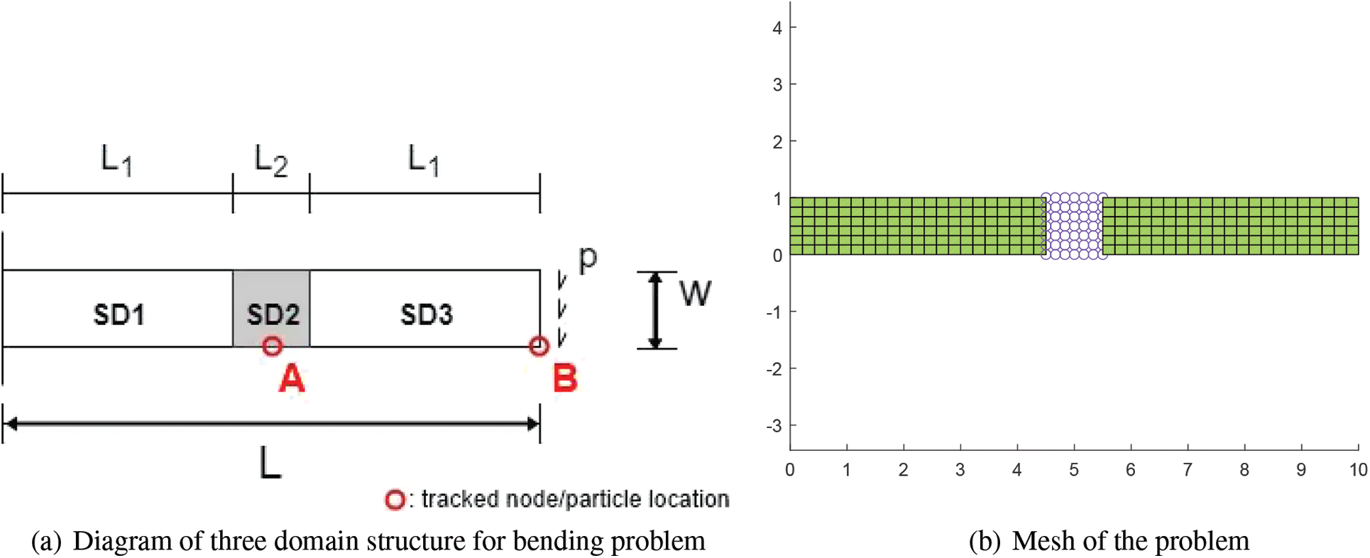
Figure 19: (a) Structure divided into three domains (b) An example of mesh of the structure: FEM GPS FEM
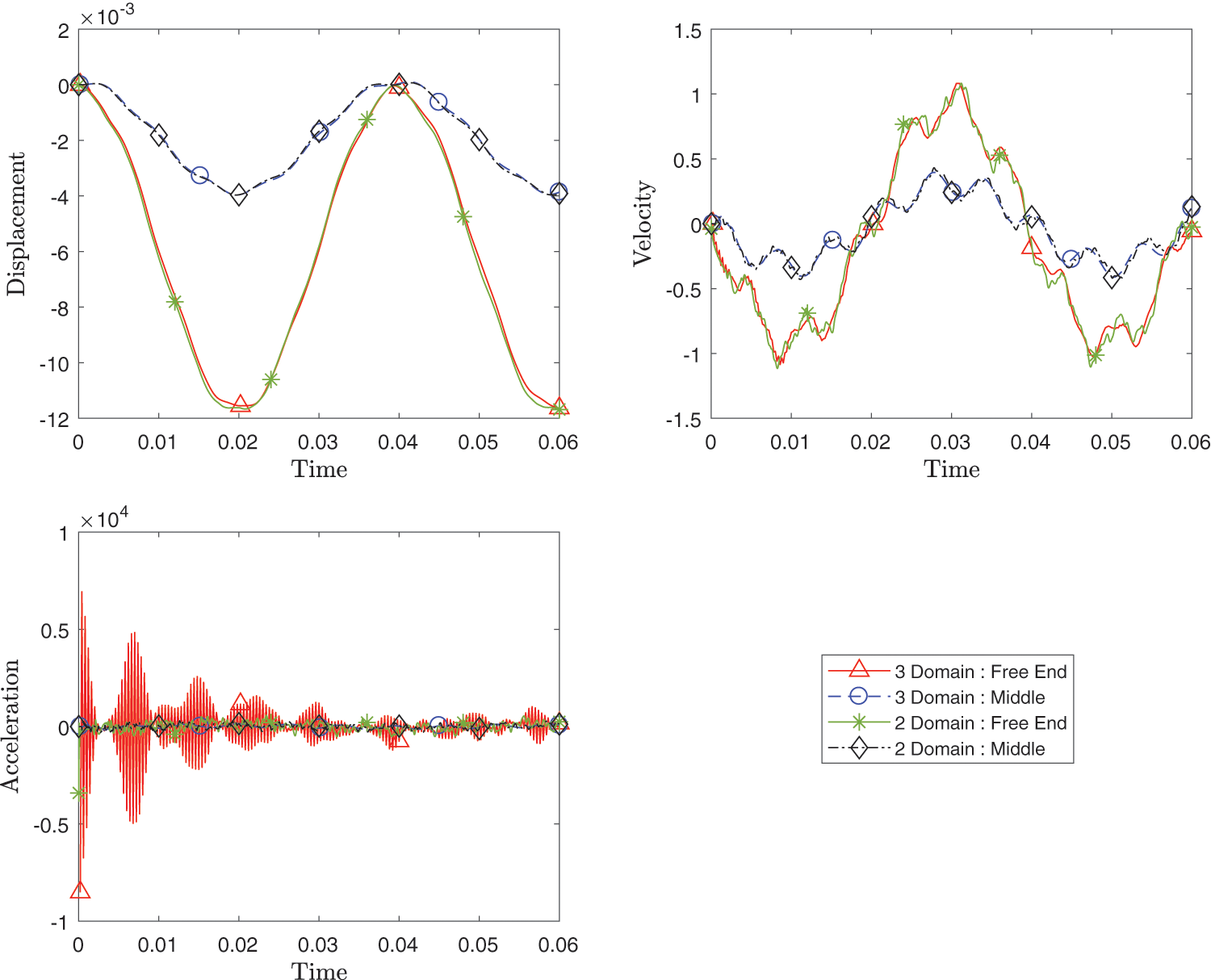
Figure 20: Comparison of transient response of displacement, velocity and acceleration at point A and point B between three subdomain configuration and two subdomain configuration while using FEM with implicit version (with η3 = 1) of GS4-II U0(1, 1, 0) algorithm for subdomain 1 and subdomain 3 and GPS with implicit version of U0(0, 0, 0) algorithm for subdomain 2 with constant Δt in all subdomains
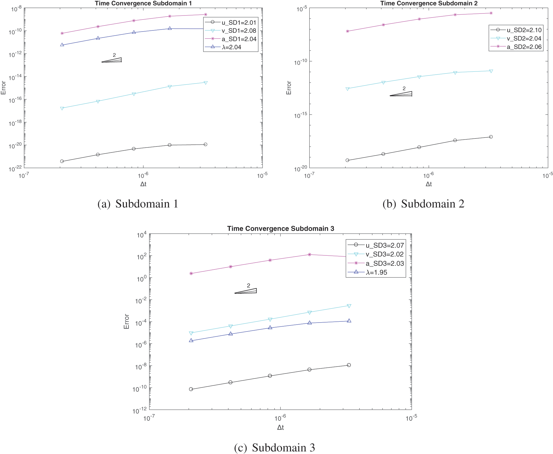
Figure 21: Convergence order for the solution with respect to the system time step for domain 1 and 2 and 3 in three domain configuration case: (a) subdomain 1 using FEM with implicit version of GS4-II U0(1, 1, 0) algorithm, (b) subdomain 2 using GPS with U0(0, 0, 0) algorithm, (c) subdomain 3 using FEM with GS4-II U0(1, 1, 0) algorithm
5.4 2D Notched Specimen Problem
Figs. 22 and 23 show the geometry of a 2D plane stress problem and an example of the mesh, respectively. It consists of three subdomains where identical subdomain 1 and 3 are connected by a thin subdomain 2. The subdomain 1 is 3 m by 2 m rectangle which are discretized into 176 FEM nodes. On the other hand, subdomain 2 is 1 m by 2 m rectangle bar, with notches on top and bottom, discretized into 99 particles. And subdomain 3 is identical to the subdomain 1 geometrically, but discretized with 176 particles. The whole geometry has thickness of 1 m. The semidiscrete equation of motion for the system is given as
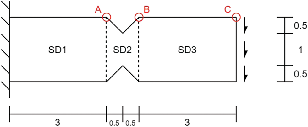
Figure 22: Diagram of structure divided into three subdomain. The red circles represent the locations where u,
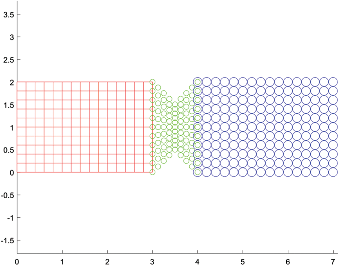
Figure 23: Mesh of all three subdomains
The bar is fixed at the left end and pulled down from the right end with a distributed load of 210 N/m. This material has 70 GPa for Young’s modulus, 0.3 for Poisson’s ratio, and
The time history of the y-direction displacement, velocity and acceleration of nodes/particles in each subdomain (points A, B, and C in Fig. 22) are evaluated.
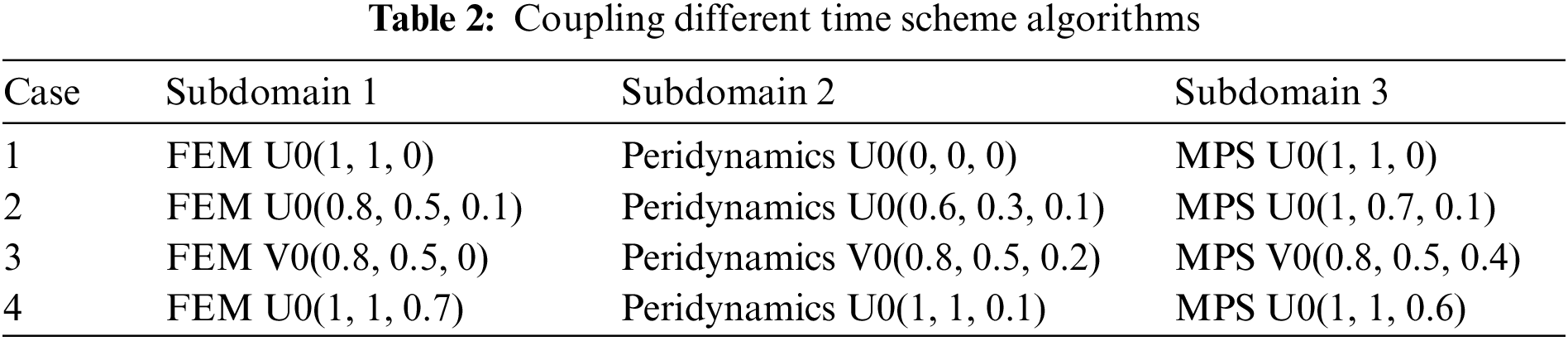
Figs. 24–26 show the transient response of the displacement, velocity and acceleration for points A, B and C for all cases listed in the Table 2 compared with the reference results. All responses from the different spatial methods and different time schemes combinations match well.
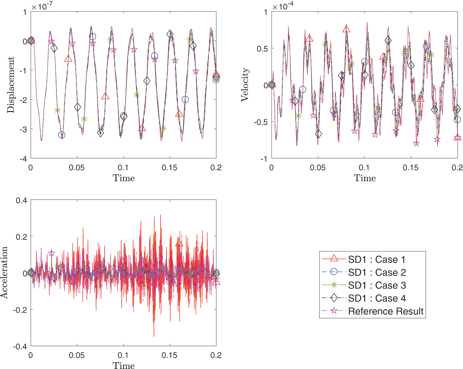
Figure 24: Comparison of transient response of displacement, velocity and acceleration at point A between different cases with varying method and time integration schemes for each domain as listed in Table 2
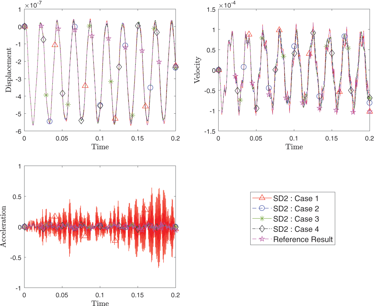
Figure 25: Comparison of transient response of displacement, velocity and acceleration at point B among different cases with varying method and time integration schemes for each domain as listed in Table 2
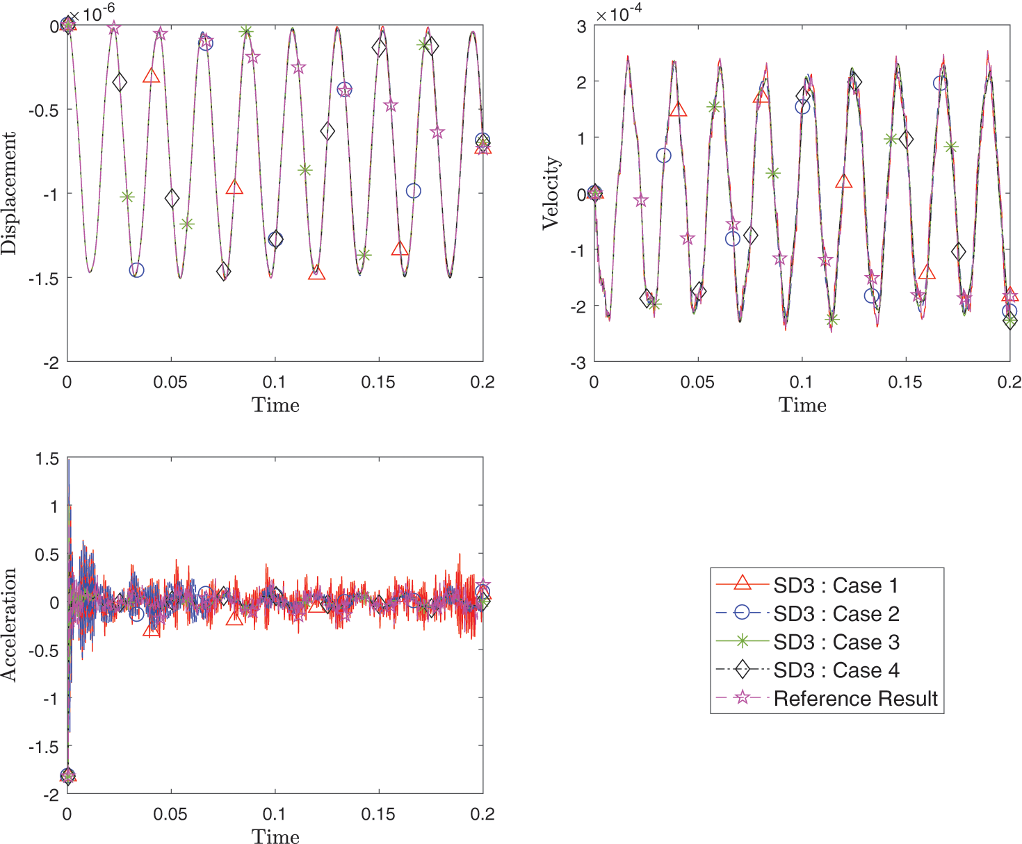
Figure 26: Comparison of transient response of displacement, velocity and acceleration at point C among different cases with varying method and time integration schemes for each domain as listed in Table 2
In this paper, we have proposed a novel implementation of the Generalized Single Step Single Solve time integration framework for ODE’s into the DAE framework. This proposed method, unlike traditional approaches in current technology with LMS methods, allows the coupling of different numerical analysis methods such as FEM and particle methods to be used on a single body while ensuring the accuracy of the result with the use of a wide variety of time integration algorithms within the GS4 framework. For example, one cannot simply or haphazardly couple the Midpoint rule with the Newmark method; or couple a multitude of schemes such as the Newmark, Midpoint rule, HHT, WBZ methods, etc., arbitrarily in different subdomains in a single analysis without loss and reduced accuracy in the convergence rate of one or more variables. However the GS4 framework circumvents various deficiencies, preserves accuracy, and permits a much broader design space for coupling algorithms in a single analysis and provides much desired robust features for applications to large scale industrial real world problems as well. It has the potential to increase the accuracy of the physics by selecting an appropriate method for only the area with a localized phenomena rather than utilizing only a single method that may not be suitable for certain applications on the whole body. The method is verified by applying it to 2D simple bar and beam problems. The results from various combination of methods and time scheme algorithms match closely with the reference result. With the basis of the proposed computational methodology established, the extension of the method for the future studies includes computational efficiency studies, extension to nonlinearity, and implementation of reduced order modeling. This work provides generality and versatility of the computational framework incorporating a wide variety of subdomain based spatial and time integration algorithms in a single analysis with great accuracy.
Funding Statement: The authors received no specific funding for this study.
Conflicts of Interest: The authors declare that they have no conflicts of interest to report regarding the present study.
1In this work, the weight function used in the weighted residual method is defined as C, and the weight function for describing the influence generated from neighboring particle is defined as W.
References
1. Gingold, R. A., Monaghan, J. J. (1977). Smoothed particle hydrodynamics: Theory and application to non-spherical stars. Monthly Notices of the Royal Astronomical Society, 181(3), 375–389. DOI 10.1093/mnras/181.3.375. [Google Scholar] [CrossRef]
2. Lucy, L. B. (1977). A numerical approach to the testing of the fission hypothesis. The Astronomical Journal, 82, 1013–1024. DOI 10.1086/112164. [Google Scholar] [CrossRef]
3. Benz, W. (1990). Smooth particle hydrodynamics: A review. In: The numerical modelling of nonlinear stellar pulsations, pp. 269–288. Dordrecht: Springer Netherlands. [Google Scholar]
4. Liu, G. R., Liu, M. B. (2003). Smoothed particle hydrodynamics: A meshfree particle method. Singapore: World Scientific. [Google Scholar]
5. Koshizuka, S., Oka, Y. (1996). Moving-particle semi-implicit method for fragmentation of imcompressible fluid. Nuclear Science and Engineering, 123, 421–434. DOI 10.13182/NSE96-A24205. [Google Scholar] [CrossRef]
6. Koshizuka, S., Nobe, A., Oka, Y. (1998). Numerical analysis of breaking waves using the moving particle semi-implicit method. International Journal for Numerical Methods in Fluids, 26, 751–769. DOI 10.1002/(ISSN)1097-0363. [Google Scholar] [CrossRef]
7. Silling, S. A. (2000). Reformulation of elasticity theory for discontinuities and long-range forces. Journal of the Mechanics and Physics of Solids, 48(1), 175–209. DOI 10.1016/S0022-5096(99)00029-0. [Google Scholar] [CrossRef]
8. Silling, S. A., Lehoucq, R. B. (2010). Peridynamic theory of solid mechanics, vol. 44. USA: Elsevier. [Google Scholar]
9. Seleson, P., Parks, M., Gunzburger, M., Lehoucq, R. B. (2009). Peridynamics as an upscaling of molecular dynamics. Multiscale Modeling & Simulation, 8(1), 204–227. DOI 10.1137/09074807X. [Google Scholar] [CrossRef]
10. Tae, D., Tamma, K. K. (2018). Mixed strong form representation particle method for solids and structures. Journal of Applied and Computational Mechanics, 4, 4, 429–441. [Google Scholar]
11. Ozaki, S., Hashiguchi, K., Okayasu, T., Chen, D. (2007). Finite element analysis of particle assembly-water coupled frictional contact problem. Computer Modeling in Engineering & Sciences, 18(2), 101–120. DOI 10.3970/cmes.2007.018.101. [Google Scholar] [CrossRef]
12. Bardenhagen, S. G., Kober, E. M. (2004). The generalized interpolation material point method. Computer Modeling in Engineering & Sciences, 5(6), 477–496. DOI 10.3970/cmes.2004.005.477. [Google Scholar] [CrossRef]
13. Sladek, J., Stanak, P., Han, Z., Sladek, V., Atluri, S. N. (2013). Applications of the MLPG method in engineering & sciences: A review. Computer Modeling in Engineering & Sciences, 92(5), 423–475. DOI 10.3970/cmes.2013.092.423. [Google Scholar] [CrossRef]
14. Li, J., Wang, X., Lee, J. D. (2012). Multiple time scale algorithm for multiscale material modeling. Computer Modeling in Engineering & Sciences, 85(5), 463–480. DOI 10.3970/cmes.2012.085.463. [Google Scholar] [CrossRef]
15. Orsini, P., Power, H., Lees, M. (2011). The hermite radial basis function control volume method for multi-zones problems; A non-overlapping domain decomposition algorithm. Computer Methods in Applied Mechanics and Engineering, 200(5), 477–493. DOI 10.1016/j.cma.2010.05.001. [Google Scholar] [CrossRef]
16. Metsis, P., Papadrakakis, M. (2012). Overlapping and non-overlapping domain decomposition methods for large-scale meshless EFG simulations. Computer Methods in Applied Mechanics and Engineering, 229, 128–141. DOI 10.1016/j.cma.2012.03.012. [Google Scholar] [CrossRef]
17. Park, K., Felippa, C. (2000). A variational principle for the formulation of partitioned structural systems. International Journal for Numerical Methods in Engineering, 47(1--3), 395–418. DOI 10.1002/(ISSN)1097-0207. [Google Scholar] [CrossRef]
18. Brezzi, F., Marini, L. (2005). The three-field formulation for elasticity problems. GAMM-Mitteilungen, 28(2), 124–153. DOI 10.1002/gamm.201490016. [Google Scholar] [CrossRef]
19. Xiao, S. P., Belytschko, T. (2004). A bridging domain method for coupling continua with molecular dynamics. Computer Methods in Applied Mechanics and Engineering, 193(17--20), 1645–1669. DOI 10.1016/j.cma.2003.12.053. [Google Scholar] [CrossRef]
20. Cundall, P. A., Peter, A., Strack, O. (1979). A discrete numerical model for granular assemblies. Geotechnique, 29(1), 47–65. DOI 10.1680/geot.1979.29.1.47. [Google Scholar] [CrossRef]
21. Morris, J., Rubin, M. B., Block, G. I., Bonner, M. P. (2006). Simulations of fracture and fragmentation of geologic materials using combined FEM/DEM analysis. International Journal of Impact Engineering, 33(1--12), 463–473. DOI 10.1016/j.ijimpeng.2006.09.006. [Google Scholar] [CrossRef]
22. Kozicki, J., Donze, F. V. (2008). A new open-source software developed for numerical simulations using discrete modeling methods. Computer Methods in Applied Mechanics and Engineering, 197(49--50), 4429–4443. DOI 10.1016/j.cma.2008.05.023. [Google Scholar] [CrossRef]
23. Macek, R. W., Silling, S. A. (2007). Peridynamics via finite element analysis. Finite Elements in Analysis and Design, 43(15), 1169–1178. DOI 10.1016/j.finel.2007.08.012. [Google Scholar] [CrossRef]
24. Kilic, B., Madenci, E. (2010). Coupling of peridynamic theory and the finite element method. Journal of Mechanics of Materials and Structures, 5(5), 707–733. DOI 10.2140/jomms. [Google Scholar] [CrossRef]
25. Zaccariotto, M., Mudric, T., Tomasi, D., Shojaei, A., Galvanetto, U. (2018). Coupling of FEM meshes with peridynamic grids. Computer Methods in Applied Mechanics and Engineering, 330, 471–497. DOI 10.1016/j.cma.2017.11.011. [Google Scholar] [CrossRef]
26. Gravouil, A., Combescure, A. (2001). Multi-time-step explicit-implicit method for non-linear structural dynamics. International Journal for Numerical Methods in Engineering, 50(1), 199–225. DOI 10.1002/(ISSN)1097-0207. [Google Scholar] [CrossRef]
27. Pegon, P. (2008). Continuous PsD testing with substructuring. In: Modern testing techniques for structural systems, pp. 197–257. Vienna: Springer Vienna. [Google Scholar]
28. Bursi, A. B. O. S., He, L., Magonette, G., Pegon, P. (2008). Convergence analysis of a parallel interfield method for heterogeneous simulations with dynamic substructuring. International Journal for Numerical Methods in Engineering, 75(7), 800–825. DOI 10.1002/nme.2285. [Google Scholar] [CrossRef]
29. Prakash, A., Hjelmstad, K. (2004). A FETI-based Multi-time-step Coupling Method for Newmark Schemes in Structural Dynamics. International Journal for Numerical Methods in Engineering, 61(13), 2183–2204. [Google Scholar]
30. Karimi, S., Nakshatrala, K. B. (2014). On multi-time-step monolithic coupling algorithms for elastodynamics. Journal of Computational Physics, 273, 671–705. DOI 10.1016/j.jcp.2014.05.034. [Google Scholar] [CrossRef]
31. Nakshatrala, K. B., Hjelmstad, K. D., Tortorelli, D. A. (2008). A FETI-based domain decomposition technique for time-dependent first-order systems based on a DAE approach. International Journal for Numerical Methods in Engineering, 75(12), 1385–1415. DOI 10.1002/nme.2303. [Google Scholar] [CrossRef]
32. Shimada, M. (2014). Novel design and development of isochronous time integration architectures for ordinary differential equations and differential-algebraic equations: Computational science and engineering applications (Ph.D. Thesis). The University of Minnesota-Twin Cities, Minneapolis, Minnesota, USA. [Google Scholar]
33. Maxam, D., Deokar, R., Tamma, K. K. (2019). A unified computational methodology for dynamic thermoelasticity with multiple subdomains under the GSSSS framework involving differential algebraic equation systems. Journal of Thermal Stresses, 42(1), 163–184. DOI 10.1080/01495739.2018.1536869. [Google Scholar] [CrossRef]
34. Tamma, K. K., Zhou, X., Sha, D. (2000). The time dimension: A theory towards the evolution, classification, characterization and design of computational algorithms for transient/dynamic applications. Archives of Computational Methods in Engineering, 7(2), 67–290. [Google Scholar]
35. Zhou, X., Tamma, K. (2006). Algorithms by design with illustrations to solid and structural mechanics/dynamics. International Journal for Numerical Methods in Engineering, 66(11), 1738–1790. DOI 10.1002/(ISSN)1097-0207. [Google Scholar] [CrossRef]
36. Zhou, X., Tamma, K. K. (2004). Design, analysis, and synthesis of generalized single step single solve and optimal algorithms for structural dynamics. International Journal for Numerical Methods in Engineering, 59, 597–668. DOI 10.1002/(ISSN)1097-0207. [Google Scholar] [CrossRef]
37. Har, J., Tamma, K. K. (2012). Advances in computational dynamics of particles, materials and structures. Chichester, UK: John Wiley & Sons. [Google Scholar]
38. Maxam, D. J., Tamma, K. K. (2022). A re-evaluation of overshooting in time integration schemes: The neglected effect of physical damping in the starting procedure. International Journal for Numerical Methods in Engineering, 123(12), 2683–2704. DOI 10.1002/nme.6955. [Google Scholar] [CrossRef]
Cite This Article
 Copyright © 2023 The Author(s). Published by Tech Science Press.
This work is licensed under a Creative Commons Attribution 4.0 International License , which permits unrestricted use, distribution, and reproduction in any medium, provided the original work is properly cited.
 Downloads
 Citation Tools