Genetic-Based Keyword Matching DBSCAN in IoT for Discovering Adjacent Clusters

1  Introduction

The spread of mobile devices and the development of network technology have spread IoT technology to various fields such as communication [1], home appliance [2], transportation [3], and healthcare [4]. Based on location information acquired through sensing technology, one of the core IoT technologies, various location-based services are provided in IoT environment [5]. Research to provide a new location-based service by finding useful information hidden in spatial data periodically collected from numerous mobile devices is being actively conducted [6].

Spatial clustering is one of the key technologies for analyzing spatial data, which is rapidly increasing due to the recent expansion of mobile devices and sensors [7]. Spatial clustering is used in the field of geographic data analysis such as crash & crime hotspots analysis [8,9], cartography [10], geographic segmentation of customers [11], earthquake area grouping [12], and commercial area analysis [13]. As the demand for spatial data analysis services increases, various analysis methods (nearest-neighbor searches on spatial data, nearest group queries, etc.) are being used [14,15]. Among the various spatial clustering algorithms, DBSCAN is one of the most widely used clustering algorithms [16].

DBSCAN has so far studied spatial data with numeric and categorical properties. However, spatial data collected in the real world includes textual data composed of natural language as well as formalized numerical or categorical data. For example, data for commercial area analysis has textual information (e.g., blog, website, user reviews) as well as location data of stores. The textual information in the spatial data can be a variety of text descriptions obtained from newspaper articles, personal blogs, and social networking services. For simplicity, we assume that textual information is a set of keywords such as tags. The existing clustering algorithms cannot utilize textual information. It is difficult to use textual information for commercial area analysis using a clustering algorithm. Therefore, there is a limit to processing various analysis techniques required for commercial area analysis with the existing clustering algorithms.

In commercial area analysis, it is important to identify areas where similar stores are concentrated in selecting the location of a new store to open, predicting expected sales of stores, and determining the convenience of the city. For example, if pharmacies are concentrated near an area where hospitals are concentrated, it is convenient for people who visit the hospital to go to the pharmacy after receiving prescriptions at the hospital. To make the example easier to understand, we define a set of data that is dense in space and has the same keyword in their textual information as a keyword-matching cluster. Fig. 1 shows the results of DBSCAN based on keywords for ‘hospital’ and ‘pharmacy’ (minPtr = 3). h1 and h2 are hospital dense areas, and d1 is a pharmacy dense area (data in both h1 and h2 have the ‘hospital’ keyword in their textual information, and data in d1 have the ‘pharmacy’ keyword in their textual information). However, in commercial area analysis, it can be useful not only to discover the area where keyword-matching clusters are concentrated but also to discover the keyword-matching clusters that are closest to each other among all keyword-matching clusters.

Figure 1: An example of results from keyword-matching DBSCAN

The distance between d1 and h1 is 1 km, and the distance between d1 and h2 is 7 km. In this case, the middle area (green area) between d1 and h1, which is close to both hospital and pharmacy dense areas, may be a suitable location for opening a new store that sells items conducive to patient health. In the commercial area analysis, it is an important task to discover the middle area between the two dense areas that are closest to each other. In this study, we define the keyword-matching clusters closest to each other as adjacent keyword-matching clusters. In Fig. 1, d1 and h1 are adjacent keyword-matching clusters. In spatial data analysis, the task to identify adjacent keyword-matching clusters can be used not only as a commercial area analysis but also as a measure of urban convenience. For example, the closer the hospital and pharmacy clusters are the more convenient life of the people who use medical services. The proximity of the two dense areas can be a criterion for grasping the convenience of the area. To the best of our knowledge, however, there has been no research on the algorithm for deriving clusters close to the keyword-based DBSCAN yet. In data analysis through clustering, it is necessary to set various hyperparameters to obtain an optimal result, and the results of the cluster are different for each setting.

Cluster results vary depending on the query keyword entered by the data analyst, and the textual of spatial data may change at any time. The clustering result may be continuously changed due to the change of the cluster algorithm parameter setting and the randomness of the query keyword by the data analyst. Therefore, it is impossible to index all cluster results for all cases. It is time-consuming to compare the results of all clusters to find the nearest cluster whenever the cluster results change.

In this paper, we propose a Genetic-based Keyword-Matching DBSCAN (GKM-DBSCAN) algorithm that can efficiently discover adjacent clusters in a keyword-based DBSCAN algorithm using genetic algorithms. For the first time, the brute force method can be considered as a method of finding the algorithms that are closest to each other. That is, all the distances between clusters derived for each keyword result set are calculated to find the closest set. The time complexity, in this case, is O(mq) where q is the number of query keywords by the user and m is the average number of clusters included in each keyword result set. To avoid the time complexity becoming an exponential function, we applied a genetic algorithm. To avoid constituting time complexity as an exponential function, we applied a genetic algorithm. In addition, we proposed an index number binarization (INB) method that increases the convergence speed by using the feature that chromosomes do not exceed the maximum cluster number in the genetic algorithm. The contributions of this paper are summarized as follows:

•   We proposed the novel problem of discovering a set of adjacent clusters among the cluster results derived for each keyword in the keyword-based DBSCAN algorithm.

•   We developed the GKM-DBSCAN algorithm to which the genetic algorithm was applied to discover the set of adjacent clusters among the cluster results derived for each keyword.

•   To improve the performance of GKM-DBSCAN, we improve the general genetic algorithm by adopting the index number binarization (INB) instead of the cluster number binarization (CNB).

•   We conducted extensive experiments on both real and synthetic datasets to show the effectiveness of GKM-DBSCAN over the brute-force method. The experimental results show that GKM-DBSCAN outperforms the brute-force method by up to 21 times. GKM-DBSCAN with INB is 1.8 times faster than GKM-DBSCAN with CNB.

The rest of this paper is organized as follows. Section 2 reviews work related to spatial clustering algorithms and keyword-matching clustering. In Section 3, we present the definition of the problem. In Section 4, we propose the genetic-based KM-DBSCAN algorithm. In Section 5, we present experimental results and their evaluation. In Section 6, we conclude our work and present some directions for future research.

2  Related Works

2.1 Data Collected in the IoT Environment

As IoT technology develops, various types of data are being collected. In the IoT environment, various sensors can typically collect traffic information [17,18] or obtain biometric information for healthcare services. Meng et al. [19] proposed a privacy-aware factorization-based hybrid method for healthcare service recommendation. The IoT is also being actively used in intelligent agricultural systems. Liu et al. [20] proposed a greenhouse climate prediction model using temperature, humidity, illuminance, carbon dioxide concentration, soil temperature, and soil humidity data. In the IoT environment, sensors can utilize the sensor’s location information along with the collected data, so it can be applied to location-based services. Liu et al. [21,22] proposed deep learning models that predict and recommend point-of-interests through location data.

2.2 Keyword-Matching DBSCAN

Recently, a vast amount of text data containing useful information is being generated through social network services or online news [23]. Xiong et al. [24] proposed a TextRank-based semantic clustering algorithm that extracts news keywords. Since text data is unstructured data, it has inherent incompleteness. Therefore, when analyzing text data using density-based clustering, it is necessary to properly handle missing values for the quality of clustering results. Xue et al. [25] proposed a new density-based clustering approach based on Bayesian theory to overcome the limitations of incomplete data.

As the scope of research is expanded so that DBSCAN can analyze data that includes textual data, a technique that can utilize textual data for clustering analysis is needed. To utilize texture data in clustering, a technique for efficiently retrieving data required for data analysis is preferentially needed. Generally, an inverted index is used to retrieve from a typical texture data [26]. An inverse index consists of several inverse lists including the IDs of all documents containing a word and its frequency. When a query is provided from a search user, the inverse list searches the inverse list for each word in the query to retrieve documents containing that word.

As the use of texture data increases in clustering that analyzes spatial data, research on an index structure that combines texture-based data search and spatial data indexing is also being actively conducted.

Cong et al. [27] and Rocha-Junior et al. [28] proposed an index structure that can process spatial data and texture data by integrating R-tree and inverse index. Yao et al. [29] proposed MHR-tree based on min-wise signature and linear hashing technique.

IR2-tree is a data structure improved to efficiently process texture data in R-tree that deal with spatial data. For this reason, IR2-tree is widely used in recent keyword search-based data mining that deals with spatial data and texture data at the same time [30]. Jang et al. [31] have demonstrated that IR2-tree is efficient for spatial data analysis including texture data using DBSCAN. We were also inspired by this solution and applied IR2-tree to DBSCAN and proposed a novel keyword-matching DBSCAN algorithm called KM-DBSCAN [31], which deals with textual information as well as numerical or categorical data.

KM-DBSCAN utilizes the IR2-tree as an index structure. To find keyword-matching objects in large datasets, it performs the nearest neighbor search in a branch and bound method. While traversing an IR2-tree, KM-DBSCAN effectively prunes unqualified nodes using both spatial and textual information of nodes. However, KM-DBSCAN only derives the results of all clusters that are dense with each keyword. Through the example in Table 1, we explain the operation method of KM-DBSCAN. If DBSCAN is performed with the data shown in Table 1, it can be divided into G1 and G2 according to the density of objects in Fig. 2.

Figure 2: An example of a keyword-matching tuple

Let D be an entire dataset consisting of tuples. A tuple is represented as <V, W>, V is a spatial data vector and W is a set of keywords. In Fig. 2, ɛ-neighborhood of o3 is {o4, o10} = {∀o∈D | dist(o3, o) ≤ ɛ }. The distance dist(oi, oj) between two tuples is calculated as the Euclidean distance between the tuple’s spatial data vectors. For example, o2.V = (10, 8) and o5.V = (12, 10). dist(o2, o5) = (10−12)2+(8−10)2 = 22. A keyword-matching ɛ-neighborhood of a tuple means the tuple that has the query keyword in a keyword set of the tuple in the ɛ-neighborhood of a tuple. A keyword-matching ɛ-neighborhood of o3 for keyword ‘coffee’ is {o4}. For example, given Q = {coffee, book} and minPts = 2, KM-DBSCAN derives C1 = {o1, o2}, C2 = {o3, o4}, C3 = {o5, o6} and C4 = {o7, o8} as a result. Fig. 2 shows the result of performing the KM-DBSCAN with ‘coffee’ and ‘book’ keywords.

2.3 DBSCAN Using Genetic Algorithm

A genetic algorithm is a search method that finds an optimal solution by mimicking the evolution of an organism while adapting to its environment.

Guan et al. [32] proposed a Particle swarm Optimized Density-based Clustering and Classification (PODCC) designed to offset the drawbacks of DBSCAN. Particle Swarm Optimization (PSO), a widely used Evolutionary and Swarm Algorithm, has been applied to optimization problems in different research domains including data analytics. In PODCC, a variant of PSO, SPSO-2011, is used to search the parameter space to identify the best parameters for density-based clustering and classification. PODCC can function in terms of both supervised and unsupervised learnings by applying the appropriate fitness functions proposed.

Mu et al. [33] proposed a parameter-free algorithm to perform DBSCAN with different density-level parameters. The results show that the proposed algorithm is capable of efficiently and effectively detecting clusters automatically with variable density levels. Compared with the original DBSCAN, the proposed algorithm can discover more noise points and its execution accuracy is higher.

Alajmi et al. [34] proposed the genetic algorithm and its alternative operator to find the most appropriate genetic algorithm set that obtains the optimum, or near optimum, solutions in a reasonable computational time. Twelve control parameter sets of binary encoded genetic algorithms are tested to solve unconstrained building optimization problems. The results show that population size is the most significant control parameter and that the crossover probability and mutation rate have insignificant effects on the genetic algorithm performance.

A genetic algorithm that finds an optimal solution is one of the meta-heuristic methodologies. However, most of the studies that applied the genetic algorithm to DBSCAN are studies that optimize the parameter value of the DBSCAN algorithm. To the best of our knowledge, there are no studies that search for the closest cluster among the clusters for each keyword. In this paper, we develop the Genetic algorithm-based Keyword Matching DBSCAN (GKM-DBSCAN) to which the genetic algorithm was applied to discover the set of adjacent clusters among the cluster results derived for each keyword.

3  Problem Definition

In this section, we provide some definitions and the problem to be solved in this study.

Definition 1 (keyword result set) R(k) is the set of keyword-matching clusters for the k-th keyword among given Q (1 ≤ k ≤ m). If n clusters are found as a result of KM-DBSCAN for the k-th keyword, it can be expressed as follows, R(k) = {C1, C2, …, Cn}. In our example, R(‘coffee’) = {C1, C2} and R(‘book’) = {C3, C4}.

Definition 2 (cluster minimum distance) The distance between the two elements with the shortest Euclidean distance among all pairs of elements is created by selecting one from each cluster for two clusters.

minD(Ci,Cj)=minD(oa,ob),∀oa∈Ci,∀ob∈Cj(1)

where D(oa, ob) is the Euclidean distance of the two objects oa and ob.

Definition 3 (cluster group) For all keyword result sets, a set containing as an element one cluster is selected from each keyword result set.

G={(C1,C2,…,Cm)|∀C1∈R1,∀C2∈R2,…,∀Cm∈Rm}(2)

In our example, the cluster group set G = {(C1, C3), (C1, C4), (C2, C3), (C2, C4)} is generated for 4 clusters (C1, C2, C3 and C4).

Definition 4 (inner distance of cluster group) The inner distance of clusters group is defined as the sum of the cluster minimum distances (minD) for all ordered pairs of elements in one cluster group, denoted by innerD(g), g ∈ G. In Fig. 3, if g = (C1, C2, C3), innerD(g) can be obtained as follows. innderD(g) = minD(C1, C2) + minD(C2, C3) + minD(C1, C3).

Figure 3: An example of the adjacent cluster

Definition 5 (adjacent cluster) Given the search keyword set Q, the adjacent cluster is defined as the cluster group with the shortest inner distance among the cluster group set G.

Problem. The purpose of this study is to find adjacent clusters among the keyword-matching clusters resulting from KM-DBSCAN.

Since several keyword-matching clusters can be derived for each keyword and the elements of the cluster group are composed of a combination of each keyword cluster, the number of elements in the cluster group may increase exponentially. The problem of finding an adjacent cluster can be viewed as finding an optimal solution among multiple solutions.

4  The Proposed Genetic Algorithm

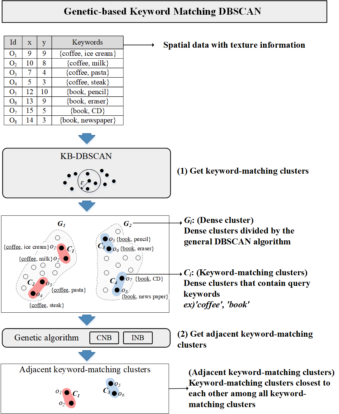
Before explaining the genetic algorithm proposed, we introduce an overall research framework. Our solution is to find the adjacent clusters from the keyword result set obtained from the result of KM-DBSCAN. (1) First, KB-DBSCAN is performed on spatial data with texture information to obtain a keyword result set. (2) In this study, we proposed a method to obtain adjacent keyword-matching clusters by applying two types of genetic algorithms (INB, CNB) to the keyword result set, which is the result of KB-DBSCAN. Fig. 4 shows an overall research framework.

Figure 4: An overall research framework

4.1 Chromosome Structure

In the genetic algorithm, the search is performed by applying selection, crossover, and mutation to the encoded individual through the encoding process that converts the possible solution of the problem into the form of a chromosome. The key point for finding an optimal solution by successfully using a genetic algorithm is how to construct a fitness function and how to encode a solution (chromosome). In genetic algorithms, the search is performed by applying selection, crossover, and mutation to the coded individual through the encoding process that converts the possible solution of the problem into the form of a chromosome. Depending on how a given problem is coded, the shape of the solution space changes, the applicable crossover or mutation method is different, and the search region created by the crossover or mutation method is also different. Therefore, for an efficient search, a solution expression method is important.

In general, in the case of genetic algorithms, the chromosome uses a one-dimensional array and the chromosome’s genetic factors are expressed in binary numbers. We constructed chromosomes with keyword-matching clusters included within cluster groups. The cluster number is converted to binary. The size of the chromosome is proportional to the number of search keywords Q.

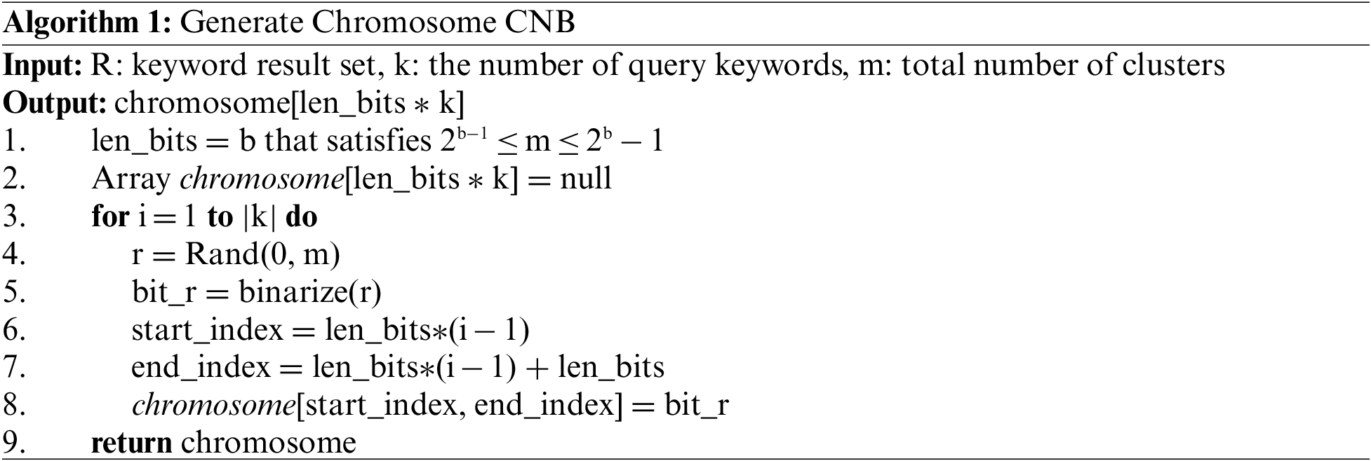
Assume that three keywords are given and the cluster group is configured as g = (C2, C4, C8). In Fig. 5, the cluster numbers are converted to binary numbers, and the converted binary numbers are concatenated in sequence. Algorithm 1 presents a method for generating an initial chromosome in a general genetic algorithm.

Figure 5: Structure of chromosome

4.2 Genetic Operations

In this study, we use the crossover and mutation operators as genetic operators. The traditionally used crossover operator creates a new combination of clusters using a two-point crossover for two chromosomes. In conventional mutation, it performs an operation by arbitrarily determining an arbitrary point in the chromosome and then converting the selected value to 1 if it is 0 and 0 if it is 1. In this way, the mutation operation enables the creation of various individuals by forcibly changing the value of a gene. Through these operations, it is expected that individuals with a better solution will be generated.

In our study, a problem arises in that offspring are generated inefficiently in crossover and mutation operations since the bits of the chromosome are constituted by the cluster number. For example, assume that the keyword result set is obtained as follows for two keywords. R1 = {C1, C4, C6, C10, C15} and R2 = {C3, C7, C8}. The largest cluster number in R1 is 15, and the largest cluster number in R2 is 8. At least 4 bits can represent 8 and 15. Since a chromosome is composed of two keyword results, the maximum length of a chromosome is 8 bits. An initial chromosome is constructed by randomly selecting one cluster from each keyword result. Fig. 6 shows the configuration of chromosomes (0001|0011) by selecting C1 from R1 and C3 from R2.

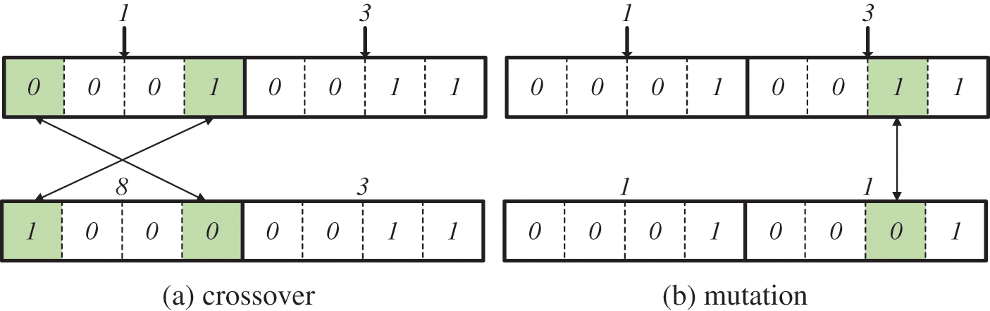
Figure 6: Inefficient offspring generation (a) crossover (b) mutation

Fig. 6 shows that the offspring generated through the crossover operation and the mutation operation is inefficient when chromosomes are constructed by cluster numbers. In Fig. 6a, the 1st and 4th genes are selected through the crossover operation and exchanged, and a new offspring (1000|0011) is generated. The group set (C8, C3) is obtained by converting offspring to cluster numbers for fitness evaluation. According to Definition 11, only the cluster included in R1 can be included in the first element of the groupset. Since C8 is not included in R1, the newly generated offspring does not need to calculate the fitness. The inclusion of chromosomes that do not require fitness calculations in the next generation increases time costs by generating unnecessary fitness evaluation calculations. This problem also appears in mutation operations. In Fig. 6b, the 7th gene is selected and changed from 0 to 1 through mutation operation, and a new offspring (0001|0001) is generated. The group set (C1, C1) is obtained by converting offspring to cluster numbers for fitness evaluation. According to Definition 11, only the cluster included in R2 can be included in the second element of the groupset. Since C1 is not included in R2, the newly generated offspring does not need to calculate the fitness.

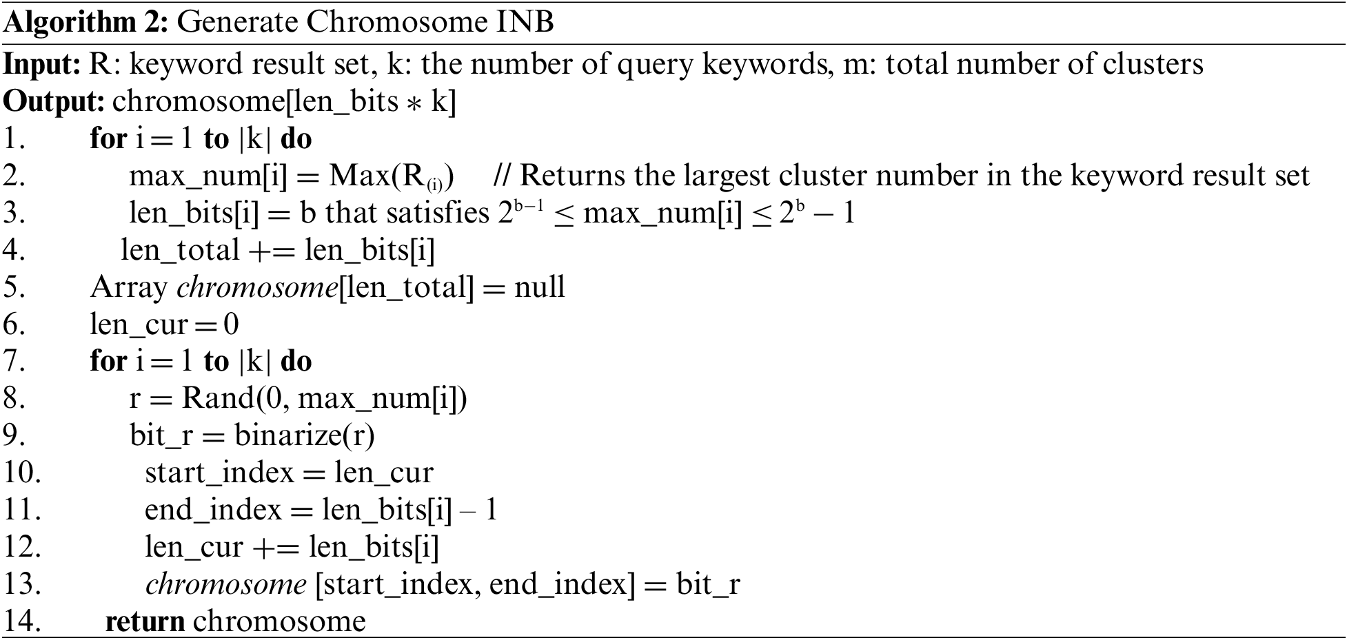
In this paper, instead of the cluster number binarization (CNB), we propose an index number binarization (INB) for configuring chromosomes by assigning an index to each cluster included in the cluster group and binarizing the index value. Algorithm 2 presents a method for generating early chromosomes in a genetic algorithm using CNB.

Index number binarization is performed in the following way. First, a list is created as many as the number of elements in the keyword result set. In our example, two keyword results (R1, and R2) are included in the keyword result set. The list stores the address of the index table. The index table contains clusters and index numbers included in one keyword set. In Fig. 7, the list of length 2 is created. An index table is created for each keyword result. For R1 = {C1, C4, C6, C10, C15}, each cluster in R1 is sequentially included in the index table along with the index value. Index values are sequentially assigned to the cluster from 0 and increasing by 1.

Figure 7: Index number binarization

In Fig. 7, the highest number of indices allocated to the cluster included in R1 is 4. Because a positive integer m has b bits when 2b−1 ≤ m ≤ 2b − 1, the minimum number of bits required to represent 4 with 2 bits is 3. The minimum number of bits in R2 is 2. An initial chromosome is constructed by randomly selecting one cluster from each keyword result. For initial chromosomal construction, C6 was selected in R1 and C7 was selected in R2. Index value 2 of C6 and index value 1 of C7 are binarized to form chromosomes (010|01). INB does not have an empty number in the middle because the index value increases sequentially from 0 to the maximum value. Therefore, the probability of generating an invalid offspring is low (see Fig. 8).

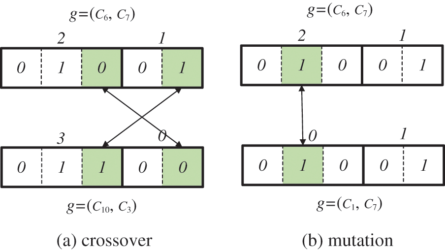
Figure 8: Genetic operation (a) crossover (b) mutation

However, this does not mean that invalid offspring is not generated even in INB. Up to 2b − 1 can be expressed with b bits. For example, 000, 001, 010, 011, 100, 101, 110, 111 can be expressed with 3 bits. However, since the maximum index is 4 (100), if a chromosome is composed of a bit (101, 110, 111) greater than the maximum index value, the chromosome becomes an invalid chromosome (see Fig. 9). Even in this case, it is a chromosome that does not need to calculate fitness.

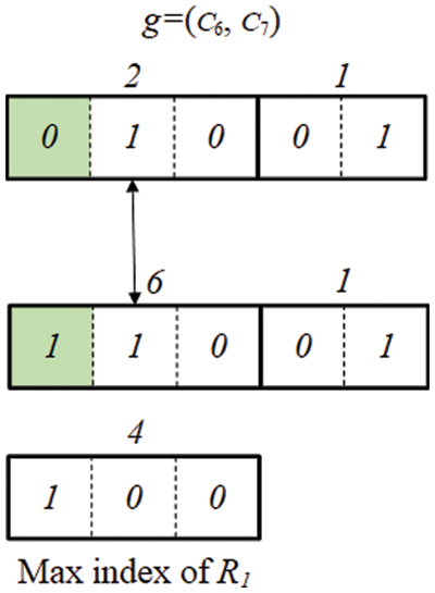
Figure 9: Example of an eliminated chromosome in INB

We utilize the maximum value of the cluster index to avoid calculating the fitness for invalid chromosomes. Since the maximum index value for each cluster group is known, if the value generated by the genetic operation is greater than the maximum value, the chromosome is eliminated without calculating the fitness. In Fig. 9, since the maximum index value of R1 is 4 (100), if the value generated by the mutation is 6 (110), this chromosome does not perform a fitness calculation. Although INB also generates invalid offspring, we prove that CNB is approximately twice as likely to generate invalid offspring as INB in Appendix A.

4.3 Objective Function

The objective function is a criterion for judging how close the current generation is to the solution, and it determines the overall performance of the genetic algorithm. In this study, the objective function is to measure the shortest inner distance of the cluster group such as Eq. (3).

fit(g)=innerD(g)(3)

where g is a cluster group. The innerD function is presented in Definition 4.

4.4 Design of Genetic Algorithm

The process of the genetic algorithm is shown in Fig. 10. Given data D and a query keyword Q, we first obtain keyword result sets for each keyword by performing KM-DBSCAN. Our genetic algorithm begins with the initial population. Chromosomes of the initial population are generated by combining randomly selected clusters from each keyword result set. The fitness is evaluated for the chromosomes constituting the initial population. In this study, we use a ranking selection strategy. Chromosomes in a list are sorted according to their fitness. The position of the chromosome in the list means a ranking. By selecting the top-ranking k, the genetic algorithm is applied and the next generation is generated.

Figure 10: Flowchart of genetic algorithm

The crossover operation is an operation that enables the generation of various individuals that do not exist in the population by exchanging information possessed by individuals. Therefore, it is expected that the chromosome with a better solution will be generated through the crossover operation. In general, a crossover operation is performed by exchanging a portion of a gene between chromosomes, and various crossover operations can be defined depending on the type of the encoded chromosome. We adopted a simple crossover that randomly determines one crossover point for a pair of individuals and exchanges each other around the crossover point.

As the population progresses from generation to generation, the child chromosomes become more similar to the population. Therefore, even if the cross operation is performed, it may not be possible to generate a new chromosome. The mutation operation is performed to compensate for the limitations of the crossover operation. A mutation operation is performed by determining an arbitrary point in the chromosome and changing the selected value to 1 if it is 0 and to 0 if it is 1. Mutation operation enables the generation of various chromosomes by forcibly changing the value of a gene. However, if the ratio of mutation operation is too large, the probability of the mutation in the direction of low fitness will also increase, and the solution will be difficult to obtain.

4.5 Computational Complexity Analysis

Given q keywords from the user, a q keyword result set is obtained. Assume that the total number of clusters is m. To find a solution using the brute-force approach without using a genetic algorithm, the inner distances of all cluster groups must be calculated. In the brute-force approach, if the average number of clusters in each keyword set is m/q, the number of cluster combinations to be calculated to find adjacent clusters is (m/q)q.

The computational complexity of the proposed genetic algorithm includes encoding and calculating fitness. A chromosome is generated by selecting one cluster from the q keyword result sets, and the number of chromosomes in one generation is the population size, p. If the number of trials to find the optimal solution is t, the time complexity of the proposed genetic algorithm is O(p*q*t).

5  Evaluations

5.1 Experiment Setting

Algorithm. In this study, we defined a new problem to find adjacent clusters in the keyword result set. Therefore, there is still no existing algorithm that can directly solve this problem. Therefore, first of all, we set the brute force approach as the baseline, which is the most basic approach to finding the optimal solution. Therefore, first of all, we set the brute force approach as the baseline, which is the most basic approach to finding the optimal solution. Next, a general genetic algorithm was applied to show that the genetic algorithm can solve our problem efficiently. It was shown that the CNB method proposed in this study is more suitable for solving our problem than the INB method used in the general genetic algorithm.

In this section, we compared our GKM-DBSCAN algorithm with not only the original genetic algorithm but also the brute-force approach by varying several parameters. Our GKM-DBSCAN algorithm finds the adjacent cluster with a genetic algorithm using INB and the original genetic algorithm (General) finds the adjacent cluster with a genetic algorithm using CNB based on the keyword result sets obtained by KM-DBSCAN. The brute-force (BF) approach finds the adjacent cluster by calculating all combinations of cluster groups without using a genetic algorithm.

Datasets. We used real and synthetic datasets for experiments. Real datasets are collected from data.world (https://data.world/datasets/geospatial). Each tuple in real datasets has longitude and latitude coordinates as spatial data. We need not only spatial data for each tuple but also purchase item data for experiments. Purchase item data was arbitrarily added to the real data with spatial data. To eliminate the problem of bias in spatial data, we normalized spatial data into the space (0, 0) × (10, 10 K).

To evaluate the effects of various parameters, we additionally generated a synthetic dataset with Gaussian distribution in the space. The synthetic dataset has various cardinalities N in the range [10, 200 k]. To get the keyword result sets with KM-DBSCAN, we set ɛ to 30 and minPtr to 3, which are required parameters in DBSCAN. Table 2 presents the algorithm parameters we used in our experiments, and default values are shown in boldface. All experiments were repeated 10 times and the average value was measured.

We implemented all algorithms using Java. Experiments were conducted on a Windows 7 platform using 32 GB of memory, 3.50 GHz, and Intel Core i7. When performing KM-DBSCAN, IR2-tree was used for data indexing. The page size of a node on the IR2-tree was 4096 bytes.

5.2 Effect of Data Size and Number of Keywords

In this section, we evaluate the scalability concerning the cardinality N of the dataset and the number of keywords. We conduct experiments with various cardinalities N[10, 200 k] and k[2, 8]. Fig. 11 shows the experiments for varying N. As shown in Fig. 11, GKM-DBSCAN generally outperforms the BF method and General method in all datasets. The performance difference increases as the cardinality increases. This shows that GKM-DBSCAN algorithm performs effectively for a large dataset. As the number of keywords increases, it can be seen that the difference between BF and the others (GKM-DBSCAN and General) becomes wider. As shown in Figs. 11a and 11d, we can see the difference in time cost between BF and the others with the number of keywords, 2 and 8, in the case of a data size of 200 k. The difference in time cost is about 1.2 times in the number of keywords 2, whereas the difference in time cost is 21 times in the number of keywords 8. As shown in the computational complexity analysis, the brute-force method, which is not based on a genetic algorithm, has the number of keywords as an exponent in the time complexity. Thus, as the number of keywords increases, time complexity increases exponentially.

Figure 11: Effects of data size and the number of keywords

5.3 Effect of the Population Size

In this section, we compare a genetic algorithm based on two algorithms, GKM-DBSCAN and General to evaluate the performance according to the genetic algorithm parameters. The size of the population affects the convergence speed and time cost. We evaluate the effect of the population size. We conduct experiments with various population sizes p[50, 100, 150, 200, 250, 300, 350, 400, 450, 500]. Fig. 12 shows the experiments for varying p. GKM-DBSCAN generally outperform General in all datasets. In our experiments, the time cost decreases until the population size is 400, and increases slightly from 400. In general, as the population increases, the amount of genetic operations increases accordingly, so the number of operations performed in one generation increases. However, as the population size increases, the probability of finding an optimal solution increases, and the speed of convergence increases. When the population is between 50 and 400, the convergence speed increases faster than the increase in the amount of computation in one generation, and the total time cost decreases. However, as the population size becomes more than 400, the amount of computation in one generation is greater than the convergence speed, increasing the total time cost.

Figure 12: Effect of population size (a) in the synthetic dataset (b) real data

5.4 Convergence Speed

In this section, we evaluate the convergence speed. Fig. 13 presents the graph comparing the degree of fitness change by generation in GAs. GKM-DBSCAN converges to a certain value when the generation value reaches 50 if the fitness value rapidly decreases initially as generations increase. In contrast, the reduction rate of general is slow and the generation value reaches 70. This means that INB is shown to improve the convergence speed to find the optimal solution.

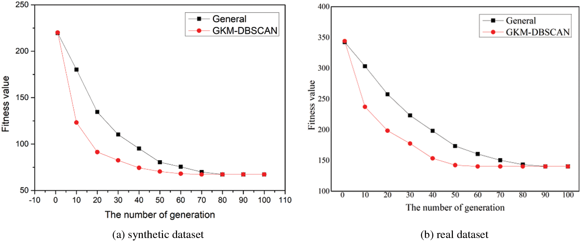
Figure 13: Convergence speed (a) in the synthetic dataset (b) real data

5.5 Length of Chromosome

In this section, we evaluate the length of chromosomes concerning the number of clusters. We conduct experiments with various cardinalities m[100, 8000]. Fig. 14 shows the experiments for varying m. As the number of clusters m increases, the maximum cluster number that each cluster group can have increased. Therefore, as the number of clusters increases, the length of the chromosome increases. Of course, the clusters included in the cluster group may vary depending on the data to be analyzed. It can be seen that the chromosome length of INB is shorter than that of CNB. Our experiments show that the length of the chromosome in INB is average 1.625 bits shorter than in CNB.

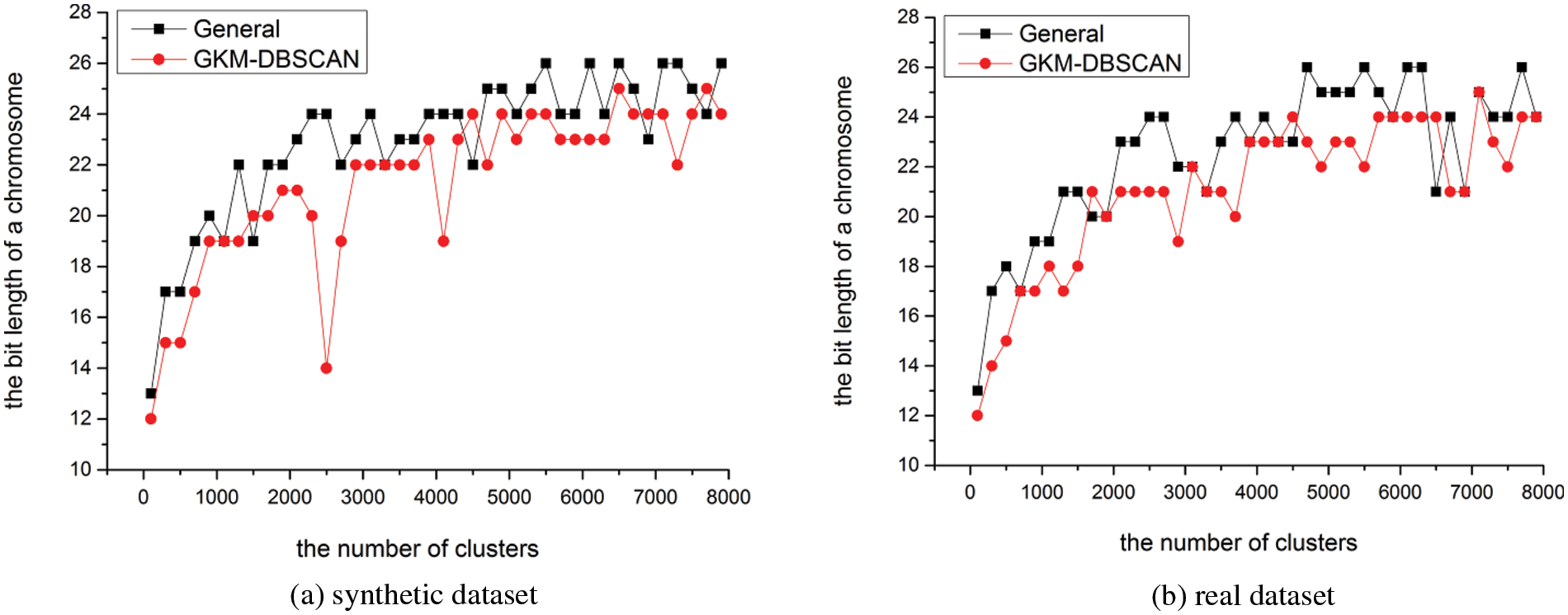
Figure 14: Length of chromosome (a) in the synthetic dataset (b) real data

5.6 Ratio of Invalid Chromosomes

In this section, we evaluate the ratio of invalid chromosome generation respect to the number of clusters. We conduct experiments with various cardinalities m[100, 8000]. Fig. 15 shows the experiments for varying m. We set the number of chromosomes constituting one generation to 400 (population size). 400 chromosomes are newly generated by genetic operation, and the ratio of invalid chromosomes was measured as the number of invalid chromosomes among them. In Fig. 15, as the number of clusters increases, the length of the chromosome increases, and as the length of the chromosome increases, the probability of generating an invalid chromosome increases. However, as the number of clusters increases, it can be seen that the increased amount of probability in CNB is larger than in INB. In Fig. 15, the ratio is measured as the probability in CNB divided by the probability in INB. As seen in Lemma 1, it can be seen that this ratio converges to 2 as the number of clusters increases.

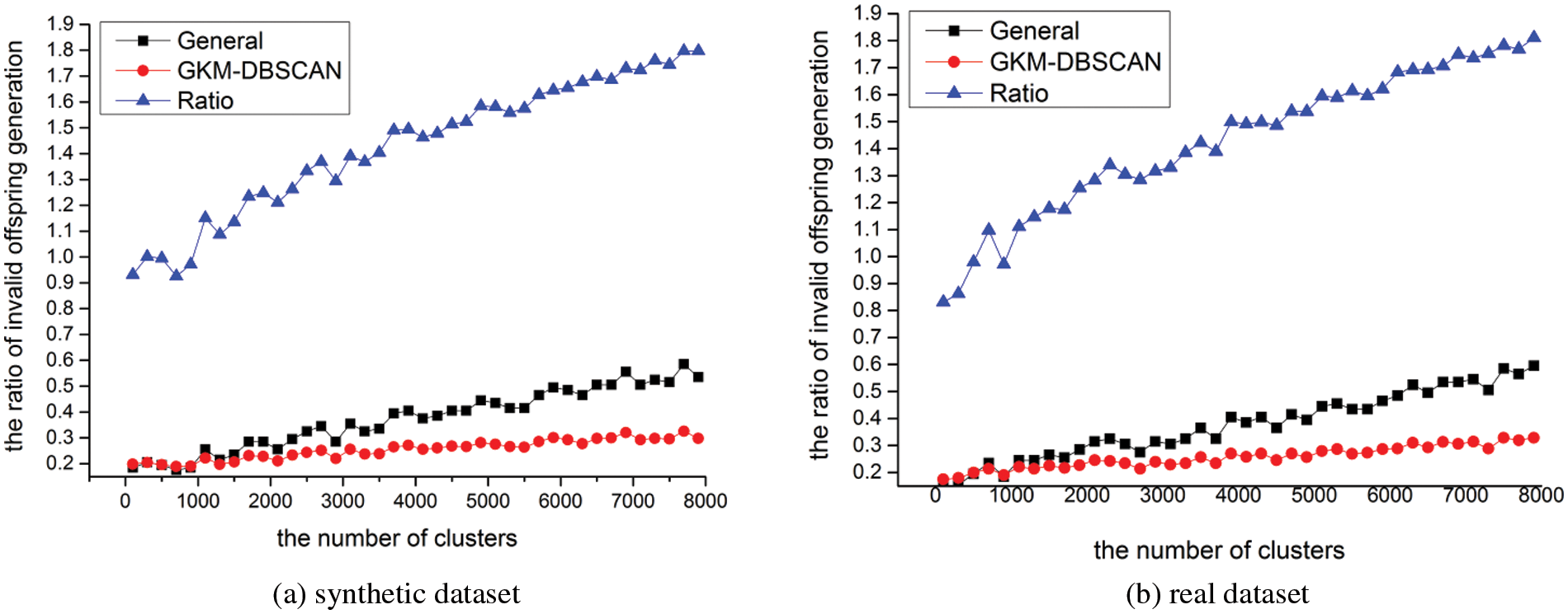
Figure 15: Ratio of invalid chromosomes (a) in synthetic dataset (b) real data

6  Conclusion

This paper defines the novel problem of discovering a set of adjacent clusters among the cluster results derived for each keyword in the KM-DBSCAN algorithm. To solve this problem, we first proposed the GKM-DBSCAN algorithm, to which the genetic algorithm was applied to discover the set of adjacent clusters among the cluster results derived for each keyword. To improve the performance of GKM-DBSCAN, we adopted the index number binarization instead of the cluster number binarization. We conducted extensive experiments on both real and synthetic datasets to show the effectiveness of GKM-DBSCAN over the brute-force method. The experimental results show that GKM-DBSCAN outperforms the brute-force method by up to 21 times. GKM-DBSCAN with the index number binarization is 1.8 times faster than GKM-DBSCAN with the cluster number binarization. In our experimental data, the data were evenly distributed. However, when the distribution of data is skewed, the disadvantage is that the difference between CNB and INB may be similar. This is because chromosomes become similar in size when each keyword result set has a large number of cluster numbers. In future work, we plan to extend our proposal to deal with not only uniform and Gaussian distribution but also skewed data distribution and to consider an optimized keyword-matching DBSCAN algorithm in a parallel processing environment.

Acknowledgement: The authors wish to express their appreciation to the reviewers for their helpful suggestions which greatly improved the presentation of this paper.

Funding Statement: This research was supported by the Basic Science Research Program through the National Research Foundation of Korea (NRF) funded by the Korea government (MSIT) (No. 2021R1F1A1049387).

Conflicts of Interest: The authors declare that they have no conflicts of interest to report regarding the present study.

References

 1.  Rahimi, H., Zibaeenejad, A., Safavi, A. A. (2018). A novel IoT architecture based on 5 G-IoT and next generation technologies. 2018 IEEE 9th Annual Information Technology, Electronics and Mobile Communication Conference (IEMCON), pp. 81–88. Vancouver, BC, Canada. [Google Scholar]

 2.  Asaithambi, S. P. R., Venkatraman, S., Venkatraman, R. (2021). Big data and personalisation for non-intrusive smart home automation. Big Data and Cognitive Computing, 5(6), 1–21. DOI 10.3390/bdcc5010006. [Google Scholar] [CrossRef]

 3.  Shukla, S., Balachandran, K., Sumitha, V. S. (2016). A framework for smart transportation using big data. 2016 International Conference on ICT in Business Industry & Government (ICTBIG), Indore, India. [Google Scholar]

 4.  Bhatia, H., Panda, S. N., Nagpal, D. (2020). Internet of things and its applications in healthcare--A survey. 2020 8th International Conference on Reliability, Infocom Technologies and Optimization (Trends and Future Directions) (ICRITO), Noida, India. [Google Scholar]

 5.  Carvalho, M. A., Silva, J. N. (2019). RConnected middleware: Location based services for IoT environments. 2019 Sixth International Conference on Internet of Things: Systems, Management and Security (IOTSMS), Granada, Spain. [Google Scholar]

 6.  Quezada-Gaibor, D., Klus, L., Torres-Sospedra, J., Lohan, E. S., Nurmi, J. et al. (2020). Improving DBSCAN for indoor positioning using Wi-fi radio maps in wearable and IoT devices. 2020 12th International Congress on Ultra Modern Telecommunications and Control Systems and Workshops (ICUMT), Brno, Czech Republic. [Google Scholar]

 7.  Liu, Q., Deng, M., Shi, Y., Wang, J. (2012). A density-based spatial clustering algorithm considering both spatial proximity and attribute similarity. Computers & Geosciences, 46, 296–309. DOI 10.1016/j.cageo.2011.12.017. [Google Scholar] [CrossRef]

 8.  Khosrowshahi, A. G., Aghayan, I., Kunt, M. M., Choupani, A. A. (2021). Detecting crash hotspots using grid and density-based spatial clustering. Proceedings of the Institution of Civil Engineers-Transport, pp. 1–13. DOI 10.1680/jtran.20.00028. [Google Scholar] [CrossRef]

 9.  Estivill-Castro, V., Lee, I. (2002). Multi-level clustering and its visualization for exploratory spatial analysis. GeoInformatica, 6(2), 123–152. DOI 10.1023/A:1015279009755. [Google Scholar] [CrossRef]

10. Li, Z. (2006). Algorithmic foundation of multi-scale spatial representation. Florida, USA: CRC Press. [Google Scholar]

11. Miller, H. J., Han, J. (2009). Geographic data mining and knowledge discovery. Florida, USA: CRC Press. [Google Scholar]

12. Mustakim, Rahmi, E., Mundzir, M. R., Rizaldi, S. T., Okfalisa et al. (2021). Comparison of DBSCAN and PCA-DBSCAN algorithm for grouping earthquake area. 2021 International Congress of Advanced Technology and Engineering (ICOTEN), Taiz, Yemen. [Google Scholar]

13. Fu, D., He, S. (2016). New combination algorithms in commercial area data mining and clustering. 2016 IEEE International Conference on Big Data Analysis (ICBDA), Hangzhou, China. [Google Scholar]

14. Jang, H. J., Hyun, K. S., Chung, J., Jung, S. Y. (2020). Nearest base-neighbor search on spatial datasets. Knowledge and Information Systems, 62(3), 867–897. DOI 10.1007/s10115-019-01360-3. [Google Scholar] [CrossRef]

15. Choi, D. W., Chung, C. W. (2015). Nearest neighborhood search in spatial databases. 2015 IEEE 31st International Conference on Data Engineering, pp. 699–710. Seoul, Korea (South). [Google Scholar]

16. Ester, M., Kriegel, H. P., Sander, J., Xu, X. (1996). A density-based algorithm for discovering clusters in large spatial databases with noise. Proceedings of the Second International Conference on Knowledge Discovery and Data Mining, pp. 226–231. Portland, USA. [Google Scholar]

17. Wang, F., Li, G., Wang, Y., Rafique, W., Khosravi, M. R. et al. (2022). Privacy-aware traffic flow prediction based on multi-party sensor data with zero trust in smart city. ACM Transactions on Internet Technology. DOI 10.1145/3511904. [Google Scholar] [CrossRef]

18. Qi, L., Wang, F., Xu, X., Dou, W., Zhang, X. et al. (2022). Time-aware missing traffic flow prediction for sensors with privacy-preservation. In: Liu, Q., Liu, X., Chen, B., Zhang, Y., Peng, J. (Eds.Lecture notes in electrical engineering. vol. 808, Singapore: Springer. DOI 10.1007/978-981-16-6554-7_78. [Google Scholar] [CrossRef]

19. Meng, S., Fan, S., Li, Q., Wang, X., Zhang, J. et al. (2022). Privacy-aware factorization-based hybrid recommendation method for healthcare services. IEEE Transactions on Industrial Informatics, 18(8), 5637–5647. DOI 10.1109/TII.2022.3143103. [Google Scholar] [CrossRef]

20. Liu, Y., Li, D., Wan, S., Wang, F., Dou, W. et al. (2021). A long short-term memory-based model for greenhouse climate prediction. International Journal of Intelligent Systems, 37(1), 135–151. DOI 10.1002/int.22620. [Google Scholar] [CrossRef]

21. Liu, Y., Pei, A., Wang, F., Yang, Y., Zhang, X. et al. (2021). An attention-based category-aware GRU model for the next POI recommendation. International Journal of Intelligent Systems, 36(7), 3174–3189. DOI 10.1002/int.22412. [Google Scholar] [CrossRef]

22. Liu, Y., Song, Z., Xu, X., Rafique, W., Zhang, X. et al. (2021). Bidirectional GRU networks-based next POI category prediction for healthcare. International Journal of Intelligent Systems, 37(7), 4020–4040. DOI 10.1002/int.22710. [Google Scholar] [CrossRef]

23. Liao, X., Zheng, D., Cao, X. (2021). Coronavirus pandemic analysis through tripartite graph clustering in online social networks. Big Data Mining and Analytics, 4(4), 242–251. DOI 10.26599/BDMA.2021.9020010. [Google Scholar] [CrossRef]

24. Xiong, A., Liu, D., Tian, H., Liu, Z., Yu, P. et al. (2021). News keyword extraction algorithm based on semantic clustering and word graph model. Tsinghua Science and Technology, 26(6), 886–893. DOI 10.26599/TST.2020.9010051. [Google Scholar] [CrossRef]

25. Xue, Z., Wang, H. (2021). Effective density-based clustering algorithms for incomplete data. Big Data Mining and Analytics, 4(3), 183–194. DOI 10.26599/BDMA.2021.9020001. [Google Scholar] [CrossRef]

26. Ilic, M., Spalevic, P., Veinovic, M. (2014). Inverted index search in data mining. 22nd Telecommunications Forum Telfor (TELFOR), pp. 943–946. Belgrade, Serbia. [Google Scholar]

27. Cong, G., Jensen, C. S., Wu, D. (2009). Efficient retrieval of the top-k most relevant spatial web objects. Proceedings of the VLDB Endowment, 2(1), 337–348. DOI 10.14778/1687627.1687666. [Google Scholar] [CrossRef]

28. Rocha-Junior, J. B., Gkorgkas, O., Jonassen, S., Nørvåg, K. (2011). Efficient processing of top-k spatial keyword queries. 12th International Symposium, pp. 205–222. Minneapolis, MN, USA. [Google Scholar]

29. Yao, B., Li, F., Hadjieleftheriou, M., Hou, K. (2010). Approximate string search in spatial databases. 2010 IEEE 26th International Conference on Data Engineering (ICDE 2010), pp. 545–556. Long Beach, CA, USA. [Google Scholar]

30. Choi, H., Jung, H., Lee, K. Y., Chung, Y. D. (2013). Skyline queries on keyword-matched data. Information Sciences, 232, 449–463. DOI 10.1016/j.ins.2012.01.045. [Google Scholar] [CrossRef]

31. Jang, H. J., Kim, B. (2021). KM-DBSCAN: Density-based clustering of massive spatial data with keywords. Human-Centric Computing and Information Sciences, 11, 43. [Google Scholar]

32. Guan, C., Yuen, K. K. F., Coenen, F. (2019). Particle swarm optimized density-based clustering and classification: Supervised and unsupervised learning approaches. Swarm and Evolutionary Computation, 44, 876–896. DOI 10.1016/j.swevo.2018.09.008. [Google Scholar] [CrossRef]

33. Mu, B., Dai, M., Yuan, S. (2020). DBSCAN-KNN-GA: A multi density-level parameter-free clustering algorithm. IOP Conference Series: Materials Science and Engineering, 715, 012023. DOI 10.1088/1757-899X/715/1/012023. [Google Scholar] [CrossRef]

34. Alajmi, A., Wright, J. (2014). Selecting the most efficient genetic algorithm sets in solving unconstrained building optimization problem. International Journal of Sustainable Built Environment, 3(1), 18–26. DOI 10.1016/j.ijsbe.2014.07.003. [Google Scholar] [CrossRef]

Appendix A.

Lemma 1. Assuming that the number of clusters is m, the probability of generating an invalid offspring in CNB is approximately twice that of INB.

Proof. We look at the worst case for both INB and CNB. When the number of clusters is m, the maximum number of clusters is also m. A positive integer m has b bits when 2b−1 ≤ m ≤ 2b − 1. In INB, there is no missing number between 0 and m because the index value increases sequentially from 0 to the maximum value m. In order to maximize the number of invalid offspring within a given bit size, m is 1 greater than 2b−1. Therefore, m can be expressed up to 2b − 1, so that (2b − 1) − 2b−1 can be invalid offspring. We can obtain

2b−1−2b−1=2b−1−2b12=2b(1−12)−1=2b(12)−1=2b−1−1.(4)

The probability that the offspring generated through genetic operation becomes an invalid chromosome is as follows:

2b−1−12b−1(5)

In the worst case, CNB includes at least two clusters in one cluster group. Assume that the cluster m with the largest number and an arbitrary cluster are included in one cluster group. Because a positive integer m has b bits when 0 ≤ m ≤ 2b − 1, (2b − 1) − 2 can be invalid offspring. We can obtain (2b − 1) – 2 = 2b − 3. The probability that the offspring generated through genetic operation becomes an invalid chromosome is as follows:

2b−32b−1(6)

Since the denominators of both probabilities are the same, comparing the ratio of the two probabilities with the value of the numerator is as follows:

2b−32b−1−1=2(2b−3)2(2b−1−1)=2(2b−2)−2(2b−2)=2−2(2b−2)=2−1(2b−1−1).(7)

As the value of b increases, it converges to 2. Thus, the probability of generating an invalid offspring in CNB is approximately twice that of INB.