
 Submit a Paper
 Propose a Special lssue
 Open Access
ARTICLE
Novel Distance Measures on Hesitant Fuzzy Sets Based on Equal-Probability Transformation and Their Application in Decision Making on Intersection Traffic Control
1 Naval Architecture and Port Engineering College, Shandong Jiaotong University, Weihai, 264209, China
2 College of Transport and Communications, Shanghai Maritime University, Shanghai, 201306, China
3 College of Automotive and Traffic Engineering, Nanjing Forestry University, Nanjing, 210037, China
4 School of Civil and Environmental Engineering, Ningbo University, Ningbo, 315211, China
5 School of Business, National University of Singapore, 118414, Singapore
6 Durham Law School, Durham University, Durham, DH1 3LE, UK
* Corresponding Author: Yi Zhao. Email:
(This article belongs to the Special Issue: Decision making Modeling, Methods and Applications of Advanced Fuzzy Theory in Engineering and Science)
Computer Modeling in Engineering & Sciences 2023, 135(2), 1589-1602. https://doi.org/10.32604/cmes.2022.022431
Received 09 March 2022; Accepted 07 June 2022; Issue published 27 October 2022
 View Full Text
 Download PDF
Abstract
The purpose of this study is to reduce the uncertainty in the calculation process on hesitant fuzzy sets (HFSs). The innovation of this study is to unify the cardinal numbers of hesitant fuzzy elements (HFEs) in a special way. Firstly, a probability density function is assigned for any given HFE. Thereafter, equal-probability transformation is introduced to transform HFEs with different cardinal numbers on the condition into the same probability density function. The characteristic of this transformation is that the higher the consistency of the membership degrees in HFEs, the higher the credibility of the mentioned membership degrees is, then, the bigger the probability density values for them are. According to this transformation technique, a set of novel distance measures on HFSs is provided. Finally, an illustrative example of intersection traffic control is introduced to show the usefulness of the given distance measures. The example also shows that this study is a good complement to operation theories on HFSs.Keywords
As an important tool of group decision making, hesitant fuzzy set (HFS) assigns the membership degree of an element to a set with a set of possible values
The characteristic of the newly proposed method is to make full use of the existing decision making information, and not to add artificial one, so as to keep the objectivity of decision making process. The technique adopted in the proposed method is equal probability transformation, which guarantees the constant probability of the theoretical truth value appearing at each point before and after the transformation. Besides, this technique is also suitable to be used in aggregation operators on HFSs. For more details on this issue, please refer to Xia et al. [16]. To describe the idea clearly, the remainder of this study is arranged as follows. Section 2 introduces some basic concepts on HFSs, and introduces a series of classical distance measures. Section 3 introduces the concept of equal-probability transformation on HFSs, gives three properties of the transformation, and proposes a series of improved distance measures. Section 4 introduces a traffic control mode decision making problem, and solves it by the proposed improved distance measures on HFSs. Finally, the main innovation points are concluded in Section 5.
In this section, some basic definitions and some classical distance measures on HFSs are reviewed. For convenience’s sake
Definition 1 (Torra [2]) Let X be a given set, an HFS E on X is demonstrated as a function that when applied to X returns a subset of
Definition 2 (Xu et al. [4]) Let M and N be two HFSs on X, then the distance measure on M and N is described as
Definition 3 (Xu et al. [4]) Let M and N be two HFSs on X. For any
where
Definition 4 (Xu et al. [4]) Let M and N be two HFSs on
where
In classical calculation process on HFSs, to satisfy Eqs. (1)–(4), part of the information on HFSs has to be artificially added when the cardinality of HFEs is different. In an environment characterized by uncertainty, this process further increases the uncertainty of computing problems and weakens support for decision-makers. To reduce the uncertainty in the calculation for HFSs, for any given HFE
3.1 Probability Density Function for HFE
From the viewpoint of probability, the truth value of membership function of any given HFE can appear at any point between the smallest and the largest occurred membership degree, but the probability of occurrence is different for different values. Logically, the probability that a certain point is the true value of membership degree of HFE is related to the occurred value of membership degree near this point. When the occurred value of membership degree function is far away from the point, it is thought that the probability of the true value in this point is low; otherwise, the probability is high. Guided by this idea, a probability density function for HFE is introduced as follows.
Definition 5 Suppose that there is an HFE
where
On the probability density function for HFSs, some properties are summarized as follows.
Property 1 By Eq. (5), for any given HFE
Property 2 If any given HFE h and its probability density function
Property 3 If any given HFE h and its probability density function
3.2 Equal-Probability Function and Their Properties
For any given HFE, the occurrence interval of the true value of its membership degree can be calculated by Eq. (5). On the premise of keeping the probability density function of true value at any point in the interval unchanged, the expression form of HFE can be changed by specific skills. Specifically, the equal-probability function for HFSs is proposed in this subsection.
Definition 6 Suppose that there is an HFE
By using Definition 6, an HFE is transferred to another new HFE under the condition that the two variables share the same probability distribution function. An important property on equal-probability function for HFSs is introduced as follows.
Property 4 Suppose that there are two HFEs
Proof By Eq. (5), it gets that
To illustrate Definition 6 clearly, a case is given as follows.
Case 1 Suppose that there is an HFE
Firstly, the probability density function for
Secondly, by Eq. (6),
Therefore, it gets
By further study, Def. 7 is obtained in the following.
Definition 7 Suppose that there are K HFSs
Definition 8 Suppose that there are K HFSs
3.3 Improved Distance Measures on HFSs
By using equal-probability equations, a series of improved distance measures on HFSs are obtained as follows.
Definition 9 Suppose that there are K HFSs
and
where
Definition 10 When one takes the weight
Analogously, for any
where
In terms of cardinality, Eqs. (9)–(15) are consistent with Eqs. (1)–(4). To illustrate the performance of the proposed distance measures, an example is given in the following section.
At present, the at-grade intersection is an important kind of complex node in urban road. In traffic engineering fields, there are three basic methods of traffic control which could be implemented at an intersection, i.e., “method 1-uncontrolled intersection”; “method 2-intersection with right assignment using Yield or Stop signs”; and “method 3-signalized intersection” [17]. For the sake of understanding, these three kinds of traffic control modes are illustrated by the picture (Figs. 1–3), respectively.

Figure 1: Method 1 traffic control
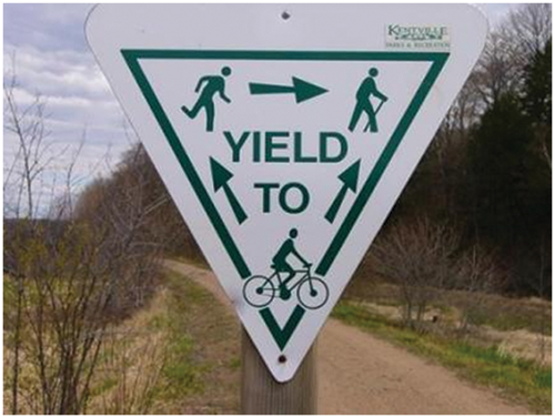
Figure 2: Method 2 traffic control
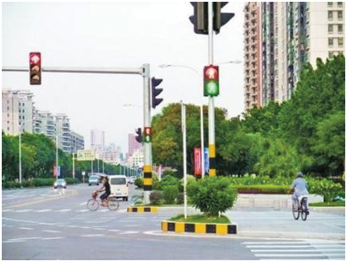
Figure 3: Method 3 traffic control
In China, the most frequently used traffic control modes at intersections are “roundabout control”, “Yield or Stop signs control”, and “traffic signal control”, where they also belong to the above three control methods, respectively [18]. For the sake of convenience, these three kinds of control models are denoted by
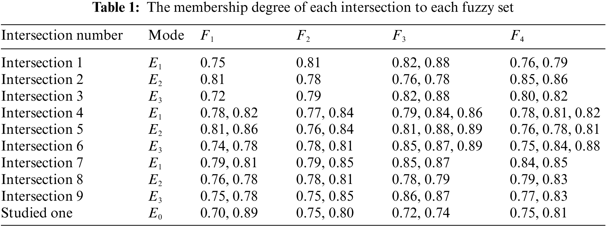
By information aggregation,
Similarly, the studied intersection could be expressed as a hesitant fuzzy set
In this subsection, the decision making problem is solved by using the novel distance measures. Firstly, sort the elements of each
Thereafter, for every
Then, the intervals corresponding to
The following, by
Analogously,
For
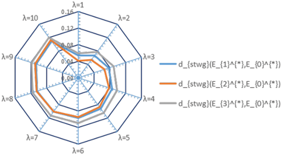
Figure 4: Distances obtained by using d__{stwg}
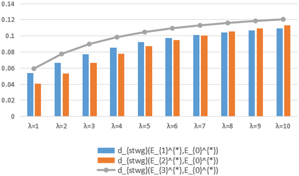
Figure 5: Contrast map of three kinds of distances
Figs. 4 and 5 illustrate that the suitable intersection Traffic Control mode varies as the parameter
In this subsection, the given problem can is solved by using classical methods. For example, by using Definition (3) proposed by Xu et al. [4], E0 can be transferred as
Then, for
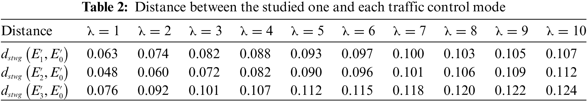
Table 2 illustrates that the suitable intersection traffic control mode varies as the parameter. Specifically, when
In calculating the distance between two HFEs with different cardinal numbers, the cardinalities of them should be unified. To reduce the uncertainty in the unifying process, equal-probability transformation is used. Specially, a series of improved distance measures on HFSs are proposed. Since the essence of equal-probability transformation is a kind of dimensional transformation of the same information in the way of expression, the proposed method retains the decision information completely. By contrast, it is difficult to achieve this effect using classical methods. Moreover, the main innovations of this study are concluded as follows:
(i) The theoretical basis of this study is to deal with the membership function value of HFSs from the viewpoint of probability. Moreover, an equal-probability transformation technique is proposed to transform any given HFE into a new one with specified cardinal number.
(ii) To express the enhancement effect for the same membership function value of HFE occurring more than once, impulse function is introduced into hesitant fuzzy fields. This is consistent with people’s production experience.
(iii) This study is a multidisciplinary combination of the theories of the cardinality, equal-probability mapping, and impulse function.
In general, the innovation of this study mainly lies in the unification of multi-source heterogeneous data. This innovation can be applied not only to HFSs, but also to HFSs or NFSs, etc.
Ethical Approval: This article does not contain any studies with human participants performed by any of the authors.
Funding Statement: The Fangwei Zhang’s work is partially supported by Shanghai Pujiang Program (No. 2019PJC062), the Natural Science Foundation of Shandong Province (No. ZR2021MG003), the Research Project on Undergraduate Teaching Reform of Higher Education in Shandong Province (No. Z2021046).
Conflicts of Interest: The authors declare that they have no conflicts of interest to report regarding the present study.
References
1. Zadeh, L. A. (1996). Fuzzy sets, fuzzy logic, and fuzzy systems, selected papers by Lotfi A. Zadeh. Singapore: World Scientific Publishing Company. [Google Scholar]
2. Torra, V. (2010). Hesitant fuzzy sets. International Journal of Intelligent Systems, 25(6), 529–539. DOI 10.1002/int.20418. [Google Scholar] [CrossRef]
3. Torra, V., Narukawa, Y. (2009). On hesitant fuzzy sets and decision. The 18th IEEE International Conference on Fuzzy Systems, pp. 1378–1382. Jeju Island, Korea. [Google Scholar]
4. Xu, Z. S., Xia, M. M. (2011). Distance and similarity measures for hesitant fuzzy sets. Inform Sciences, 181(11), 2128–2138. DOI 10.1016/j.ins.2011.01.028. [Google Scholar] [CrossRef]
5. Zhang, N., Wei, G. W. (2013). Extension of VIKOR method for decision making problem based on hesitant fuzzy set. Applied Mathematical Modelling, 37(7), 4938–4947. DOI 10.1016/j.apm.2012.10.002. [Google Scholar] [CrossRef]
6. Peng, D. H., Gao, C. Y., Gao, Z. F. (2013). Generalized hesitant fuzzy synergetic weighted distance measures and their application to multiple criteria decision-making. Applied Mathematical Modelling, 37(8), 5837–5850. DOI 10.1016/j.apm.2012.11.016. [Google Scholar] [CrossRef]
7. Rodríguez, R. M., Martínez, L., Torra, V., Xu, Z., Herrera, F. (2014). Hesitant fuzzy sets, state of the art and future directions. International Journal of Intelligent Systems, 29(6), 495–524. DOI 10.1002/int.21654. [Google Scholar] [CrossRef]
8. Sharp, H. (1968). Cardinality of finite topologies. Journal of Combinatorial Theory, 5(1), 82–86. DOI 10.1016/S0021-9800(68)80031-6. [Google Scholar] [CrossRef]
9. Dubois, D., Prade, H. (1985). Fuzzy cardinality and the modeling of imprecise quantification. Fuzzy Sets and Systems, 16(3), 199–230. DOI 10.1016/0165-0114(85)90025-9. [Google Scholar] [CrossRef]
10. Rosenblueth, E. (1975). Point estimates for probability moments. Proceedings of the National Academy of Sciences, 72(10), 3812–3814. DOI 10.1073/pnas.72.10.3812. [Google Scholar] [CrossRef]
11. Brownlee, K. A. (1965). Statistical theory and methodology in science and engineering. New York: Wiley. [Google Scholar]
12. Fan, C., Chen, J., Hu, K., Fan, E., Wang, X. (2022). Research on normal pythagorean neutrosophic set choquet integral operator and its application. Computer Modeling in Engineering & Sciences, 131(1), 477–491. DOI 10.32604/cmes.2022.019159. [Google Scholar] [CrossRef]
13. Liu, X. D., Wang, Z. W., Zhang, S. T., Garg, H. (2021). Novel correlation coefficient between hesitant fuzzy sets with application to medical diagnosis. Expert Systems with Applications, 2021. DOI 10.1016/j.eswa.2021.115393. [Google Scholar] [CrossRef]
14. Liu, X., Wang, Z., Zhang, S., Garg, H. (2021). An approach to probabilistic hesitant fuzzy risky multi-attribute decision making with unknown probability information. International Journal of Intelligent Systems, 36(10), 5714–5740. DOI 10.1002/int.22527. [Google Scholar] [CrossRef]
15. Mahmood, T., Ali, W., Ali, Z., Chinram, R. (2021). Power aggregation operators and similarity measures based on improved intuitionistic hesitant fuzzy sets and their applications to multiple attribute decision making. Computer Modeling in Engineering & Sciences, 126(3), 1165–1187. DOI 10.32604/cmes.2021.014393. [Google Scholar] [CrossRef]
16. Xia, M. M., Xu, Z. S., Chen, N. (2013). Some hesitant fuzzy aggregation operators with their application in group decision making. Group Decision and Negotiation, 22(2), 259–279. DOI 10.1007/s10726-011-9261-7. [Google Scholar] [CrossRef]
17. Roess, R. P., Prassas, E., McShane, W. R. (2011). Traffic engineering. 4th edition. New Jersey: Pearson Prentice Hall. [Google Scholar]
18. Wang, W., Guo, X. C. (2000). Traffic engineering. 4th edition. Nanjing, China: Southeast University Press. [Google Scholar]
19. Ministry of Housing and Urban-Rural Development of the People’s Republic of China (2010). Code for planning of intersections on urban roads. Beijing: Standards Press of China. [Google Scholar]
20. Ministry of Construction of the People’s Republic of China (1995). Code for transport planning on urban road. Beijing, China: Standards Press of China. [Google Scholar]
21. Ministry of Housing and Urban-Rural Development of the People’s Republic of China (2006). Code for design of urban road engineering. Beijing: Standards Press of China. [Google Scholar]
22. Zhang, F. W. (2016). Several kinds of uncertain multi-attribute decision-making methods and their application in transportation management. Beijing, China: People’s Communication Press. [Google Scholar]
23. Goldberg, D. (1991). What every computer scientist should know about floating-point arithmetic. ACM Computing Surveys, 23(1), 5–48. DOI 10.1145/103162.103163. [Google Scholar] [CrossRef]
Cite This Article
 Copyright © 2023 The Author(s). Published by Tech Science Press.
This work is licensed under a Creative Commons Attribution 4.0 International License , which permits unrestricted use, distribution, and reproduction in any medium, provided the original work is properly cited.
 Downloads
 Citation Tools