AWK-TIS: An Improved AK-IS Based on Whale Optimization Algorithm and Truncated Importance Sampling for Reliability Analysis

Nomenclature

1  Introduction

Structural reliability analysis is often carried out to quantitatively assess the probability of structures’ safe or failure state under the impact of uncertain factors in the environmental, structural and load parameters. Various structural reliability analysis methods, which can be broadly categorized into three main types: simulation-based methods, analytical methods or approximation methods, and meta-modeling methods, have been proposed over the past three decades [1,2].

Concerning simulation-based methods, the crude Monte Carlo simulation (MCS) method is the basic form of this classification, which evaluates the failure probability by dividing the number of samples falling into the failure domain by all the samples generated from the limit state evaluations. Although MCS is the most convenient implementation approach, it is extremely time-consuming when dealing with small failure probability and complex numerical models (e.g., fidelity finite element models (FEM)). Meanwhile, tremendous variation techniques of the MCS such as subset simulation [3,4], importance sampling [5,6] and directional sampling [7,8] have been developed to obtain more accurate results with fewer samplings. However, the main drawback of insufficient still exists in those methods.

As analytical methods, the traditional first-order and the second-order reliability methods (FORM and SORM) [9–12] respectively approximate the limit state function (LSF) around the most probable failure point (MPP) with first-order and incomplete second-order functions. The derivatives of the LSF with respect to the random variables have thus to be evaluated. Hence, these methods are not suitable for implicit limit state function and high nonlinearity cases.

Meta-modeling methods have been developed to balance the computational accuracy and efficiency during the structural reliability analysis, such as response surfaces [13–15], polynomial chaos expansion [16,17], artificial neural networks [18,19], support vector machine [20,21], radial basis function (RBF) [22,23] and Kriging metamodel [24,25]. In recent years, Kriging metamodel methods have obtained remarkable attention in the state-of-the-art literature. From the design of experiment (DOE) aspect of view, the strategy for constructing a Kriging model can broadly be classified into two sorts, the one is “one-shot” and the other is adaptive sampling or sequential sampling methods [26]. Literally, “one-shot” means producing enough design points before generating a Kriging model without supplementing new sample points in succeeding courses. Nevertheless, the adaptive sampling methods generate a relatively small number of design points at the initial step, and then add one or more samples in each course of iteration according to certain regulations [27]. Furthermore, the exclusive feature of Kriging that it can predict the local uncertainty along with the prediction value promotes the development of the adaptive Kriging [24,28].

Two typical algorithms, the efficient global reliability analysis (EGRA) [28] and adaptive Kriging (AK) with MCS (AK-MCS) [29], are generously adopted and depict outstanding characters in diverse structural reliability problems. The amount of research has then further ameliorated the performance of active Kriging-based methods in recent years. These ameliorations resort to different and more efficient learning functions, sampling schemes and stopping criteria. Learning functions include the expected feasible function (EFF) [28], the learning function U [29], the learning function H [30], expected risk function (ERF) [31], least improvement function (LIF) [32], reliability-based expected improvement function (REIF) [33], Folded Normal based Expected Improvement Function (FNEIF) [34], K-means and weighted K-medoids algorithms-assisted learning process [35], and PDEM-oriented expected improvement function (PEIF) [36]. With regard to stopping criteria, it is common to see that when the values of learning functions reach certain thresholds the learning process stopped. For sampling tactics, importance sampling, subset simulation, line sampling, etc. have been adopted to evaluate failure probability in active Kriging (AK) reliability analysis, and some AK-based sampling methods were presented, such as AK-IS [37], AK-SS [38], AK-DS [39], AKOIS [40], AK-ARBIS [41], AK-SESC [42] and AKSE [43]. By combining these sampling methods with learning functions, the number of calls of limit state functions has reduced dramatically with acceptable accuracy of variation coefficient of failure probability. Despite the aforementioned learning functions, the correlation parameter θ also plays a vital role in constructing an accurate Kriging model. Thus, the pattern search algorithm is applied in DACE to calculate the optimum of θ [44]. However, as a local optimization algorithm, pattern search is sensitive to the initial value and may get trapped in local optimum. Then, various global optimization algorithms, such as genetic algorithm (GA) [33,45], DIRECT algorithm [46], particle swarm optimization (PSO) [47], and artificial bee colony (ABC) [48], are adopted to find the optimal value of θ by solving the maximum likelihood equation. Compared with GA, PSO, and the pattern search, the whale optimization algorithm (WOA) [49] proposed in the year of 2016 has its own advantages, such as simple principle, easy implementation, high convergence speed and calculation accuracy.

This paper aims to improve the efficiency and accuracy of the AK-IS for structural reliability analysis. In this paper, AWK-TIS is proposed, which is inspired by AK-IS [34] and RBF-GA [50], coupling with WOA and Truncated importance sampling (TIS) [51,52], and the WOA in AWK-TIS is adopted to seek the optimum of correlation parameter θ and the MPP in different phases of each course of iterations. Moreover, inside of the optimal β-sphere treated as the safe state, the samples are eliminated by TIS. Therefore, the prediction of Kriging model and the selection of the best next sample are only implemented through the candidate samples outside the optimal β-sphere, which significantly reduces the computational time and saves computer memory in comparison with the original AK-IS.

The remainder of the manuscript is organized as follows. Section 2 briefly introduces the Kriging method, AK-IS method, TIS and WOA. In Section 3, the procedures and the main steps of the AWK-TIS method are proposed. In Section 4, the applicability of the proposed technique is validated by four numerical cases and one real engineering problem of jet van manipulation mechanism. Finally, conclusions are summarized in Section 5.

2  Backgrounds

Before introducing the proposed AWK-TIS algorithm, some basic theories are briefly recalled, e.g., the Kriging method, the main steps of the AK-IS algorithm and truncated importance sampling (TIS) method, and the WOA.

2.1 Basic Theory about Kriging Method

Kriging metamodel, which consists of a parametric linear regression model and a nonparametric stochastic process, is an interpolation technique based on statistical theory. It needs a DOEs to determine its stochastic parameters and then predictions of the response can be inferred on any unknown point. Give a set of initial DOEs X = [x1, x2, …, xm], with xiϵRn(i = 1, 2, …, m) the ith experiment, and G = [G(x1), G(x2), …, G(xm)] is the corresponding response to X. The approximate relationship between any experiment x and the response G(x) can be denoted as [41,42]:

G^(x)=F(ξ,x)+z(x)=fT(x)ξ+z(x)(1)

where ξT=[ξ1,…,ξp] is a regression coefficient vector, fT(x)=[f1(x),f1(x),…,fp(x)]T is the basic functions vector which makes a global simulation in design space. In the ordinary Kriging, F(ξ,x) is a scalar and always taken as F(ξ,x)=ξ;z(x) is a stationary Gaussian process with zero mean and covariance between two data points xi and xj is denoted as:

Cov[z(xi),z(xj)]=σz2R(xi,xj)(2)

where σz2 is the process variance, and xi,xj are data points from the whole samples X.R(xi,xj) is the correlation function about xiandxj with a correlation parameter vector θ that has to be estimated by pattern search method in DACE. A diversity of models can be adopted to define correlation function R(xi,xj), such as Gaussian correlative model, experimental and linear model, etc. The widely employed Gaussian model is accepted in the paper and can be defined as:

R(xi,xj)=exp∑k=1n[ −θk(xik−xjk)2 ] θk≥0 (3)

where n is the dimension of the sample, xik,xjk and θk are the kth components of data sample xi,xjandθ, respectively.

Define correlation matrix R=[R(xi,xj)]m×m, F is a m × 1 unit vector, then ξ and σz2 are given by:

ξ^=(FTR−1F)−1FTR−1G(4)

σ^z2=(G−ξ^F)TR−1(G−ξ^F)/m(5)

where R, ξ^ and σ^z2 are functions of θ.

Then at an unknown point x, the Best Linear Unbiased Predictor (BLUP) of the response G^(x) is shown to be a Gaussian random variant G^(x)∼N(μG^(x),σG^(x)), where

μG^(x)=ξ^+r(x)R−1(G−ξ^F)(6)

σG^2(x)=σz2(x)(1+vT(x)(FTR−1F)−1v(x)−rT(x)R−1r(x))(7)

where r(x)=[R(x,x1),R(x,x2),…,R(x,xm)], v(x)=FTR−1r(x)−1. μG^(x) is usually taken as the estimated G^(x) at point x. That means Kriging is an exact interpolation method.

The correlation parameter θ can be obtained through the maximum likelihood estimation (MLE) [47,48]:

θ=argminφ(θ)=argmin(mln⁡σ^z2+ln⁡|R|)(8)

where |R| is the determinant of R. The optimal Kriging model can be obtained if the optimal correlation parameter θ∗ is guaranteed. The Eq. (8) can be solved by pattern search method, genetic algorithm, PSO, etc. It should be noted that since the introduction of WOA, this algorithm has been used in many fields and showed its superiority over many other metaheuristic algorithms such as PSO, ABC, GA, etc. As a result, WOA is adopted to search θ∗ in this study.

2.2 AK-IS Algorithm

AK-IS mainly consists of two steps. The first step is the FORM approximation, which is utilized to find the MPP that is not accurate enough to evaluate the probability. The second step is to establish an AK model with a special learning function and stopping criteria to reduce the calls of original limit state function. In this step, IS method is adopted to calculate the failure probability and its coefficient of variation.

IS requires the definition of a joint PDF φn that is taken as a standard Gausssian one centered at the MPP found in the first step for the new sampling. The failure probability is estimated as [37]:

Pf=∫RnIF(u)ϕn(u)φn(u)φn(u)du1⋯dun(9)

where IF(u) is indicator function, IF(u))={0ifG(u)>0and1ifG(u)≤0}.

A number of NIS samples denoted {u~(i), i = 1, …, NIS} are generated according to importance sampling density function φn. The integral is then expressed by:

Pf≈P^f,IS=1NIS∑i=1NISIF(u~(i))ϕn(u~(i))φn(u~(i))(10)

The variance of the failure probability estimator is given as:

Var[P^f,IS]=1NIS(1NIS∑i=1NIS(IF(u~(i))(ϕn(u~(i))φn(u~(i)))2)−P^f,IS2)(11)

The coefficient of variation δIS of the failure probability estimator is then:

δIS=Var[P^f,IS]P^f,IS(12)

Besides, the learning function U proposed in AK-MCS is still used in AK-IS:

U(x)=|μG^(x)|σG^(x)(13)

where μG^(x) and σG^(x) are Kriging mean and standard deviation, respectively. Moreover, the sample that has the minimum of U(x) is called the best next sample and it is iteratively enriched the DOE to update the Kriging model. The learning process stops if the minimum of the learning function U is larger than its threshold. Besides, the active procedure continues and NIS new samples are enlarged until the coefficient of variation δIS is smaller than a limit value which is set to 0.05 in AK-IS.

2.3 Truncated Importance Sampling

Truncated importance sampling (TIS) method is developed by introducing a hypersphere with the radial, which is indicated by β shown in Fig. 1, equals to the minimum distance from the origin to the limit state surface in u-space [51,52].

Figure 1: Sketch of TIS

The red point in Fig. 1 indicates the MPP.

The indicator function of the outer of the β-sphere is defined as follows:

Iβ(u˜(i))={ 0if| | u˜(i) | |2≤β21if| | u˜(i) | |2>β2(14)

where the inner of the β-sphere contains part of the safe domain or even all of the district, while other domains including all the failure domain and part of the safe domain are out of the β-sphere. It can be seen that the indicator function IF of the samples located in the β-sphere is IF(u~)=0, and there is unnecessary to call the true model to evaluate whether safe or not. The integral is then estimated by:

Pf≈P^f,TIS=1NIS∑i=1NISIF(u~(i))Iβ(u~(i))ϕn(u~(i))φn(u~(i))(15)

The variance of the failure probability estimator is estimated as:

Var[P^f,TIS]=1NIS−1(1NIS∑i=1NIS(IF(u~(i))Iβ(u~(i))(ϕn(u~(i))φn(u~(i)))2)−P^f,TIS2)(16)

The coefficient of variation (C.O.V) δTIS of the failure probability estimator is then:

δTIS=Var[P^f,TIS]P^f,TIS(17)

2.4 Whale Optimization Algorithm

The Whale Optimization Algorithm (WOA) is a novel nature-inspired population-based meta-heuristic algorithm, presented by Seyedali Mirjalili and Andrew Lewis from Griffith University in 2016 [49]. It was abstracted from the special hunting behavior of humpback whales. This foraging behavior is named bubble-net feeding method.

Two approaches namely, shrinking encircling mechanism and spiral updating position, are designed to mathematically model the exploitation phase of the WOA. The first approach is formulated as follows:

xi(t+1)=xbest(t)−Ai⋅|Ci⋅xbest(t)−xi(t)|(18)

where t indicates the current iteration, Ai and Ci are coefficients. xi(t) and xbest(t) represent i-th search agent and the best agent in the t-th iteration, respectively.

Ai=2q⋅ri1−q(19)

Ci=2ri2(20)

where q is linearly reduced from 2 to 0 over the course of iterations, ri1, ri2 are random numbers in [0, 1]. Ai is a random value in the interval [−2q, 2q]. When the random value of Ai is in [−1, 1], the next position of a search agent can be in any position of the agent and the position of the current best agent. The parameter Ci is a random value in [0, 2]. This component provides random weights for prey in order to stochastically emphasize (Ci > 1) or deemphasize (Ci < 1) the effect of prey in defining the distance between the search agent and the current best agent. Besides, the second approach, the process of spiral updating position, is expressed as follows:

xi(t+1)=xbest(t)+|xbest(t)−xi(t)|⋅ebl⋅cos⁡(2πl)(21)

where b is a constant for defining the ‘9’-shaped path of distinctive bubbles created by the humpback whales, l is a random number in [−1, 1].

The humpback whales hunt the prey by using the shrinking circle mechanism and spiral updating method simultaneously, and the two approaches have the same possibility to be chosen, so the model of the exploitation phase is as follows:

xi(t+1)={ xbest(t)−Ai⋅| Ci⋅xbest(t)−xi(t) | if ri3<0.5xbest(t)+| xbest(t)−xi(t) |⋅ebl⋅cos(2πl) if ri3≥0.5(22)

where ri3 are random numbers in [0, 1] to switch the different mathematical model of exploitation.

However, the process of search for prey is defined as the exploration phase, and the model of this phase is described as follows:

xi(t+1)=xj(t)−Ai⋅|Ci⋅xj(t)−xi(t)|(23)

where xj(t) is the j-th random search agent which is different from the xi(t), and Ai is also defined by Eq. (19), but it is absolute value, |Ai|, is greater than 1 to emphasize exploration and let the WOA to search the whole search space.

3  AWK-TIS Algorithm

In this section, the main steps of the proposed method are introduced. Firstly, the WOA-Kriging model is constructed based on the basic Kriging model. Secondly, the AWK-TIS method is developed.

3.1 WOA-Kriging Model

In the proposed WOA-Kriging model, the optimal value of correlation parameter θ* is calculated by integrating WOA into the basic Kriging model. The pattern search method is adopted to seek θ* in DACE. However, the pattern search method is a local optimization algorithm that needs an initial solution to search the optimal and it is easy to get trapped in the local optimum. Alternatively, while seeking θ*, as an efficient global optimization algorithm not depend on the initial solution. WOA is embedded in the DACE toolbox to solve Eq. (8), instead of pattern search algorithm. Then, in our implementations the fitness function for the MLE according to the correlation parameter θ is to minimize the function below [45]:

Minimize: ϕ(θ)=|R|1/mσ^z2Subject to:θk>0,k=1,2,…,n(24)

Given the fitness function above, the finding process of θ* becomes a typical minimization problem. Thus, the population (whale positions) is firstly initialized in a n-dimensional search space, and the population size is set to 25 in this study. Each position corresponds to a correlation parameter vector. Next, a set of mathematical rules in WOA such as encircling prey, spiral bubble-net feeding and search for prey are repeatedly conducted at each iteration. Then, the fitness values of every population are obtained, the fittest solution is ascertained. Finally, the global optimal correlation parameter is acquired until the satisfaction of the stopping criteria that is the maximum number of iterations equals to 100. The main WOA parameters are unchanged during the optimization procedure. Consequently, the WOA-Kriging model is constructed by the optimal correlation parameter θ*.

3.2 The AWK-TIS Algorithm

In this subsection, the AWK-TIS algorithm is introduced in detail. In AWK-TIS, the real limit state function is substituted by a WOA-Kriging model; the failure probability and its coefficient of variation are computed by TIS method in an active learning way. AWK-TIS mainly consists of three components. Firstly, a WOA-Kriging model is constructed according to the optimal parameter θ* searched by WOA and the DOE generated through Latin Hypercube Sampling method in the entire design space. Secondly, MPP is evaluated by WOA and the evaluation process is treated as solving a constrained optimization. Thirdly, the active learning method and TIS are adopted together to conduct the selection of the best next sample and the evaluation of the probability. At this stage, the WOA-Kriging model is updated according to the enriched DOE. The general sketch of the AWK-TIS is shown in Fig. 2, and the detailed procedure is proposed as follows:

Step 1: Generation of the initial DOE. Latin Hypercube Sampling (LHS) method is employed to generate the initial samples in the whole design space. Then, the structural response or the real limit state function of every initial sample is evaluated. Thus, the initial DOE is composed of the initial samples and their corresponding responses. The number of the initial samples has an effect on the accuracy of the WOA-Kriging model; however, there are no certain rules to certificate this number.

Step 2: Construction of the WOA-Kriging model. Construct the WOA-Kriging based on initial DOE by embedding WOA to DACE toolbox to find the optimal parameter θ*. Calculating θ* will spend a little more computing time, but it is worth since the time consumed for finding accurate parameters could be ignored compared with that for time-consuming simulations. The initial value of θ is unnecessary in this metamodel construction, and the correlation function is chosen to be the Gaussian function.

Step 3: Evaluation of the MPP. The WOA is utilized to calculate the MPP. The notion of reliability index β, is the minimum distance from the origin to the limit state surface in the standard normal space. The reliability index can be therefore calculated as the following constrained optimization problem [9,47,48]:

Minimize:β=min∑i=1n(xi∗)2=min∑i=1n[(xi−μxi)/σxi]2Subject to:G^(x)=0(25)

where x denotes the vector of random variants, which is x=(x1,x2,…,xn);xi∗ denotes the standard normal variants; μxi and σxi represent the mean and standard deviation of the random variant xi, respectively. G^(x) is the limit state function constructed by WOA-Kriging model.

Figure 2: General sketch of the AWK-TIS algorithm

The problem in Eq. (25) is a constrained nonlinear optimization problem. The aim of constraint optimization is to search for feasible solutions with better objective values. However, constrained optimization problems are difficult to solve than unconstrained optimization problems due to the presence of constraints and their interrelationship between the objective functions. As a result, the main assignment while solving the constrained optimization problem is to deal with the constraints.

Step 3.1: Construction of unconstrained function

To avoid the violation of constraints, unfeasible solutions should be adapted to feasible solutions. In the meta-heuristic community, the most common technique is to take advantage of penalty functions to handle these constraints. Thus, a penalty function is employed to convert the constrained optimization problem in Eq. (25) to the unconstrained one in Eq. (26) [21]:

β=minF(x∗)=min∑i=1n(xi∗)2+λG^(x)2(26)

where, λ is the positive penalty coefficient, and its initial value is set to 103 in this paper.

Step 3.2: Calculation of reliability index by WOA

The WOA is adopted to solve the unconstrained function. The inner loop is to find the optimal solution of the Eq. (26) by WOA, while the outer loop is to make sure that the reliability index β is accurate enough. Thus, two stop criteria should be satisfied simultaneously as follows. First, the relative error between the reliability indices in two subsequent outer loop iterations is acceptable [47]:

|βk+1−βk|/βk<ζ(27)

where k and k + 1 indicate the k-th and k + 1-th iteration in the outer loop, respectively, and relative error ζ is a small constant (e.g., 0.01).

Second, it is required that the value of the WOA-Kriging model at the “potential” MPP should be relatively small which means that the “potential” MPP is rather close to the LSF [48]:

λG^(x)2≤χ(28)

where χ is the threshold which is also a small constant (e.g., 0.0001).

If the two criteria above are met simultaneously, the MPP is acquired; otherwise, let λ = 10λ and go back to Step 3.1. It is noted that in this step the parameters in WOA are remain the same as its original version.

Step 4: Generation of NIS samples. NIS samples are generated according to importance sampling density function centered on the MPP found by Step 3. The response of those samples will be evaluated by WOA-Kriging if the active learning procedure requires it.

Step 5: Conduction of the active learning procedure. Add {xu, G(xu)} into the DOE set to rebuild the WOA-Kriging model, and evaluate the learning function U among NIS samples. The learning process continues until the stop criterion, i.e., min(U(xi)) > 2 is satisfied, which means that the probability of making wrong sign estimation should not exceed 2.3%.

Step 6: Evaluation of the failure probability and the coefficient of variation δTIS. After the WOA-Kriging metamodel is constructed by the active learning method, the next step is to adopt TIS to analyze the reliability. The failure probability and the coefficient of variation are estimated δTIS by Eqs. (15) and (17), respectively, and make sure that the δTIS satisfies the predefined threshold. If δTIS does not satisfy the threshold, a set of new NIS samples are generated to enrich the original NIS samples. In this paper, the threshold of the δTIS is taken as 0.05.

Step 7: Output the unbiased estimation of the failure probability. If δTIS satisfies the threshold, i.e., δTIS ≤ 0.05 then AWK-TIS terminates, and the failure probability is acquired.

4  Validation Cases

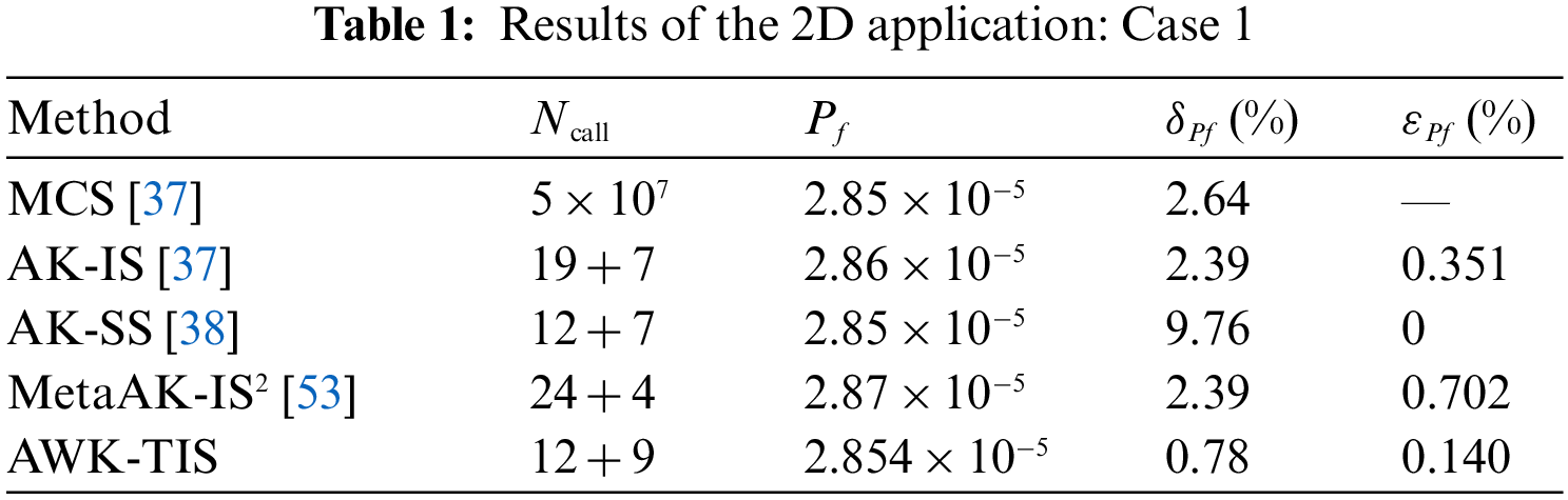
In this section, the efficiency of AWK-TIS is illustrated by four numerical cases and one engineering case. Each of the cases in this study has only a single failure region, which means only one MPP in each case. All the case results are averaged over 10 different runs. The accuracy and efficiency of different algorithms is compared according to the number of calls to the LSF (Ncall), δPf (the coefficient of variation of failure probability) and εPf (the relative percentage error of failure probability in comparison with the reference value).

4.1 Case 1: 2D Application

A 2D numerical case, which has two independent random variables with standard normal distribution, is chosen to illustrate the process of the proposed method. The limit state function reads

G(u)=0.5(u1−2)2−1.5(u2−5)3−3(29)

In the proposed method, an initial Kriging model is constructed based on 12 samples within the domain of [±6] in u space. The results of different methods are summarized in Table 1. The proposed method AWK-TIS is compared with AK-IS, MetaAK-IS2, AK-SS. The reference value evaluated by MCS with 5 × 107 samples is taken from [37], and the value is 2.85 × 10−5. In order to test the robustness of AWK-TIS, 10 different runs are performed with NIS = 1 × 105 initial samples centered on the MPP confirmed by WOA. According to Ncall, i.e., the number of calls to the LSF, the proposed AWK-TIS outperforms the majority of active learning Kriging-based methods except for AK-SS; however, the δPf, i.e., the coefficient of variation of failure probability of AK-SS is higher than that of AWK-TIS.

Furtherly, the approximation process of the limit state function is schematically illustrated in Fig. 3, including LSF (green line), Kriging model (red dotted line), initial samples (black fork dots), added samples (pink circle) and MPP (blue hexagon). Moreover, the MPP searched by WOA is located almost in the same position after 5 iterations while the enriched DOE are updated sequentially by U learning function. The convergence process of failure probability Pf and the C.O.V of Pf for AWK-TIS are presented in Fig. 4.

Figure 3: The approximation process of the LSF for case 1

Figure 4: Convergence process of Pf and C.O.V of Pf for case 1

It can be seen from Figs. 3 and 4 that these newly computed samples are located in the vicinity of the limit state function and are used to improve the accuracy of Kriging metamodel. Moreover,AWK-TIS requires much less performance function computations than AK-IS. Indeed, AWK-TIS needs 9 computations of real limit state function after the construction of Kriging model by initial DOE.

As described in Section 2.4, the WOA is adopted to acquire the correlation parameter θ. The number of search agents is 25, the number of iterations is set to 100, and other parameters in WOA are remaining as the original form. Fig. 5 depicts the convergence of the Kriging correlation parameter θ shown in Eq. (8) when the update process of the WOA-Kriging model is stopped. Moreover, Fig. 5 shows that the maximum likelihood estimation of θ convergence to the minimum value of 6.49 × 10−6 at the 16th iteration, and the optimum θ is found at this point. Compared with PSO and GA, the WOA shows its high convergence speed and calculation accuracy.

Figure 5: The process to find θ* using WOA for case 1

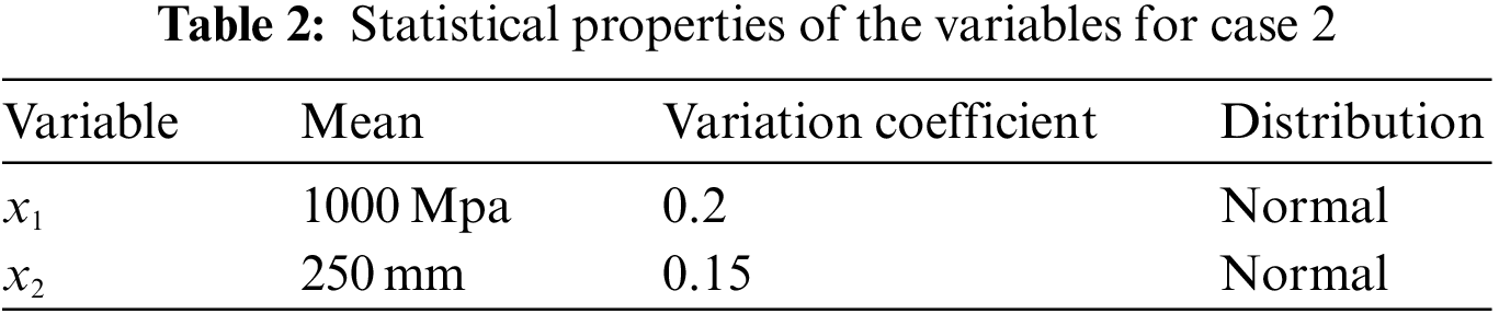
4.2 Case 2: A Cantilever Beam Example

This case has been widely used in literature [38]. The cantilever beam, which has a rectangular cross-section, is subjected to a distributed uniform load. The limit state function which is defined by the maximum vertical displacement of the beam is given as

G(x)=0.01846154−74.76923x1/x23(30)

where x1 and x2 are assumed to be independent random variables following normal distribution. The statistical properties of the above two variables are shown in Table 2. The results obtained by the proposed AWK-TIS, MSC, AK-MCS, and AK-SS are listed in Table 3.

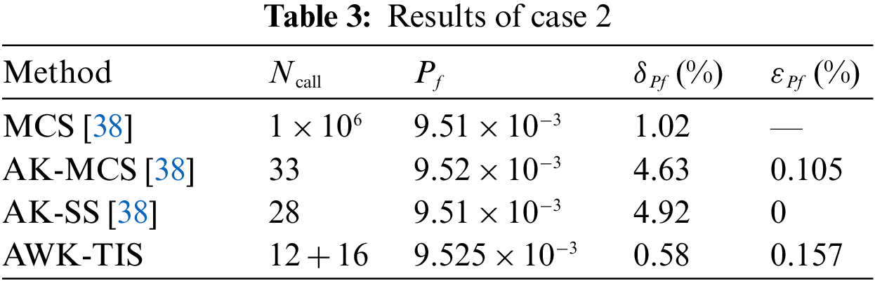
From Table 3, it can be seen that the Ncall of the proposed AWK-TIS is the same as that of AK-SS, but it is less than the number of samples applied in AK-MCS. Besides, the one can see that all the Pf calculated by the different methods have high accuracy comparing with the MCS solution. However, the coefficient of variation of failure probability of AWK-TIS is the smallest in the four methods.

Similarly to Figs. 3 and 4, Fig. 6 shows the final approximation of AWK-TIS and Fig. 7 shows the convergence process of failure probability and the C.O.V of failure probability. As shown in Fig. 6, the added samples are almost in the vicinity of the real LSF, and the LSF constructed by Kriging can be accurately approximated in the domain of the sampling region. On the contrary, the Kriging model shows inexact outside the sampling region. Nevertheless, it should be indicated that the region outside the sampling area has little influence on the failure probability calculation due to the MPP is far away from this area. From Fig. 7, the proposed method has converged to the final results at about 12 added samples, which indicates the efficiency and accuracy of the AWK-TIS.

Figure 6: The approximation of the LSF for case 2

Figure 7: Convergence process of Pf and C.O.V of Pf for case 2

4.3 Case 3: A Non-Linear Oscillator

A non-linear undamped single degree of freedom system depicted in Fig. 8 is analyzed in this case. The limit state function is given as [54]

G(C1,C2,M,R,T1,F1)=3R−|2F1Mω02sin⁡(ω0T12)|(31)

where ω0=(C1+C2)/M. Six random input variables including C1, C2, M, R, T1, and F1 are listed in Table 4. The initial number of DOE is set as 20. The AWK-TIS is compared with several other existing methods (MCS, AK-MCS, PAK-Bn [54]) and their results are listed in Table 5. Same as the two cases above, the reference values to compare the reliability analysis results are the Pf,, C.O.V of Pf, δPf, εPf, estimated by MCS.

Figure 8: A non-linear oscillator

It can be seen from Table 5 that although the relative error of failure probability obtained by the proposed method is slightly larger than that of AK-MCS and PAK-Bn, the Ncall of AWK-TIS is significantly reduced contrasted with that of the two methods above. Additionally, the C.O.V of failure probability is rather small compared with the other three methods. Hence, it indicates that AWK-TIS could solve the problem of small failure probability with a moderate number of random variables.

Equally, Fig. 9 presents the convergence process of failure probability and C.O.V of failure probability of this case. From Fig. 9, one can see that the failure probability has converged with almost 50 added samples, which means that the proposed AWK-TIS is suitable for the calculation of the small failure probability.

Figure 9: Convergence process of Pf and C.O.V of Pf for case 3

4.4 Case 4: A Roof Truss Structure

A roof truss structure, which is selected to verify the proposed method, is shown in Fig. 10. The roof truss undertaking the uniformly distributed load q that can be converted to the nodal load P = ql/4. The response of the roof truss is the perpendicular deflection △C of node C is denoted as [55]:

ΔC=ql22(3.81ACEC+1.13ASES)(32)

where AC, AS, EC, ES respectively are sectional area, elastic modulus concrete and steel bars, l is the length of the structure. The mean and variation coefficient of the six independent normal distribution random variables are reported in Table 6. The threshold of △C should not be larger than 0.03 m, and the LSF of this case is thus defined as

G(x)=0.03−ΔC(33)

Figure 10: The schematic diagram of a roof truss

The AWK-TIS is compared with other existing methods (MCS, AK-MCS, KAIS, RBF) and the results are summarized in Table 7. The results by MCS calculations with 1.06 × 106 samples are regarded as reference values in this case.

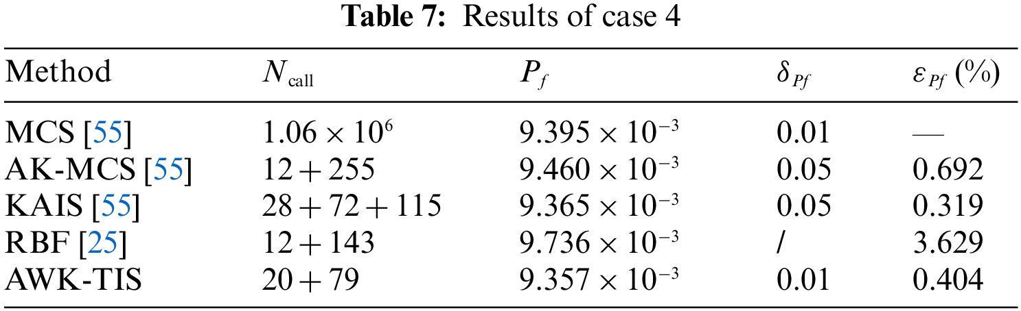
It can be seen from Table 7 that AWK-TIS needs only 99 Ncall to acquire a satisfactory result while the other three approaches demand more than 150 Ncall. The small Ncall has highlighted the numerical efficiency of the proposed approach in estimating the roof truss structure. Furthermore, the AWK-TIS has the second relative error of 0.404% comparing with the reference value of Pf evaluated by MCS, followed by AK-MCS and RBF.

By investigating the convergence process of Pf and C.O.V of Pf presented in Fig. 11, we can see that both of the curves converged at about 25 added samples, which means that the proposed AWK-TIS is suitable for dealing with small failure probabilities and relatively large number of random variables. Additionally, the convergence threshold can be advisably loosed to further improve computational efficiency.

Figure 11: Convergence process of Pf and C.O.V of Pf for case 4

4.5 Case 5: A Jet Vane Manipulation Mechanism

Vertical launch missile is widely used on land air defense and sea air defense. The performance of a jet vane system is extremely vital to the flying control of vertical launch missile. As a significant component of the jet van system, the manipulation mechanism drives the rudder rotating in the engine gas flow that generates pitch moment to control the orientation of the missile, which is shown in Fig. 12a. The manipulate mechanism convers the linear motion of the servo motor to the rotation of the jet van, and the schematic of this mechanism is shown in Fig. 12b.

Figure 12: A jet van manipulation mechanism

In Fig. 12b, A and B represent the positions of the two ends of the linkage respectively, and C is the center of the shaft. L1 and L2 are the length of linkage and rocker respectively. L3 is the distance between A and C along the X-axial. a is the distance between A and C. S is the maximum displacement of A along the negative direction of X-axial, and Al, Bl are the left limit position of the linkage. θ2 is the angle between the BC and the X-axial, and it is the function of L1, L2, L3, a and S, which is shown in Eq. (34)

θ2=π−arctan⁡(a−L1sin⁡θ1L3−S−L1cos⁡θ1)(34)

where θ1 is the angle between the linkage and the X-axial.

In this case, the linkage length L1, the length of the rocker L2, the distance between A and C along the X-axial L3, and the maximum displacement of linear servo system S are taken as random variables. Table 8 lists the details of random variables. To assure the normal operation of the manipulation mechanism, the maximum angle of the rudder shaft should not exceed a given threshold. Therefore, the limit state function is defined as

G(X)=θm−θ2(X)(35)

where θm is the threshold of the maximum angle of the rudder shaft which is taken as 118.2°, θ2(X) is the maximum angle of the rudder shaft which is calculated by solving Eq. (34), the X represents all the random variables.

The results of the different methods are shown in Table 9, in which results estimated by the AK-MCS and AK-IS methods are also provided for the sake of comparison. Besides, the calculation times or CPU-time of different AK-based algorithm are also exhibited in this table. The sample pool of the MCS, AK-MCS and AK-IS are 5 × 107, 5 × 106 and 4 × 106, respectively.

Table 9 shows that the predictive accuracy of the AWK-TIS notably outperforms the other two AK methods considering the relative error of failure probability. Besides, the Ncall is less than that of AK-MCS and AK-IS, which indicates that the proposed AWK-TIS can solve real engineering problem efficiently. From the CPU-time results, it is concluded that although the process of optimizing Kriging model by WOA algorithm additionally increases the computational time, the utilization of the TIS method reduces the calculation time.

The convergence of failure probability and coefficient of variation of failure probability is presented in Fig. 13. From Fig. 13, the Pf and C.O.V of Pf have converged to the final results at about the 10 added samples. Thus, the computational performance of the AWK-TIS when dealing with this case can be improved with a loose stopping criterion.

Figure 13: Convergence process of Pf and C.O.V of Pf for case 5

5  Conclusions

The AWK-TIS method is proposed as a novel reliability method to deal with structural reliability problems, in which the WOA is performed to seek the optimum correlation parameter of Kriging model and the MPP, and then the added samples generated by U learning function are enriched to DOE to refine the Kriging model. The MPP is calculated by WOA through solving the constrained nonlinear optimization problem until certain two thresholds are satisfied simultaneously. Afterward, the TIS method is applied to calculate the failure probability and coefficient of variation of the failure probability. In AWK-TIS, the sample pool is much smaller than that of AK-IS, which significantly expedites the learning efficiency. Five test cases including four numerical cases and one engineering case are adopted to verify the performance of the AWK-TIS method. Results prove that the proposed method can achieve high computational accuracy and efficiency.

AWK-TIS method has two main drawbacks: (1) AWK-TIS, like AK-IS, is dependent on the MPP to ensure the next best point; however, the solitary sampling center has confined its employment in dealing with multi-MPP problems, (2) the process of acquiring the MPP is transformed to solve the constrained nonlinear optimization problem, which may affect the efficiency of the proposed method, (3) due to the restriction of IS-based algorithm, the proposed algorithm does have some defects in dealing with high-dimensional problems. Future works will focus on three aspects: (1) adopt other efficient sampling methods in lieu of TIS to solve multi-MPP problems, (2) improve the efficiency of WOA by hybridising other optimizers or employing other more effective optimization algorithms to solve the constrained optimization problem to obtain the MPP, (3) alternative modeling and analysis methods need to be incorporated for effective validation of AWK-TIS to high-dimensional problems.

Funding Statement: This work is supported by the Technical Basic Scientific Research Projects of State Administration of Science, Technology and Industry for National Defence, PRC (Grant No. JSZL2019204C001).

Conflicts of Interest: The authors declare that they have no conflicts of interest to report regarding the present study.

References

1. Guimarães, H., Matos, J. C., Henriques, A. A. (2018). An innovative adaptive sparse response surface method for structural reliability analysis. Structural Safety, 73, 12–28. DOI 10.1016/j.strusafe.2018.02.001. [Google Scholar] [CrossRef]
2. Moustapha, M., Marelli, S., Sudret, B. (2022). Active learning for structural reliability: Survey, general framework and benchmark. Structural Safety, 96, 102174. DOI 10.1016/j.strusafe.2021.102174. [Google Scholar] [CrossRef]
3. Li, H. S., Cao, Z. J. (2016). Matlab codes of subset simulation for reliability analysis and structural optimization. Structural and Multidisciplinary Optimization, 54, 1–20. DOI 10.1007/s00158-016-1414-5. [Google Scholar] [CrossRef]
4. Zhang, J. H., Xiao, M., Gao, L. (2019). An active learning reliability method combining Kriging constructed with exploration and exploitation of failure region and subset simulation. Reliability Engineering and System Safety, 188, 90–102. DOI 10.1016/j.ress.2019.03.002. [Google Scholar] [CrossRef]
5. Thedy, J., Liao, K. W. (2021). Multisphere-based importance sampling for structural reliability. Structural Safety, 91, 102099. DOI 10.1016/j.strusafe.2021.102099. [Google Scholar] [CrossRef]
6. Pan, Q. J., Zhang, R. F., Ye, X. Y., Li, Z. W. (2021). An efficient method combining polynomial-chaos kriging and adaptive radial-based importance sampling for reliability analysis. Computers and Geotechnics, 140, 104434. DOI 10.1016/j.compgeo.2021.104434. [Google Scholar] [CrossRef]
7. Shayanfar, M. A., Barkhordari, M. A., Barkhori, M., Barkhori, M. (2018). An adaptive directional importance sampling method for structural reliability analysis. Structural Safety, 70, 14–20. DOI 10.1016/j.strusafe.2017.07.006. [Google Scholar] [CrossRef]
8. Guo, Q., Liu, Y. S., Chen, B. Q., Zhao, Y. Z. (2020). An active learning Kriging model combined with directional importance sampling method for efficient reliability analysis. Probabilistic Engineering Mechanics, 60, 103054. DOI 10.1016/j.probengmech.2020.103054. [Google Scholar] [CrossRef]
9. Zhu, S. P., Keshtegar, B., Trung, N. T., Yaseen, Z. M., Bui, D. T. (2021). Reliability-based structural design optimization: Hybridized conjugate mean value approach. Engineering with Computers, 37(1), 381–394. DOI 10.1007/s00366-019-00829-7. [Google Scholar] [CrossRef]
10. Zhu, S. P., Liu, Q., Peng, W. W., Zhang, X. C. (2018). Computational-experimental approaches for fatigue reliability assessment of turbine bladed disks. International Journal of Mechanical Sciences, 142–143, 502–517. DOI 10.1016/j.ijmecsci.2018.04.050. [Google Scholar] [CrossRef]
11. Zhu, S. P., Keshtegar, B., Ben, S., Mohamed El, A. B., Zio, E. et al. (2022). Hybrid and enhanced PSO: Novel first order reliability method-based hybrid intelligent approaches. Computer Methods in Applied Mechanics and Engineering, 393, 114730. DOI 10.1016/j.cma.2022.114730. [Google Scholar] [CrossRef]
12. Zhu, S. P., Keshtegar, B., Bagheri, M., Hao, P., Trung, N. T. (2020). Novel hybrid robust method for uncertain reliability analysis using finite conjugate map. Computer Methods in Applied Mechanics and Engineering, 371, 113309. DOI 10.1016/j.cma.2020.113309. [Google Scholar] [CrossRef]
13. Li, X. Q., Song, L. K., Bai, G. C. (2022). Recent advances in reliability analysis of aeroengine rotor system: A review. International Journal of Structural Integrity, 13(1), 1–29. DOI 10.1108/IJSI-10-2021-0111. [Google Scholar] [CrossRef]
14. Wang, Y. H., Zhang, C., Su, Y. Q., Shang, L. Y., Zhang, T. (2020). Structure optimization of the frame based on response surface method. International Journal of Structural Integrity, 11(3), 411–425. DOI 10.1108/IJSI-07-2019-0067. [Google Scholar] [CrossRef]
15. Zhi, P., Xu, Y., Chen, B. (2020). Time-dependent reliability analysis of the motor hanger for EMU based on stochastic process. International Journal of Structural Integrity, 11(3), 453–469. DOI 10.1108/IJSI-07-2019-0075. [Google Scholar] [CrossRef]
16. Zhu, S. P., Liu, Q., Zhou, J., Yu, Z. Y. (2018). Fatigue reliability assessment of turbine discs under multi-source uncertainties. Fatigue & Fracture of Engineering Materials & Structures, 41(6), 1291–1305. DOI 10.1111/ffe.12772. [Google Scholar] [CrossRef]
17. Lim, H., Manuel, L. (2021). Distribution-free polynomial chaos expansion surrogate models for efficient structural reliability analysis. Reliability Engineering and System Safety, 205, 107256. DOI 10.1016/j.ress.2020.107256. [Google Scholar] [CrossRef]
18. Qin, Q., Feng, Y. W., Li, F. (2018). Structural reliability analysis using enhanced cuckoo search algorithm and artificial neural network. Journal of Systems Engineering and Electronics, 29(6), 1317–1326. DOI 10.21629/JSEE.2018.06.19. [Google Scholar] [CrossRef]
19. Deng, J., Gu, D., Li, X. (2005). Structural reliability analysis for implicit performance functions using artificial neural network. Structural Safety, 27, 25–48. DOI 10.1016/j.strusafe.2004.03.004. [Google Scholar] [CrossRef]
20. Zhao, H. B., Li, S. J., Ru, Z. L. (2017). Adaptive reliability analysis based on a support vector machine and its application to rock engineering. Applied Mathematical Modelling, 44, 508–522. DOI 10.1016/j.apm.2017.02.020. [Google Scholar] [CrossRef]
21. Cheng, K., Lu, Z. Z. (2021). Adaptive Bayesian support vector regression model for structural reliability analysis. Reliability Engineering and System Safety, 206, 107286. DOI 10.1016/j.ress.2020.107286. [Google Scholar] [CrossRef]
22. Tan, X. H., Bi, W. H., Hou, X. L. (2011). Reliability analysis using radial basis function networks and support vector machines. Computers and Geotechnics, 38, 178–186. DOI 10.1016/j.compgeo.2010.11.002. [Google Scholar] [CrossRef]
23. Li, X., Gong, C. L., Gu, L. X., Gao, W. K., Jing, Z. et al. (2018). A sequential surrogate method for reliability analysis based on radial basis function. Structural Safety, 73, 42–53. DOI 10.1016/j.strusafe.2018.02.005. [Google Scholar] [CrossRef]
24. Xiao, N. C., Zuo, M. J., Guo, W. (2018). Efficient reliability analysis based on adaptive sequential sampling design and cross-validation. Applied Mathematical Modelling, 58, 404–420. DOI 10.1016/j.apm.2018.02.012. [Google Scholar] [CrossRef]
25. Xiong, B., Tan, H. F. (2018). A robust and efficient structural reliability method combining radial-based importance sampling and Kriging. Science China Technological Sciences, 61, 724–734. DOI 10.1007/s11431-016-9068-1. [Google Scholar] [CrossRef]
26. Hong, L. X., Li, H. C., Peng, K. (2021). A combined radial basis function and adaptive sequential sampling method for structural reliability analysis. Applied Mathematical Modelling, 90, 375–393. DOI 10.1016/j.apm.2020.08.042. [Google Scholar] [CrossRef]
27. Eason, J., Cremaschi, S. (2014). Adaptive sequential sampling for surrogate model generation with artificial neural networks. Computers and Chemical Engineering, 68, 220–232. DOI 10.1016/j.compchemeng.2014.05.021. [Google Scholar] [CrossRef]
28. Bichon, B. J., Eldred, M. S., Swiler, L. P., Mahadevan, S., McFarland, J. M. (2008). Efficient global reliability analysis for nonlinear implicit performance functions. AIAA Journal, 46(10), 2459–2468. DOI 10.2514/1.34321. [Google Scholar] [CrossRef]
29. Echard, B., Gayton, N., Lemaire, M. (2011). AK-MCS: An active learning reliability method combining Kriging and Monte Carlo simulation. Structural Safety, 33(2), 145–154. DOI 10.1016/j.strusafe.2011.01.002. [Google Scholar] [CrossRef]
30. Lv, Z. Y., Lu, Z. Z., Wang, P. (2015). A new learning function for Kriging and its applications to solve reliability problems in engineering. Computers and Math, 70(5), 1182–1197. DOI 10.1016/j.camwa.2015.07.004. [Google Scholar] [CrossRef]
31. Li, M., Shen, S., Barzegar, V., Sadoughi, M., Hu, C. et al. (2021). Kriging-based reliability analysis considering predictive uncertainty reduction. Structural and Multidisciplinary Optimization, 63(6), 2721–2737. DOI 10.1007/s00158-020-02831-w. [Google Scholar] [CrossRef]
32. Sun, Z., Wang, J., Li, R., Tong, C. (2017). LIF: A new Kriging based learning function and its application to structural reliability analysis. Reliability Engineering and System Safety, 157, 152–165. DOI 10.1016/j.ress.2016.09.003. [Google Scholar] [CrossRef]
33. Wen, Z. X., Pei, H. Q., Liu, H., Yue, Z. F. (2016). A sequential Kriging reliability analysis method with characteristics of adaptive sampling regions and parallelizability. Reliability Engineering and System Safety, 153, 170–179. DOI 10.1016/j.ress.2016.05.002. [Google Scholar] [CrossRef]
34. Zhang, X. F., Wang, L., Sørensen, J. D. (2019). REIF: A novel active-learning function toward adaptive Kriging surrogate models for structural reliability analysis. Reliability Engineering and System Safety, 185, 440–454. DOI 10.1016/j.ress.2019.01.014. [Google Scholar] [CrossRef]
35. Xiong, Y., Sampath, S. (2021). A fast-convergence algorithm for reliability analysis based on the AK-MCS. Reliability Engineering & System Safety, 213, 107693. DOI 10.1016/j.ress.2021.107693. [Google Scholar] [CrossRef]
36. Zhou, T., Peng, Y. B. (2022). Reliability analysis using adaptive polynomial-chaos Kriging and probability density evolution method. Reliability Engineering & System Safety, 220, 108283. DOI 10.1016/j.ress.2021.108283. [Google Scholar] [CrossRef]
37. Echard, B., Gayton, N., Lemaire, M., Relun, N. (2013). A combined importance sampling and kriging reliability method for small failure probabilities with time-demanding numerical models. Reliability Engineering and System Safety, 111, 232–240. DOI 10.1016/j.ress.2012.10.008. [Google Scholar] [CrossRef]
38. Huang, X., Chen, J., Zhu, H. (2016). Assessing small failure probabilities by AK-SS: An active learning method combining Kriging and subset simulation. Structural Safety, 59, 86–95. DOI 10.1016/j.strusafe.2015.12.003. [Google Scholar] [CrossRef]
39. Zhang, X. B., Lu, Z. Z., Cheng, K. (2021). AK-DS: An adaptive Kriging-based directional sampling method for reliability analysis. Mechanical Systems and Signal Processing, 156, 107610. DOI 10.1016/j.ymssp.2021.107610. [Google Scholar] [CrossRef]
40. Zhang, X. F., Wang, L., Søensen, J. D. (2020). AKOIS: An adaptive Kriging oriented importance sampling method for structural system reliability analysis. Structural Safety, 82, 101876. DOI 10.1016/j.strusafe.2019.101876. [Google Scholar] [CrossRef]
41. Yun, W. Y., Lu, Z. Z., Jiang, X., Zhang, L. G., He, P. F. (2020). AK-ARBIS: An improved AK-MCS based on the adaptive radial-based importance sampling for small failure probability. Structural Safety, 82, 101891. DOI 10.1016/j.strusafe.2019.101891. [Google Scholar] [CrossRef]
42. Ameryan, A., Ghalehnovi, M., Rashki, M. (2022). AK-SESC: A novel reliability procedure based on the integration of active learning Kriging and sequential space conversion method. Reliability Engineering and System Safety, 217, 108036. DOI 10.1016/j.ress.2021.108036. [Google Scholar] [CrossRef]
43. Wang, J. S., Xu, G. J., Li, Y. L., Ahsan, K. (2022). AKSE: A novel adaptive Kriging method combining sampling region scheme and error-based stopping criterion for structural reliability analysis. Reliability Engineering and System Safety, 219, 108214. DOI 10.1016/j.ress.2021.108214. [Google Scholar] [CrossRef]
44. Lophaven, S., Nielsen, H., Søndergaard, J. (2002). DACE a matlab Kriging toolbox. Denmark: Technical University of Denmark. [Google Scholar]
45. Lu, C., Feng, Y. W., Liem, R. P., Fei, C. W. (2018). Improved Kriging with extremum response surface method for structural dynamic reliability and sensitivity analyses. Aerospace Science and Technology, 76, 164–175. DOI 10.1016/j.ast.2018.02.012. [Google Scholar] [CrossRef]
46. Yang, X. F., Liu, Y. S., Zhang, Y. S., Yue, Z. F. (2015). Probability and convex set hybrid reliability analysis based on active learning Kriging model. Applied Mathematical Modelling, 39, 3954–3971. DOI 10.1016/j.apm.2014.12.012. [Google Scholar] [CrossRef]
47. Yi, P., Wei, K. T., Kong, X. J. (2015). Cumulative PSO-Kriging model for slope reliability analysis. Probabilistic Engineering Mechanics, 39, 39–45. DOI 10.1016/j.probengmech.2014.12.001. [Google Scholar] [CrossRef]
48. Luo, X., Li, X., Zhou, J. (2012). A Kriging-based hybrid optimization algorithm for slope reliability analysis. Structural Safety, 34, 401–406. DOI 10.1016/j.strusafe.2011.09.004. [Google Scholar] [CrossRef]
49. Mirjalili, S., Lewis, A. (2016). The whale optimization algorithm. Advances in Engineering Software, 95, 51–67. DOI 10.1016/j.advengsoft.2016.01.008. [Google Scholar] [CrossRef]
50. Jing, Z., Chen, J. Q., Li, X. (2019). RBF-GA: An adaptive radial basis function metamodeling with genetic algorithm for structural reliability analysis. Reliability Engineering and System Safety, 189, 42–57. DOI 10.1016/j.ress.2019.03.005. [Google Scholar] [CrossRef]
51. Yun, W. Y., Lu, Z. Z., Jiang, X. (2018). A modified importance sampling method for structural reliability and its global reliability sensitivity analysis. Structural and Multidisciplinary Optimization, 57, 1625–1641. DOI 10.1007/s00158-017-1832-z. [Google Scholar] [CrossRef]
52. Grooteman, F. (2008). Adaptive radial-based importance sampling method for structural reliability. Structural Safety, 30, 533–542. DOI 10.1016/j.strusafe.2007.10.002. [Google Scholar] [CrossRef]
53. Cadini, F., Santos, F., Zio, E. (2014). An improved adaptive Kriging-based importance technique for sampling multiple failure regions of low probability. Reliability Engineering and System Safety, 131, 109–117. DOI 10.1016/j.ress.2014.06.023. [Google Scholar] [CrossRef]
54. Kim, J., Song, J. (2020). Probability-adaptive Kriging in n-ball (PAK-bn) for reliability analysis. Structural Safety, 85, 101924. DOI 10.1016/j.strusafe.2020.101924. [Google Scholar] [CrossRef]
55. Zhao, H. L., Yue, Z. F., Liu, Y. S., Gao, Z. Z., Zhang, Y. S. (2015). An efficient reliability method combining adaptive importance sampling and Kriging metamodel. Applied Mathematical Modelling, 39, 1853–1866. DOI 10.1016/j.apm.2014.10.015. [Google Scholar] [CrossRef]
Cite This Article
Copyright © 2023 The Author(s). Published by Tech Science Press.
This work is licensed under a Creative Commons Attribution 4.0 International License , which permits unrestricted use, distribution, and reproduction in any medium, provided the original work is properly cited.
Downloads
Citation Tools