
 Submit a Paper
 Propose a Special lssue
 Open Access
ARTICLE
Nonlinear Algebraic Equations Solved by an Optimal Splitting-Linearizing Iterative Method
1 Center of Excellence for Ocean Engineering, Center of Excellence for the Oceans, National Taiwan Ocean University, Keelung, 202301, Taiwan
2 Department of Mathematics, College of Sciences and Humanities in Al-Kharj, Prince Sattam bin Abdulaziz University, Alkharj, 11942, Saudi Arabia
3 Department of Basic Engineering Science, Faculty of Engineering, Menofia University, Shebin El-Kom, 32511, Egypt
4 Department of Marine Engineering, National Taiwan Ocean University, Keelung, 202301, Taiwan
* Corresponding Author: Yung-Wei Chen. Email:
Computer Modeling in Engineering & Sciences 2023, 135(2), 1111-1130. https://doi.org/10.32604/cmes.2022.021655
Received 26 January 2022; Accepted 31 May 2022; Issue published 27 October 2022
 View Full Text
 Download PDF
Abstract
How to accelerate the convergence speed and avoid computing the inversion of a Jacobian matrix is important in the solution of nonlinear algebraic equations (NAEs). This paper develops an approach with a splitting-linearizing technique based on the nonlinear term to reduce the effect of the nonlinear terms. We decompose the nonlinear terms in the NAEs through a splitting parameter and then linearize the NAEs around the values at the previous step to a linear system. Through the maximal orthogonal projection concept, to minimize a merit function within a selected interval of splitting parameters, the optimal parameters can be quickly determined. In each step, a linear system is solved by the Gaussian elimination method, and the whole iteration procedure is convergent very fast. Several numerical tests show the high performance of the optimal split-linearization iterative method (OSLIM).Graphic Abstract
Keywords
Nonlinear partial differential equations (PDEs) frequently appear in many critical natural sciences and engineering technology problems. Mathematical models in physics, mechanics, and other disciplines fields can be applied to describe physical phenomena. Although some phenomena may be modeled by the linear type PDEs, the assumption of more complex conditions on the material property and geometric domain of the problem requires the use of nonlinear type PDEs. In most situations, solving nonlinear PDEs analytically and exactly is impossible. Because of the crucial role of the nonlinear problems, the researchers provided different numerical methods to obtain the solutions of nonlinear PDEs, which are properly transformed into the nonlinear algebraic equations (NAEs) by using numerically discretized methods. As mentioned in [1–4], nonlinear optimization problem, nonlinear programming, nonlinear sloshing problem, and nonlinear complementarity problem (NCP) can be recast to the issues to solve NAEs, with the help of NCP-functions, for example, the Fischer-Burmeister NCP [5]. Indeed, the numerical solution of NAEs is one of the main problems in computational mathematics. Among the many numerical methods, Newton’s method and its improvements have now been widely developed; however, if the initial guess of the solution is incorrect, these algorithms may fail. In general, it is difficult for most NAEs to choose a good initial condition. Therefore, it is necessary to develop a more effective algorithm that is less sensitive to the initial guess of the solution and converges quickly.
For the vector form of the NAEs:
the Newton method is given by
where
The Newton method possesses a significant advantage in that it is quadratically convergent. However, the main drawbacks are sensitive to the initial point
where ν is a nonzero constant and q(t) may generally be a monotonically increasing function of t. The term
where A and
Let
the Jacobi iterative scheme for solving Eq. (4) is given by [12,13]
where
where U and L are a strict upper- and lower triangular matrix of A, respectively.
According to Eqs. (4) and (7), the SOR iterative method can be derived as follows [14,15]:
where w is a nonzero relaxation factor. When
Nowadays, there have different splitting techniques to decompose A as
where M is a non-singular matrix. Inserting Eq. (9) into Eq. (4), moving
For the LAE, there are many discussions about the split method to determine the best relaxation factor w in SOR [16–20]. In contrast, few results discuss the relationship between the split method and NAEs. In this paper, the split method based on the nonlinear term is applied to reduce the influence of nonlinear terms and further avoid selecting the parameters by a trail and error method. Hence, this article will propose a novel splitting-linearizing technique to iteratively solve the NAE and develop a new algorithm for determining the optimal splitting parameters.
2 A Split Linearization Method
In this paper, a new splitting idea is implemented and applied to decompose Eq. (1), and we develop an iterative method to solve it. In the general case, Eq. (1) can be expressed as follows:
where A and B are both
Then, we can decompose Eq. (11) to
The idea of the splitting technique in [21,22] has been proposed to solve a single nonlinear equation. Future, the nonlinear term
We give an initial guess
For
where
The above process is a novel splitting-linearizing method for solving the NAEs.
In this study, the Gaussian elimination method solves Eq. (14) to determine
For a linear system
to minimize the merit function has been derived and proved in [23–25] as follows:
to obtain a fast descent direction c for a given residual vector b used in the iterative solution of Eq. (16).
Let
The minimization in Eq. (17) is equivalent to maximize
which is the orthogonal projection of
To optimize w in Eqs. (14) and (15),
where
Let
and insert them into Eq. (17), we can derive
We can search the minimal value of
in a given interval
In the OSLIM, there is an interesting feature that by using the Cauchy-Schwarz inequality in Eq. (20),
it readily leads to
In general,
The procedures of the OSLIM to solve the NAEs are summarized as follows:
(i) Give n and nonlinear equations,
(ii) Give an initial guess
(iii) For
If
To further assess the performance of OSLIM, we investigate it using the convergence order. For solving a scalar equation
where r is a solution of
For solving the NAEs, we can generate the sequence
where
We first consider [26]:
Two roots are (1, 1) and (1, −1) obviously; however, there exist other roots.
As noted by Yeih et al. [26], the Newton method fails because the Jacobi matrix
is singular at
Using the OSLIM to solve this problem, a translation is applied as follows:
and choose
Eq. (37) can be written as
of which
By using the OSLIM, we take
Figure 1: For test case 1, (a) display the residual plot, (b) the minimum value of the merit function, and (c) the optimized value of the splitting parameter
Considering two-variable nonlinear equations [28] as follows:
Hirsch et al. [28] used the continuous Newton algorithm to calculate this problem; however, the numerical results are inaccurate. Under the same situation, the FTIM [6], modified Newton method [9], and RNBA [27] have been applied and obtained three solutions from three different initial guessing values. In Liu et al. [29], this problem solved by the optimal vector drive algorithm (OVDA) can find five solutions. As stated in the literature [6], the attracting sets for several fixed points of problem are undefined. Therefore, various methods may give different solutions, even with the same initial value.
Eqs. (40) and (41) can be written as
or written as
Eqs. (42) and (43) are of the form in Eq. (14), but with different B. For the uniqueness of B, for example, we can put the product term
To compare with the result obtained by Atluri et al. [9], we take
Figure 2: For test case 2, (a) display the residual plot, (b) the minimum value of the merit function, and (c) the optimized value of the splitting parameter
Considering a system of three algebraic equations with three variables:
Obviously
By using the OSLIM, we take
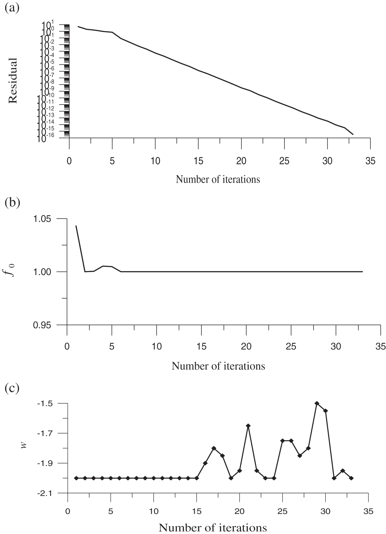
Figure 3: For test case 3, (a) display the residual plot, (b) the minimum value of the merit function, and (c) the optimized value of the splitting parameter
Here, considering the following boundary value problem:
The exact solution is
By using the finite difference discretisation of u at the grid points, we can obtain
where
Setting n = 39,
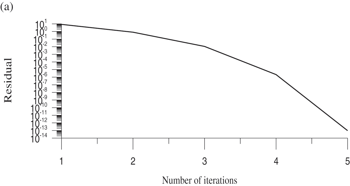
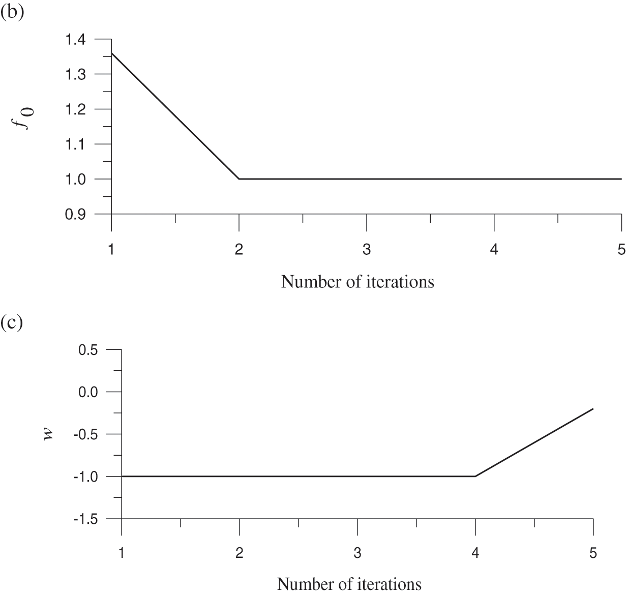
Figure 4: For test case 4, (a) display the residual plot, (b) the minimum value of the merit function, and (c) the optimized value of the splitting parameter
Then, considering a test example given by Krzyworzcka [30] as follows:
To convince describe the coefficient matrices of B as Eq. (21),
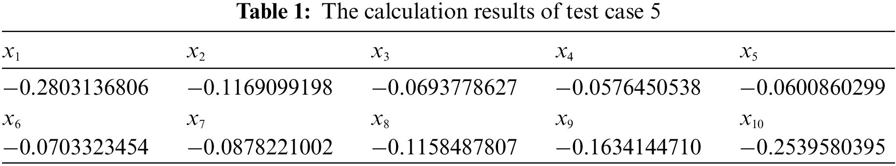
Setting
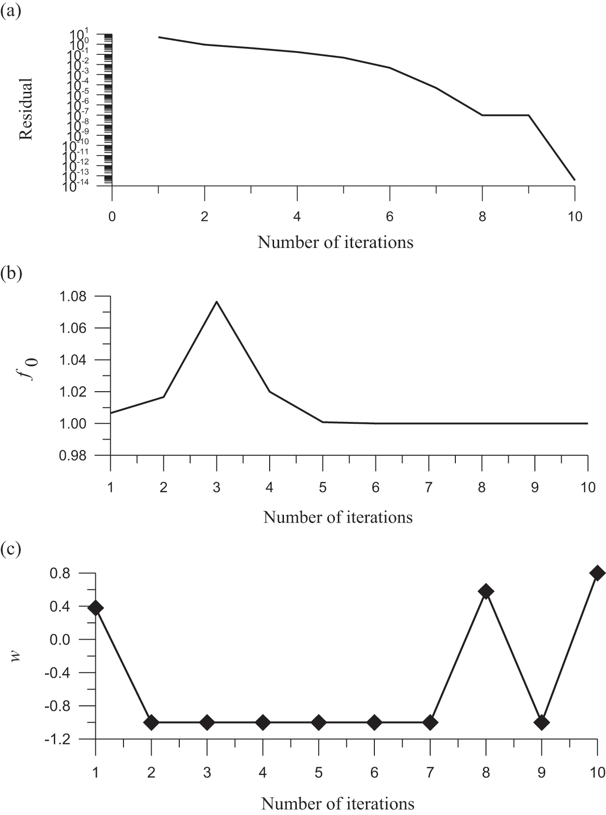
Figure 5: For test case 5, (a) display the residual plot, (b) the minimum value of the merit function, and (c) the optimized value of the splitting parameter
The following example is given by Roose et al. [31]:
The OSLIM can adopt two different formulations to solve Eq. (53). The two different formulations lead to different coefficient matrices of B. First, we adopt
To convince desdescribee coefficient matrices of B as Eq. (21),
where the number with a superscript k denotes the kth step value, and it is inserted in the coefficient matrix when we derive the linear system. We modify the term
in the second line to
such that we have a second formulation:
To convince describe the coefficient matrices of B as Eq. (21),
Setting n = 10,
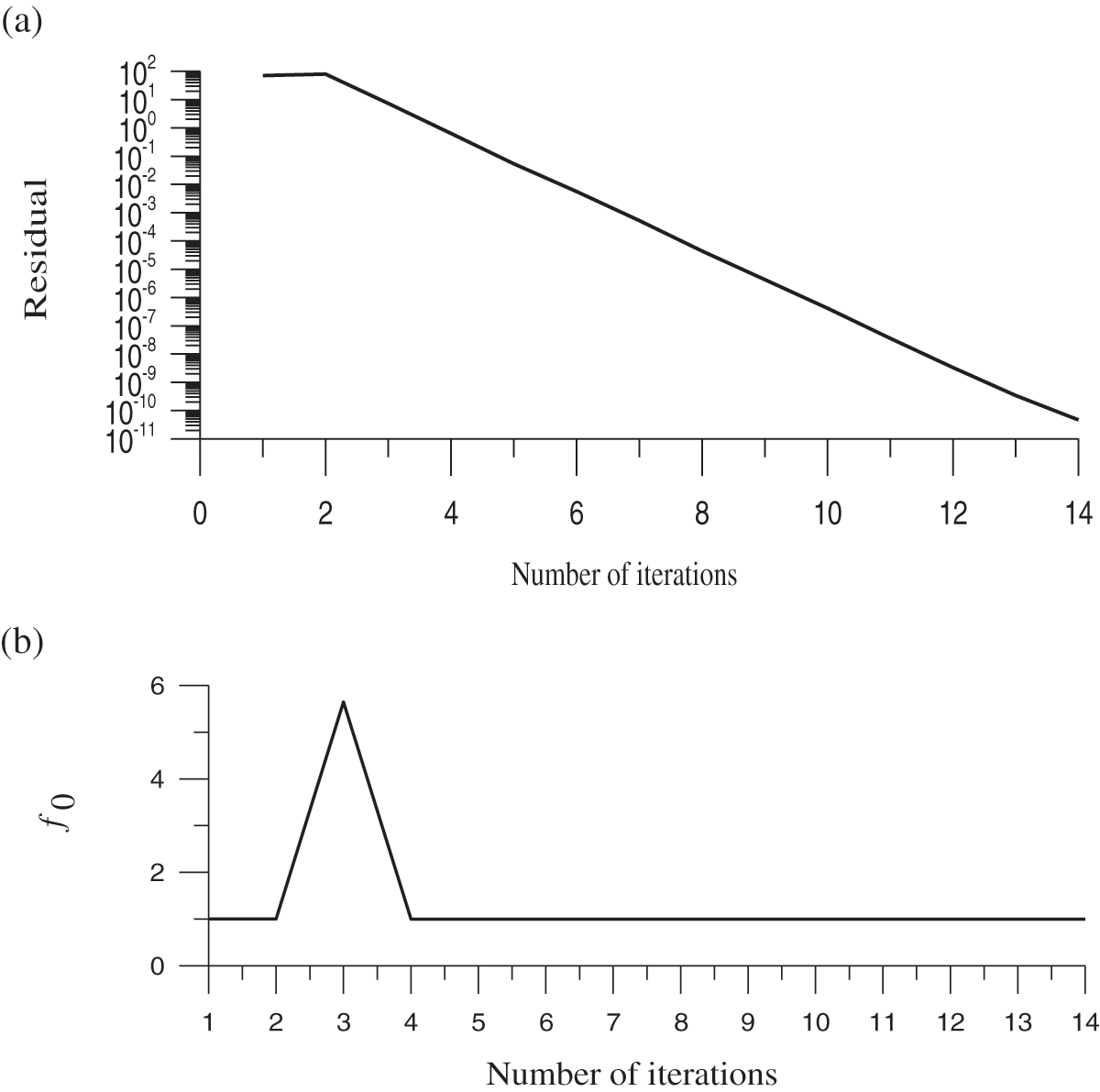
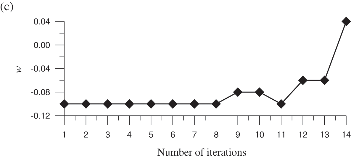
Figure 6: For test case 6, (a) display the residual plot, (b) the minimum value of the merit function, and (c) the optimized value of the splitting parameter
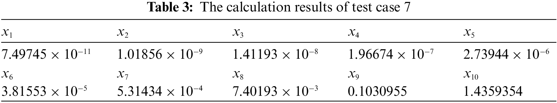
Setting n = 10,
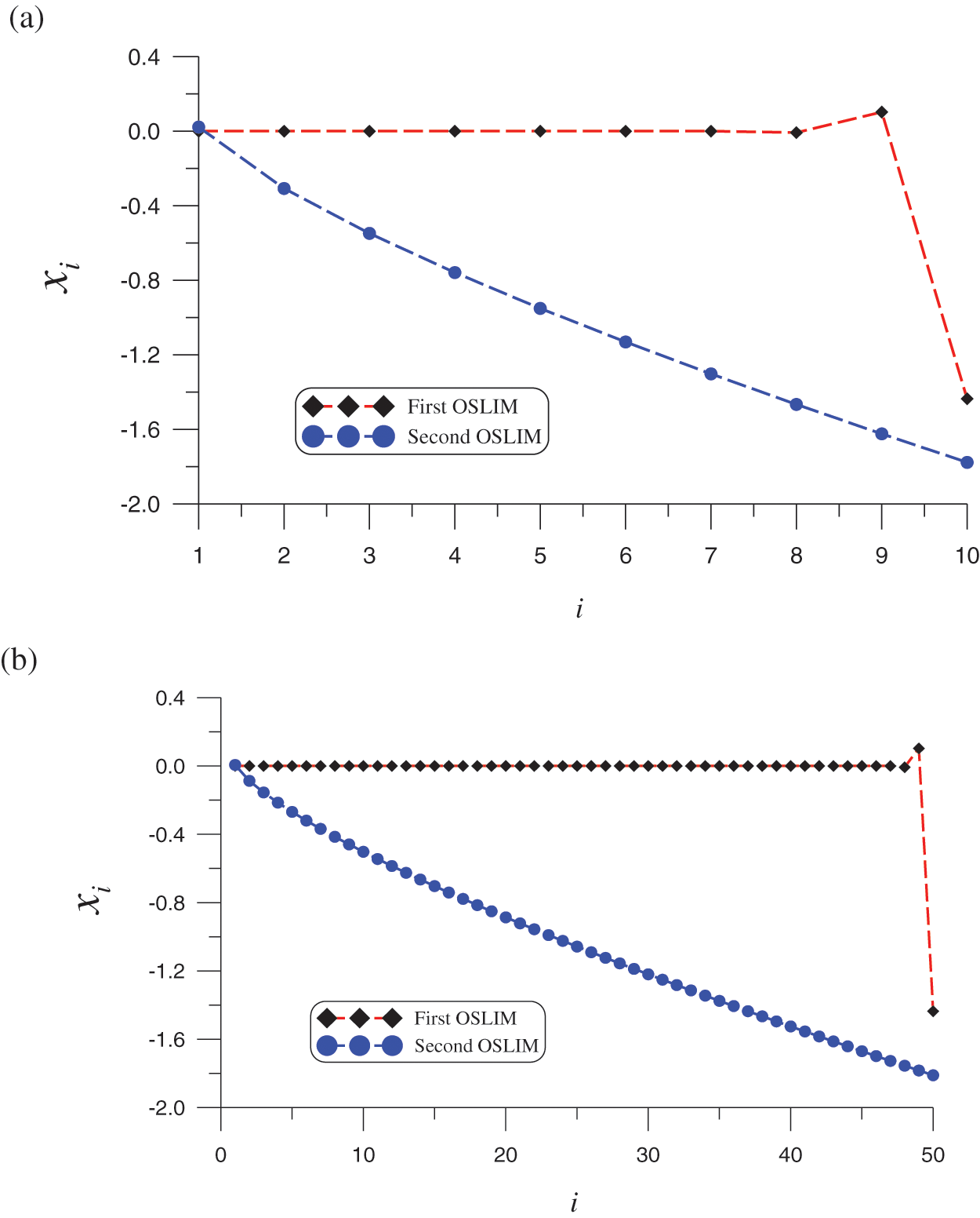
Figure 7: For test case 6, comparing two different solutions obtained by the first OSLIM and the second OSLIM: (a) n = 10, and (b) n = 50
Considering the following a two-dimensional nonlinear Bratu equation:
and the domain is an ellipse with semi-axes lengths a = 1 and b = 0.5. The Dirichlet boundary condition is imposed. Due to u > 0, we decompose it to
where
After collocating points inside the domain and on the boundary, simultaneously, to satisfy the Eq. (56) and the boundary condition equation, we can derive NAEs to determine the
By using the OSLIM, we take
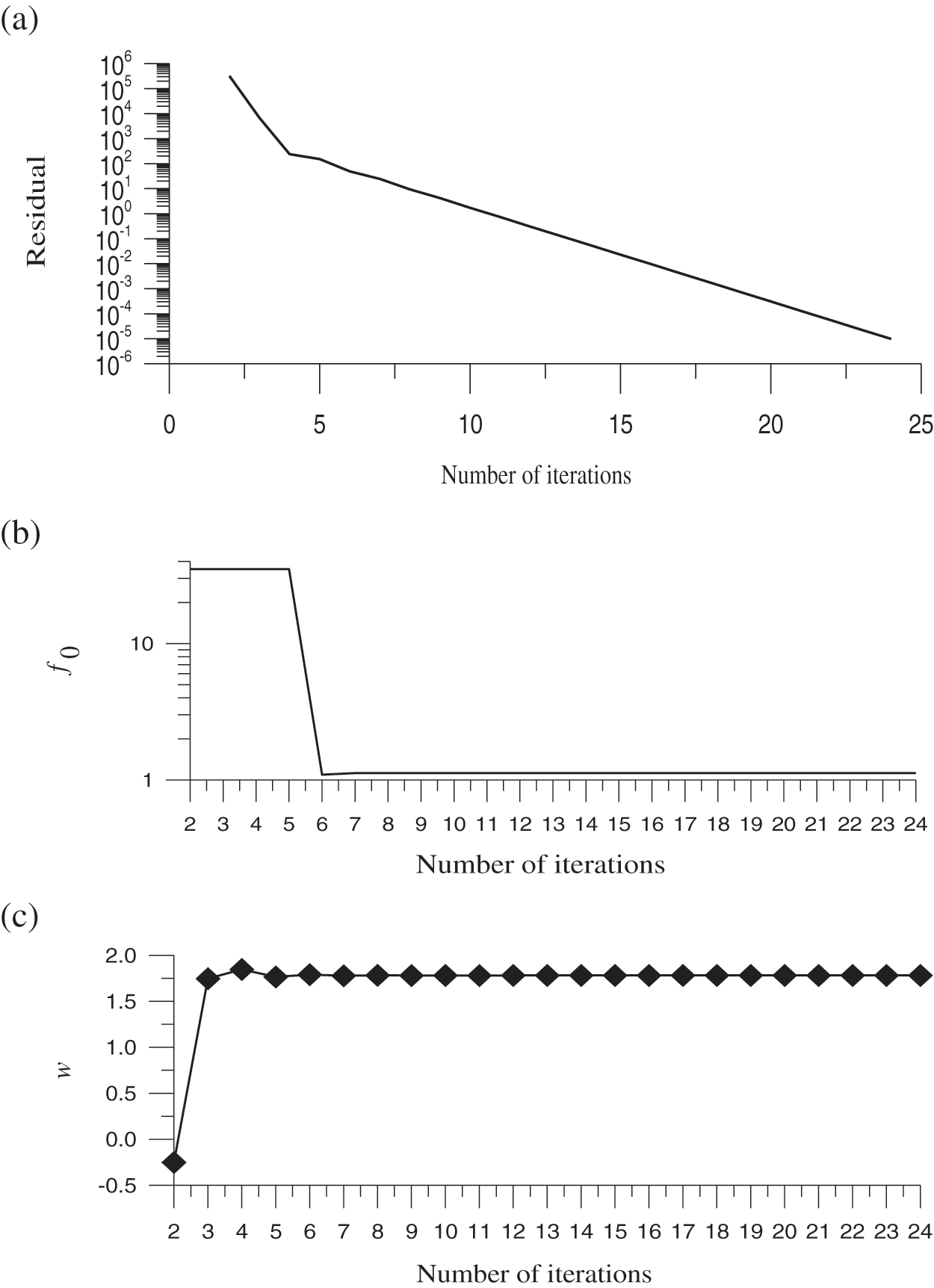
Figure 8: For test case 7, (a) display the convergence plot, (b) the minimum value of the merit function, and (c) the optimized value of the splitting parameter
When evaluating the performance of newly developed iterative solutions for solving nonlinear algebraic equations (NAE), there are two critical factors: accuracy and convergence speed. In this article, we first decomposed the nonlinear terms in the NAEs through a splitting parameter and then we linearized the NAEs around the values at the previous step and derived a system of linear algebraic equations (LAEs). Through the maximum orthogonal projection concept at each iterative step, we select the optimal value of the splitting parameter and use the Gaussian elimination method to solve the LAE. The features of the proposed method are summarized as follows: (a) The merit function is in terms of the coefficient matrix, right-side vector and the value of unknown vector at the previous step. (b) It is easy to minimize the search within a preferred interval through some operations. (c) The current OSLIM is insensitive to the initial guess and without needing the inversion of the Jacobian matrix at each iterative step, which can save much of the computational time. We have successfully applied the OSLIM to solve the NAEs resulting from the nonlinear boundary value problem in one- and two-dimensional spatial spaces. Through the numerical test, the convergence order of the OSLIM is between linear and quadratic convergence.
Funding Statement: The corresponding author appreciates the financial support provided by the Ministry of Science and Technology, Taiwan, ROC under Contract No. MOST 110-2221-E-019-044.
Conflicts of Interest: The authors declare that they have no conflicts of interest to report regarding the present study.
References
1. Liu, C. S., Atluri, S. N. (2008). A fictitious time integration method (FTIM) for solving mixed complementarity problems with applications to non-linear optimization. Computer Modeling in Engineering & Sciences, 34(2), 155–178. DOI 10.3970/cmes.2008.034.155. [Google Scholar] [CrossRef]
2. Kwak, B. M., Kwak, J. Y. (2021). Binary NCP: A new approach for solving nonlinear complementarity problems. Journal of Mechanical Science and Technology, 35(3), 1161–1166. DOI 10.1007/s12206-021-0229-5. [Google Scholar] [CrossRef]
3. Shih, C. F., Chen, Y. W., Chang, J. R., Soon, S. P. (2021). The equal-norm multiple-scale trefftz method for solving the nonlinear sloshing problem with baffles. Computer Modeling in Engineering & Sciences, 127(3), 993–1012. DOI 10.32604/cmes.2021.012702. [Google Scholar] [CrossRef]
4. Nurhidayat, I., Hao, Z., Hu, C. C., Chen, J. S. (2020). An ordinary differential equation approach for nonlinear programming and nonlinear complementarity problem. International Journal of Industrial Optimization, 1(1), 1–14. DOI 10.12928/ijio.v1i1.764. [Google Scholar] [CrossRef]
5. Fischer, A. (1992). A special newton-type optimization method. Optimization, 24(3–4), 269–284. DOI 10.1080/02331939208843795. [Google Scholar] [CrossRef]
6. Liu, C. S., Atluri, S. N. (2008). A novel time integration method for solving a large system of non-linear algebraic equation. Computer Modeling in Engineering & Sciences, 31(2), 71–83.15. DOI 10.3970/CMES.2008.031.071. [Google Scholar] [CrossRef]
7. Liu, C. S. (2009). A fictitious time integration method for a quasilinear elliptic boundary value problem, defined in an arbitrary plane domain. Computers, Materials & Continua, 11(1), 15–32. DOI 10.3970/cmc.2009.011.015. [Google Scholar] [CrossRef]
8. Liu, C. S. (2001). Cone of non-linear dynamical system and group preserving schemes. International Journal of Non-Linear Mechanics, 36, 1047–1068. DOI 10.1016/S0020-7462(00)00069-X. [Google Scholar] [CrossRef]
9. Atluri, S. N., Liu, C. S., Kuo, C. L. (2009). A modified newton method for solving non-linear algebraic equations. Journal of Marine Science and Technology, 17(3), 238–247. DOI 10.51400/2709-6998.1960. [Google Scholar] [CrossRef]
10. Jones, C., Tian, H. (2017). A time integration method of approximate fundamental solutions for nonlinear poisson-type boundary value problems. Communications in Mathematical Sciences, 15(3), 693–710. DOI 10.4310/CMS.2017.v15.n3.a6. [Google Scholar] [CrossRef]
11. Hashemi, M. S., Mustafa, I., Parto-Haghighi, M., Mustafa, B. (2019). On numerical solution of the time-fractional diffusion-wave equation with the fictitious time integration method. European Physical Journal Plus, 134, 488. DOI 10.1140/epjp/i2019-12845-1. [Google Scholar] [CrossRef]
12. Demmel, J. W. (1997). Applied numerical linear algebra. Philadelphia: SIAM. [Google Scholar]
13. Saad, Y. (2003). Iterative methods for sparse linear systems. Philadelphia: SIAM. [Google Scholar]
14. Quarteroni, A., Sacco, R., Saleri, F. (2000). Numerical mathematics. New York: Springer Science. [Google Scholar]
15. Hadjidimos, A. (2000). Successive overrelaxation (SOR) and related methods. Journal of Computational and Applied Mathematics, 123(1–2), 177–199. DOI 10.1016/S0377-0427(00)00403-9. [Google Scholar] [CrossRef]
16. Bai, Z. Z., Chi, X. B. (2003). Asymptotically optimal successive overrelaxation method for systems of linear equations. Journal of Computational Mathematics, 21(5), 603–612. [Google Scholar]
17. Wen, R. P., Meng, G. Y., Wang, C. L. (2013). Quasi-Chebyshev accelerated iteration methods based on optimization for linear systems. Computers & Mathematics with Applications, 66(6), 934–942. DOI 10.1016/j.camwa.2013.06.016. [Google Scholar] [CrossRef]
18. Meng, G. Y. (2014). A practical asymptotical optimal SOR method. Applied Mathematics and Computation, 242, 707–715. DOI 10.1016/j.amc.2014.06.034. [Google Scholar] [CrossRef]
19. Miyatake, Y., Sogabe, T., Zhang, S. L. (2020). Adaptive SOR methods based on the wolfe conditions. Numerical Algorithms, 84, 117–132. DOI 10.1007/s11075-019-00748-0. [Google Scholar] [CrossRef]
20. Yang S., G., K, M. (2009). The optimal relaxation parameter for the SOR method applied to the poisson equation in any space dimensions. Applied Mathematics Letters, 22(3), 325–331. DOI 10.1016/j.aml.2008.03.028. [Google Scholar] [CrossRef]
21. Liu, C. S. (2020). A new splitting technique for solving nonlinear equations by an iterative scheme. Journal of Mathematics Research, 12(4), 40–48. DOI 10.5539/jmr.v12n4p40. [Google Scholar] [CrossRef]
22. Liu, C. S., Hong, H. K., Lee, T. L. (2021). A splitting method to solve a single nonlinear equation with derivative-free iterative schemes. Mathematics and Computers in Simulation, 190, 837–847. DOI 10.1016/j.matcom.2021.06.019. [Google Scholar] [CrossRef]
23. Liu, C. S. (2012). A globally optimal iterative algorithm to solve an ill-posed linear system. Computer Modeling in Engineering & Sciences, 84(4), 383–403. DOI 10.3970/cmes.2012.084.383. [Google Scholar] [CrossRef]
24. Liu, C. S. (2013). An optimal tri-vector iterative algorithm for solving ill-posed linear inverse problems. Inverse Problems in Science and Engineering, 21, 650–681. DOI 10.1080/17415977.2012.717077. [Google Scholar] [CrossRef]
25. Liu, C. S. (2014). A globally optimal tri-vector method to solve an ill-posed linear system. Journal of Computational and Applied Mathematics, 260, 18–35. DOI 10.1016/j.cam.2013.09.017. [Google Scholar] [CrossRef]
26. Yeih, W. C., Ku, C. Y., Liu, C. S., Chan, I. Y. (2013). A scalar homotopy method with optimal hybrid search directions for solving nonlinear algebraic equations. Computer Modeling in Engineering & Sciences, 90(4), 255–282. DOI 10.3970/cmes.2013.090.255. [Google Scholar] [CrossRef]
27. Chen, Y. W. (2014). A residual-norm based algorithm for solving determinate/indeterminate systems of non-linear algebraic equations. Journal of Marine Science and Technology, 22(5), 583–597. DOI 10.6119/JMST-013-0912-1. [Google Scholar] [CrossRef]
28. Hirsch, M., Smale, S. (1979). On algorithms for solving f(x) = 0. Communications on Pure & Applied Mathematics, 32(3), 281–312. DOI 10.1002/cpa.3160320302. [Google Scholar] [CrossRef]
29. Liu, C. S., Atluri, S. N. (2011). An iterative algorithm for solving a system of nonlinear algebraic equations,
30. Krzyworzcka, S. (1996). Extension of the lanczos and CGS methods to systems of nonlinear equations. Journal of Computational and Applied Mathematics, 69(1), 181–190. DOI 10.1016/0377-0427(95)00032-1. [Google Scholar] [CrossRef]
31. Roose, A., Kulla, V., Lomb, M., Meressoo, T. (1990). Test examples of systems of non-linear equations. Tallin: Estonian Software and Computer Service Company. [Google Scholar]
Cite This Article
 Copyright © 2023 The Author(s). Published by Tech Science Press.
This work is licensed under a Creative Commons Attribution 4.0 International License , which permits unrestricted use, distribution, and reproduction in any medium, provided the original work is properly cited.
 Downloads
 Citation Tools