Machine Learning-Based Channel State Estimators for 5G Wireless Communication Systems

1  Introduction

In the subsequent years, it is expected that exponential growth in wireless throughput for different wireless services will continue. 5G communication systems have been designed to meet the vast increase in data traffic and achieve robust communications under the conditions of non-stationary channel statistics. 5G-orthogonal frequency division multiplexing (OFDM) communication systems have been deployed to mitigate the frequency selective fading effects and other channels imperfections, resulting in offering more reliable communication systems and increasing the spectrum efficiency significantly [1].

One of the most important factors affecting the effectiveness of CSEs is a priori information about the wireless communication channel environment provided by pilots. Both the transmitter and receiver should know the pilot signals to estimate the communication channel information and efficiently recover the desired signal. Channel state estimate is worthless if no or inadequate a priori knowledge is available (no or limited pilots) [2].

Least squares (LS) estimation is well-known among conventional channel state estimators has a low computational cost since it requires no prior channel information. On the other hand, the LS estimator produces substantial errors of channel estimation in real applications, particularly for multipath channels. Minimum mean square error (MMSE) CSE, grants the best channel information estimation compared with LS CSE [3,4]. MMSE-based estimations assume the linearity of the experienced transmission channel, and the Gaussian probability density function describes all channel responses [2]. The mean and covariance values of communication channels are challenging to get or change fast in a short coherence time in many propagation environments, making the MMSE estimation challenging to implement [3].

Deep learning neural networks-based wireless communication applications recently received a lot of attention, such as coding and decoding, automatic signals classification, MIMO detection, and channel estimation [2,5–11]. As a result, several deep learning algorithms, such as recurrent neural networks (RNNs) (e.g., LSTM and BiLSTM NNs), convolutional neural networks (CNNs), and hybrid CNN and RNN structures, have utilized to estimate the channel state in 5G wireless communication networks.

In [12], the channel response feature vectors and channel estimation were extracted using CNN and BiLSTM deep learning-based estimators, respectively. The main target was to enhance the estimate performance at the downlink, in communication environments concerning high-speed mobility. In [13], an online-trained CSE that integrates CNN and LSTM have developed. In addition, the authors have developed a way for combining offline and online learning for 5G systems. In [5], for OFDM systems which deal with frequency selective channels, a feedforward DLNN-based joint CSE was presented. When uncertain imperfections are taken into account, the suggested approach outperforms the classic MMSE estimate technique. In [14], Feedforward DNNs were used to develop an online CSE for doubly selective channels. The suggested CSE was found to be better than the classic LMMSE one in all circumstances studied. In [8], 1D-CNN-based CSE have introduced. Using different modulation methods, the authors compared the proposed estimator performance against FFNN, MMSE, and LS CSEs in terms of MSE and BER. 1D-CNN outstripped the conventional, and FFNN CSEs. In [9], A recurrent LSTM deep learning neural network was employed to construct an online CSE for OFDM communication systems. The developed estimator is dependent on pilots’ utilization. The suggested CSE achieved superior performance than the conventional estimators using a small number of pilots and uncertain channel models. Sarwar et al. [15] built a CSE using a genetic algorithm-optimized artificial neural network. The suggested estimator was designed for MIMO-OFDM systems that use space-time block-coding. The provided CSE outperformed both LS and MMSE estimators at high signal-to-noise ratios (SNRs), but it performed similarly at low ones. Senol et al. [16] have proposed ANN-based CSE for sparsely multipath channels. The suggested estimator outperformed both matching and orthogonal matching pursuit-based CSEs in terms of SER while having a reduced computational complexity. Le et al. [17] have proposed two fully-connected DNN (FDNN)-based CSE structures for a 5G MIMO-OFDM system over frequency-selective fading channels. Two alternative scenarios depending on the receiver velocity are then used to test the performance of the proposed CSEs. The tapped delay line type A model (TDL-A), which is provided by 3GPP and covers realistic situations, is used to produce channel parameters in each scenario. The two proposed FDNN-based CSEs are compared to the standard LS and Linear MMSE estimations. Le et al. [18] expanded their previous work in [17] by proposing DNN-based CSEs that use a neural network to learn the characteristics of real channels using the channel estimates produced using LS estimation as input. They use three different DNN structures: FDNN, CNN, and bi-LSTM. The performance of the three DNN-based CSEs was numerically evaluated, and their usefulness was shown by comparing them to classic LS and LMMSE CSEs. Li et al. [19] proposed a denoising autoencoder DNN-based CSE to mitigate the presence of impulsive noise in OFDM systems, since impulsive noise may cause a serious decline in channel estimation performance. The simulation findings showed that the proposed CSE improves the OFDM channel information estimation process and outperforms the existing peers, such as LS, MMSE, and orthogonal matching pursuit CSEs. Hu et al. [20] did some preliminary research on deep learning-based channel estimation for single-input multiple-output (SIMO) systems to better understand and explain their internal mechanisms. Using the ReLU activation function efficiently, the suggested estimator can approximate a vast family of functions. They show that the suggested CSE is not restricted to any particular signal model and may be used to estimate MMSE in numerous contexts. The findings show that the DL CSE based on ReLU DNNs may closely mimic the MMSE CSE with numerous training samples. Coutinho et al. [21] suggested employing CNNs without forward error correction codes to solve the issue of cascaded channel state estimation in 5G and future communication systems. The findings reveal that the proposed CNN-based CSE approaches perfect (theoretical) channel estimation levels in terms of bit error rate (BER) values and beats LS practical estimation in terms of mean squared error (MSE). Xiong et al. [22] presented a novel real-time CNN-based CSE that uses the latest reference signal (RS) for online training and extracts the temporal features of the channel, followed by prediction employing the optimal model. For high-speed moving scenarios, the proposed CSE is used in OFDM systems, such as long-term evolution (LTE) and 5G systems, to track the fast time-varying and non-stationary channels using a real-time RS-based training algorithm and obtain an accurate CSI without changing the radio frame. Experiments show that the proposed CSE outperforms conventional peers, and that even more improvement is possible at higher speeds.

In this work, we expand our preceding research work [2] and [9]. In [9] the focus was on proposing the online LSTM-based CSE for OFDM wireless communication systems. A comparative study was conducted utilizing the adaptive moment estimation (Adam), root mean square propagation (RMSProp), and stochastic gradient descent with momentum (SGdm) optimization algorithms to assess the performance of the proposed estimator. Compared to the conventional estimators, the suggested estimator outperforms at a few pilots. In [2] a pilot-dependent estimator for 5G OFDM and coming systems have proposed by employing deep learning BiLSTM neural networks. This work was the first to develop the recurrent BiLSTM NN-based CSE without integration with CNN. As a result, the developed CSE requires no prior knowledge of channel characteristics and performs well using small pilots. In addition, two novel classification layers were proposed using loss functions: mean absolute error and sum of squared of the errors. Finally, the proposed BiLSTM estimator was compared to the most utilized LS and MMSE; and LSTM CSEs. The findings revealed that the BiLSTM CSE performs similarly to the MMSE CSE using many pilots and outperforms the conventional peers at a few pilots. Furthermore, the suggested estimator enhances the transmission rate of OFDM systems by outperforming the other estimators using a limited number of pilots. The developed LSTM and BiLSTM CSEs are favourable for 5G and future systems.

The current study will propose a CNN DNN-based CSE for OFDM networks. This is the first time a CNN network has been used as a CSE without the use of BiLSTM or LSTM recurrent DNNs. The previous certainty of channel statistics is not required for the CNN-based CSE. The performance of the recent CNN estimator will be compared with previously developed LSTM and BiLSTM estimators, and of course, the conventional estimators in terms of symbol error rate. The comparative study between the three CNN-, BiLSTM-, and LSTM-based CSIEs will be conducted using adaptive moment estimation (Adam) optimization algorithm and three classification layers. One of the three classification layers is built using the most common loss function crossentropyex, while the other two classification layers are that proposed in [2,23]. The findings indicate that the suggested BiLSTM CSE performs similarly to the MMSE, LSTM, and CNN CSEs at many pilots. It also outperforms the LSTM, CNN, and traditional LS and MMSE CSEs at limited pilots. Furthermore, compared to the CNN, LS, and LSTM CSEs, the suggested BiLSTM and LSTM CSEs increase the transmission rate of 5G-OFDM networks because they demonstrate optimal performance at a few pilots. The proposed DNNs-based CSEs are data-driven approaches; so, they can analyze, recognize, and understand the propagation channels statistics in the presence of different imperfections.

The rest of this paper is organised as follows. The recurrent (LSTM and BiLSTM) DNN-based CSEs are illustrated in the Section 2. Section 3 explored the CNN-based CSE. The OFDM model, and offline learning concept are introduced in A and B subsections of the Section 4. The outcomes of the simulation are presented in the Section 5. The Section 6 contains the conclusions and future plans.

2  DNN-Based CSE

A recurrent BiLSTM-based CSE is provided in this part. The BiLSTM network is a variant of recurrent LSTM NN, which can learn long-term relationships between input data time steps [24–26].

The BiLSTM architecture comprises two distinct LSTM NNs with forward and backward information propagation directions. The LSTM architecture comprises input, forget, and output, gates as well as a memory cell. LSTM NN can successfully store long-term memory because to the forget and input gates. The primary structure of the LSTM cell is depicted in Fig. 1. The forget gate allows the LSTM NN to delete unwanted information from the currently utilized input xt and cell output ht of the last process. The input gate locates the data that will be utilised with the previous LSTM cell state ct−1 to obtain a new cell state ct based on the current cell input xt and the previous cell output ht−1. LSTM can pick which information to discard and which to keep using the forget and input gates.

Figure 1: Long short-term memory (LSTM) cell

The output gate determines present cell output ht by using the preceding cell output ht−1 at present cell state ct and input xt. The LSTM NN architecture model can be defined using Eqs. (1)–(6).

it=σg(wixt+Riht−1+bi),(1)

ft=σg(wfxt+Rfht−1+bf),(2)

gt=σc(wgxt+Rght−1+bg),(3)

ot=σg(woxt+Roht−1+bo),(4)

ct=ft⊙ct−1+it⊙gt,(5)

ht=ot⊙σc(ct),(6)

where i,f,g,o,σc,σg and ⊙ represent the input gate, forget gate, cell candidate, output gate, hyperbolic tangent (tanh) state activation function, sigmoid gate activation function and Hadamard product respectively. W=[wiwfwgwo]T, R=[RiRfRgRo]T and b=[bibfbgbo]Tare input weights, recurrent weights and bias, respectively.

The output unit receives both the forward and backward propagation information simultaneously. As a result, as illustrated in Fig. 2, previous and future information may be recorded. At time t, the input is delivered to forward and backward LSTM networks. BiLSTM NN final output may be stated as follows:

Figure 2: BiLSTM-NN architecture

ht=h→t⊙h←t,(7)

where h→t is forward output and h←t is backward output of BiLSTM architecture.

The constructed BiLSTM-based CSE uses a cross-entropy function for the kth mutually exclusive class (crossentropyex)-based classification layer as the last CSE layer. In addition, authors have been developed a mean absolute error (MAE)-based classification layer and a sum of squared errors (SSE)-based classification layer [2]. Finally, the suggested estimator’s weights and biases are optimized using the adaptive moment estimation (Adam) optimization algorithm and each of the classification layers, seeking to get the most accurate and robust CSE under the conditions of uncertain channel statistics and restricted pilots.

An array with the following five layers is used to construct the BiLSTM NN-based channel state estimator: sequence input, BiLSTM, fully connected, softmax, and output classification. The maximum input size was set at 256. The BiLSTM layer comprises 16 hidden units and displays the last element of the sequence. The size four fully connected (FC) layer, followed by a softmax layer, and finally a classification layer, specifies four classes. The construction of the suggested BiLSTM and LSTM estimators is seen in Fig. 3.

Figure 3: Structure of BiLSTM and LSTM estimators

3  CNN-Based CSE

CNN architectures have been suggested for image denoising techniques and have received significant attention in the image processing field. CNN architectures may learn how to map noisy images to clean images [27], hence reducing image noise. A CNN can also reduce the number of parameters by sharing its biases and weights, and thus reducing the system’s complexity. CNN can be trained to map noisy channels to genuine channels based on these notions. The CNN-based channel state estimator weights and biases will be updated during the training phase by minimizing one of the three loss functions (13)–(15). Fig. 4 depicts the structure of the proposed CNN-based estimator. It has one 2D input layer, two convolution layers, two layers of batch normalization, two “ReLU” activation layers, one max pooling layer, one fully connected layer, one “Softmax” layer, and one output classification layer. These layers are depicted in Fig. 4, and briefly described in the following subsection.

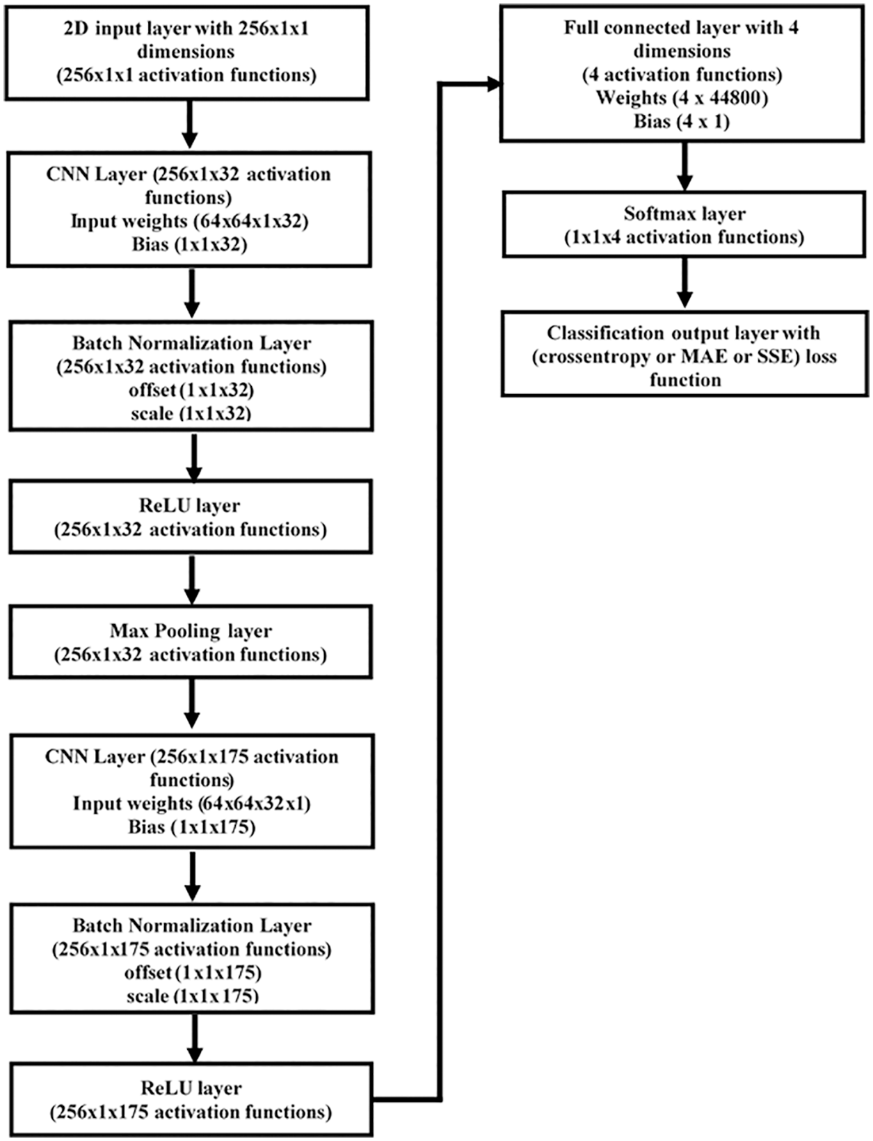
Figure 4: CNN channel state estimator structure

3.1 Convolutional Layer (CL)

In convolutional layers, there are several convolution filters to process the received signal. Assume that the lth CL of the CNN-based CSE, Ns is the number of inputs, Lsl is the input length, Nkl is the filters’ number, and Lkl is the length of filters of the lth layer. The convolution process in the lth layer is formulated as follows:

hkl=f(xl×Wkl+bkl)(8)

(xl×Wkl)(i)=∑a=−∞∞x(a)Wkl(i−a)(9)

where hl∈RNkl×Lsl represents the output set, often known as the feature map, x∈RNs×Lsl represents inputs, W∈RNkl×Lkl rpresents set of filters, b∈RNs represents the outputs’ biases, and f(.) is the activation function. It is chosen as (Relu) in the proposed estimator. The output of the kth_filter is denoted by (9), where k=1,2,…,Nkl.

3.2 Batch Normalization (BN) Layer

Deep network training may be made faster by lowering the internal covariate shift, which is achieved via the BN layer. In the context of layer training, the internal covariate shift is defined as the change in the distribution of output from each layer. Most of the time, imbalanced nonlinear mapping is to blame for the changes. Frequently the BN layer is exploited before the activation function when it is suggested.

3.3 ReLU Layer

The activation function serves as a way to map outputs in a nonlinear fashion. Sigmoid and tanh are the most common use activation function. In this paper the rectified linear unit (ReLU) is adopted as the activation function, it can be defined as

f(x)={x,x≥00,x<0(10)

3.4 Max-Pooling Layer

In CNN, the pooling layer is an essential sort of layer. The convolutional layer uses many convolutions to generate a series of outputs, each of which is run using the (ReLU) function. The layer’s output is then further modified using a pooling mechanism. A pooling function substitutes a net’s output at a particular position with a summary statistic of neighboring outputs. In this research, max pooling is employed, which reports the highest output inside a pooling window.

3.5 Full Connected Layer

A fully connected (FC) layer multiplies the input by a weight matrix and then adds a bias vector. In this paper, the convolutional layer is followed by one FC layer. In a FC layer, all neurons are connected to all the neurons in the previous layer. This layer combines all the features learned by the previous layers across the transmission channel to estimate the channel information. For channel state estimation problems, the last FC layer combines the features to estimate the information state of a particular channel.

3.6 Output (Softmax and Classification) Layers

A softmax layer applies a softmax function to the input. The softmax function is the output unit activation function after the last FC layer for multi-class classification problems. It is also known as the normalized exponential and can be considered the multi-class generalization of the logistic sigmoid function.

For typical classifiers, the classification layer generally comes after the softmax layer. During the training process, in the classification layer, the optimization algorithm receives the outputs from the softmax function and assigns each input to one of the K mutually exclusive classes using the crossentropy function for a 1-of-K coding scheme.

4  DNNs-Based CSEs for 5G–OFDM Systems

The next subsections describe the conventional OFDM wireless communication technology as well as deep offline learning of the proposed channel state estimators.

4.1 OFDM Model

Fig. 5 depicts the construction of the classic OFDM system [9].

Figure 5: Conventional OFDM system [9]

A serial-to-parallel (S/P) converter is utilized on the transmitter side to transform the transmitted symbols with pilot signals into parallel data streams. Then, inverse discrete Fourier transform (IDFT) transforms the signal into the time domain. Finally, to mitigate the effects of inter-symbol interference (ISI), a cyclic prefix (CP) must be inserted. The CP length must be greater than the channel’s maximum spreading delay.

A multipath channel formed by complicated random variables in a sample space {h(n)}n=0N−1 is counted. Subsequently, the received signal can be calculated using the following formula:

y(n)=x(n)⊕h(n)+w(n),(11)

where x(n) ⊕, w(n), y(n) are input signal, circular convolution, additive white Gaussian noise and output signal, respectively.

In the frequency domain, the received signal may be described as

Y(k)=X(k)H(k)+W(k),(12)

where the DFT of x(n), h(n), y(n) and w(n) are X(k), H(k), Y(k) and W(k), correspondingly. These DFTs are calculated after CP eliminating.

The pilot symbols from the first OFDM block are included in the OFDM frame and the transmitted data from the subsequent blocks. The channel may appear stationary during one frame, yet it can shift between frames. The offered BiLSTM-based CSE accepts data at its input and recovers it at its output [5,9].

4.2 Offline Learning of the DNNs-Based CSEs

In the realm of wireless communication, DNNs are the state-of-the-art technique, but they have high computational complexity and a lengthy training period. The most dominant devices for training DNNs are GPUs [28]. Because of the proposed CSE’s long training time and the vast number of BiLSTM NN biases and weights that must be optimized the training process should be done offline. The trained channel state estimator is then used to extract the transmitted data in an online implementation [5,9].

The learning dataset for one subcarrier is randomly generated during offline training. Through the adopted channel, the transmitting end sends OFDM frames to the receiving end. The received signal is retrieved using transmitted frames that have been exposed to various channel defects.

Traditional CSEs are strongly reliant on theoretical channel models that are linear, stable, and follow Gaussian statistics. However, existing wireless systems contain other flaws and unidentified circumferent effects that are difficult to account for with precise channel models; as a result, researchers have created several channel models that accurately characterize practical channel statistics. Modelling may produce trustworthy and practical training datasets utilizing these channel models [9,29,30].

In The 3GPP-5G TR 38.901 version 16.1.0 Release 16 channel model [30] is utilized to mimic the behaviour of the practical transmission channel in wireless systems. Specifically, we use the tapped delay line (TDL) models with the carrier frequency, fc = 2.6 GHz, the sampling rate, the number of main paths, L = 24, and the number of subcarriers, K = 64. The considered channel model simulates both the frequency-selective fading and time-selective fading caused by multipath and Doppler shifting, respectively.

Adam optimization trains the proposed CSEs by minimizing a specific loss function. The difference between the estimator’s reactions and the originally sent data is defined as a loss function. A variety of functions can represent the loss function. The loss function is an indispensable part of the classification layer. The frequently used classification layer is mainly based on the crossentropyex loss function in MATLAB/software. Two more classification layers employ (MAE and SSE) loss functions were established in this study. The suggested estimators’ performance is studied when three classification layers are used. The used loss functions can be defined as follows:

crossentropyex=−∑i=1N∑j=1cXij(k)log⁡(X^ij(k))(13)

MAE=∑i=1N∑J=1C|Xij(k)−X^ij(k)|N(14)

SSE=∑i=1N∑J=1C(Xij(k)−X^ij(k))2(15)

where N is the number of samples, c is the number of classes, Xij(k) is the i th transmitted sample for the j th class and X^ij is the DNN-based CSE response for sample i for class j.

Fig. 6 depicts the steps involved in creating the training data sets and performing offline deep learning to create a learned CSE based on deep learning CNN, LSTM, or BiLSTM neural networks.

Figure 6: Offline learning process of the examined DNNs-based CSEs

In the offline training phase, the initially created DNN-based CSE takes the training data as pairs. Each pair consists of a specific input (transmitted data x(n) influenced by channel conditions with specific statistical characteristics (CSI)) and its corresponding received data y(n). Offline training results in learned DNN-based CSE, which in sequence is used in the deployment phase where the trained model accepts the observed signal y(n) and successfully retrieves the original transmitted data x(k) without explicitly estimating the wireless channel.

5  Results of Simulation

5.1 Analyzing the Effectivness of the Conventional and DNNs-Based CSEs

Many simulations are carried out to assess the performance of the suggested estimators. The proposed DNN-based (CNN, LSTM [9], and BiLSTM [2]) estimators’ SER performance is compared to that of the optimal conventional LS and MMSE estimators. Conventional CSEs exploit the statistical information of the transmission channel to recover original data streams at receiving end. However, for all current simulations. As far to the authors’ knowledge, it is the first study to present and examine the CNN-based CSE’s performance without integration with other deep NN approaches using a few pilots. Furthermore, the Adam optimization algorithm trains the suggested estimators by employing various classification layers to get the most reliable channel state estimator among the examined ones. Finally, 2019b MATLAB/software is used to implement the suggested estimators.

The properties of the provided DNNs-based CSEs, as well as their training settings, are listed in Table 1. A trial-and-error method is used to determine these parameters. The OFDM system and channel model properties are listed in Table 2.

The CNN architecture consists of two 2D-convolution layers (2D-CL) and a single FC layer. First, 2D-CL is followed by a batch normalization (BN) layer, the rectified linear unit (ReLU) activation layer, and max-pooling layer. The second 2D-CL is followed by a BN layer, ReLU layer, and F. C. layer with size 4. The softmax activation is in the output layer. CNN’s training options such as loss functions-based classification layers, mini-batch size, epoch number, learning algorithm are the same as in Table 1.

The performance of the analyzed estimators is assessed using crossentropyex, MAE, and SSE-based classification layers and 4, 8, and 64 pilots. For all simulation investigations, the Adam optimization algorithm is employed.

Using the crossentropyex-based classification layer and enough pilots (64), the developed BiLSTM(crossentropyex) CSE beats LSTM(crossentropyex), CNN(crossentropyex), and conventional CSEs throughout the whole SNRs, as depicted in Fig. 7.

Figure 7: Comparison of the DNNs-based and conventional CSEs at pilots of 64 and the crossentropyex-based classification layer

Fig. 8 shows that using the MAE-based classification layer and a pilot number of 64, CNNMAE outperforms both BiLSTM(MAE), and LSTM(MAE). The BiLSTM(MAE), and LSTM(MAE) CSEs outperform the LS CSE throughout the SNRs of [0–18 dB], and [0–15 dB], respectively. The BiLSTM(MAE), LSTM(MAE), and CNN(MAE) estimators are comparable to the MMSE CSE throughout the SNRs of [0–10 dB], [0–4 dB], and [0–12 dB], respectively. The MMSE CSE outperforms the others outside these SNRs.

Figure 8: Comparison of the DNNs-based and conventional CSEs at pilots of 64 and the MAE-based classification layer

When the same number of pilots are used and the SSE-based classification layer is employed, Fig. 9 illustrates that the BiLSTM(SSE), LSTM(SSE), CNN(SSE), and MMSE CSEs are on par at low SNRs [0–7 dB]. Also, the MMSE CSE outstrips both BiLSTM(SSE) and LSTM(SSE) CSEs from 8 dB. The LS CSE beats LSTM(SSE), BiLSTM(SSE), and CNN(SSE) starting from 13, 15, and 18 dB, respectively. BiLSTM(SSE) outperforms LSTM(SSE) starting from 9 dB, while CNN(SSE) outperforms both BiLSTM(SSE) and LSTM(SSE) starting from 8 dB.

Figure 9: Comparison of the DNNs-based and conventional CSEs at pilots of 64 and the SSE-based classification layer

Concisely, at pilots (64), BiLSTM(crossentropyex) outperforms all examined MMSE, LSTM(crossentropyex), LSTM(MAE), LSTM(SSE), CNN(crossentropyex), CNN(MAE), CNN(SSE), and LS estimators. Furthermore, at low SNRs to 7 dB, BiLSTM(crossentropyex), BiLSTM(MAE), BiLSTM(SSE), LSTM(crossentropyex), LSTM(MAE), LSTM(SSE), CNN(crossentropyex), CNN(MAE), CNN(SSE) and MMSE CSEs achieve similar performances.

As LS does not exploit channel statistics priorly in the estimation phase, it performs poorly compared to MMSE. Conversely, MMSE exhibits superior performance using second-order channel statistics, especially with sufficient pilot numbers.

At 8 pilots, Figs. 10–12 illustrate that the developed BiLSTM(crossentropyex), BiLSTM(MAE), BiLSTM(SSE) CSEs beat LSTM(crossentropyex), LSTM(MAE), LSTM(SSE), CNN(crossentropyex), CNN(MAE), CNN(SSE) and the conventional CSEs at examination SNRs. At low SNRs to 7 dB, the presented BiLSTM(crossentropyex), BiLSTM(MAE), BiLSTM(SSE) CSEs deliver comparable performance. Furthermore, the developed BiLSTM(SSE) beats the BiLSTM(crossentropyex), and BiLSTM(MAE) CSEs. Also, it is clear that CNN(crossentropyex), CNN(MAE), and CNN(SSE) estimators suffer due to limited pilots and providing such a lousy performance compared to all examined estimators.

Figure 10: Comparison of the DNNs-based and conventional CSEs at pilots of 8 and the crossentropyex-based classification layer

Figure 11: Comparison of the DNNs-based and conventional CSEs at pilots of 8 and the MAE-based classification layer

Figure 12: Comparison of the DNNs-based and conventional CSEs at pilots of 8 and the SSE-based classification layer

At 4 pilots, Figs. 13–15 demonstrate the effectiveness of the provided BiLSTM(crossentropyex), BiLSTM(MAE), and BiLSTM(SSE) estimators compared to the examined estimators. They also show the superiority of BiLSTMSSE over BiLSTM(crossentropyex), BiLSTM(MAE), LSTM(crossentropyex), LSTM(MAE), and LSTM(SSE). At SNRs to 3 dB, the presented BiLSTM(crossentropyex), BiLSTM(MAE), and BiLSTM(SSE) CSEs deliver comparable performance. Also, it is clear that CNN(crossentropyex), CNN(MAE), and CNN(SSE) estimators have slightly better performance than the conventional estimators starting from 8 dB, but they are still suffering from the limited pilots.

Figure 13: Comparison of the DNNs-based and conventional CSEs at pilots of 4 and the crossentropyex-based classification layer

Figure 14: Comparison of the DNNs-based and conventional CSEs at pilots of 4 and the crossentropyex-based classification layer

Figure 15: Comparison of the DNNs-based and conventional CSEs at pilots of 4 and the SSE-based classification layer

The given findings highlight the robustness of BiLSTM-based CSEs against a few pilots and priori channel statistics information uncertainty. They also show how important it is to evaluate the use of multiple loss functions-based classification layers on the training process to find the best architecture for each suggested estimator.

Fig. 16 shows that at pilots of 64, 8, and 4; the presented BiLSTMcrossentropyex, BiLSTMSSE, and BiLSTMSSE CSEs have comparable performance. Also, BiLSTMSSE performance at 8 pilots is identical to BiLSTMcrossentropyex performance at 64 pilots. Therefore, 5G OFDM systems should use the suggested estimators with limited pilots that is BiLSTMSSE to considerably improve their data transmission rate. Also, it is clear that some loss functions are preferable in some situations than others. The proposed estimator is robust to a priori uncertainty for channel statistics since it uses a training data set-driven technique.

Figure 16: Comparison of the BiLSTM-based CSEs performances at 64, 8, and 4 pilots and the presented loss functions-based classification layer

5.2 Loss Curves

Exploring the training loss curves helps effectively check the quality of the DLNNs’ training process. The loss curves deliver feedback on how the learning process is going, allowing to determine if it is worthy of continuing with the learning process or not. Figs. 17–19 illustrate the loss curves of the DNN-based CSEs (BiLSTM, LSTM, and CNN) with the three loss functions-based classification layers and pilot numbers of 64, 8, and 4. All collected results are emphasized and verified by the loss curves.

Figure 17: DNNs-based CSEs loss curves comparison at pilots of 64, Adam optimization approach and loss functions-based classification layers

Figure 18: DNNs-based CSEs loss curves comparison at pilots of 8, Adam optimization approach and loss functions-based classification layers

Figure 19: DNNs-based CSEs loss curves comparison at pilots of 4, Adam optimization approach and loss functions-based classification layers

5.3 Accuracy Calculation

The suggested and other evaluated estimators’ accuracy measures how well they accurately retrieve transmitted data. Accuracy is the ratio of the correctly received symbols, and the transmitted symbols. As mentioned in the previous subsection, the suggested estimators are trained in various conditions, and we want to see how well they perform with a new data set. Therefore, the achieved accuracies for investigated CSEs are presented in Tables 3–5.

The proposed BiLSTM-based CSE achieves accuracy, as shown in Tables 3 to 5 from 98.61% to 100%; the second LSTM-based CSE has accuracy from 97.88% to 99.99%, while the CNN-based CSE has accuracies of 24.86% to 99.96%. The gotten accuracies show that the presented CSEs has learned effectively and emphasize the obtained SER performances in Figs. 6–14. Also, the accuracies of the CNN-based CSE, and conventional estimators in Tables 1–3 emphasize the provided SER performances in Figs. 6–14 and show that when the number of pilots lowers, the efficiency of the CNN and conventional CSEs drops.

The RNN (LSTM and BiLSTM)-based CSEs can assess enormous data sets, discover statistical correlations, construct relationships between features, and generalize the gained knowledge for new inputs. As a result, they are applicable to 5G and future systems.

5.4 Training Time Comparison and Complexity

The computational complexity of both CNN-based CSEs and DNN-based CSEs is provided empirically in this section in terms of the training time. Training time can be defined as the amount of time expended to get the best NN parameters (e.g., weights and biases) that will minimise the error using a training dataset. Because it involves continually evaluating the loss function with multiple parameter values, the training procedure is computationally complex.

Table 6 lists the consumed training time for the examined CNN-based CSEs and RNN-based CSEs. The used computer is equipped with an Intel(R) Core (TM) i5-2400 CPU running with a 3.10–3.30 GHz microprocessor and 4 GB of RAM.

The LSTM-based CSEs consume the lowest training time, followed by BiLSTM-based CSEs, while the highest training time is consumed by CNN-based CSEs at all pilots’ scenarios and the same training parameters. CNN-based CSEs’ training time is in hours, which indicates its high computational complexity in comparison to its peers.

6  Conclusions and Future Work

6.1 Conclusions

All presented DNNs-based CSEs are online pilot assisted estimators. The findings are summarised as follows:

At sufficient pilots = 64:

•   The proposed CNN(crossentropyex)-based CSEs provide comparable performance to the RNNs(crossentropyex)-based CSEs, as depicted in Fig. 7.

•   The proposed CNN(MAE, and SSE)-based CSEs outperform the RNNs(MAE, and SSE)-based CSEs, as depicted in Figs. 8 and 9.

•   The proposed CNN(crossentropyex, MAE, SSE)-based CSEs outperform the traditionally used LS CSE, as depicted in Figs. 7–9.

•   The proposed CNN(MAE, SSE) provide a comparable performance as MMSE CSE at low SNRs as depicted in Figs. 8 and 9.

•   The proposed CNN-based CSEs superior the conventional estimators where the last first estimate channel state information explicitly and then detect/recover the transmitted symbols using the estimated information, while the proposed CNN-based CSEs estimate channel information implicitly and recover the transmitted symbols directly.

At fewer pilots = 4,

•   The proposed CNN-based CSEs outperform the LS, and MMSE conventional estimators.

Generally:

•   RNN-based CSEs win the proposed CNN-based CSEs in terms of training time, and achieved accuracies at pilots = 8, and 4. While they provide approximately the accuracies at pilots = 64.

•   The best loss function is SSE (SSE-based classification layer), and the best RNN structure is BiLSTM(SSE), as illustrated in Fig. 16.

•   Some of loss functions are preferable in some situations than others.

•   The proposed CSEs are more suitable for communication systems with modeling errors or non-stationary channels, such as high-mobility vehicular systems and underwater acoustic communication systems.

6.2 Future Work

Using other learning techniques such as Adadelta, Nadam and Adagrad to investigate the proposed estimators’ performance and accuracy. Using m-estimators robust statistics cost functions such as Huber, Tukey, Welch, and Cauchy to develop more robust classification layers. Developing other DNN-based CSEs by employing other recurrent networks such as gated recurrent unit (RGU) and simple recurrent unit (SRU). Studying the effectiveness of these CSEs using crossentropyex-, MAE-, and SSE-based classification layers.

Funding Statement: This research was funded by Taif University Researchers Supporting Project No. (TURSP-2020/214), Taif University, Taif, Saudi Arabia.

Conflicts of Interest: The authors declare that they have no conflicts of interest to report regarding the present study.

References

 1.  Duong, T. Q., Vo, N. S. (2019). Wireless communications and networks for 5G and beyond. Mobile Networks and Applications, 24(2), 443–446. DOI 10.1007/s11036-019-01232-8. [Google Scholar] [CrossRef]

 2.  Ali, M. H. E., Taha, I. B. (2021). Channel state information estimation for 5G wireless communication systems: Recurrent neural networks approach. PeerJ Computer Science, 7, e682. DOI 10.7717/peerj-cs.682. [Google Scholar] [CrossRef]

 3.  Peacock, M. J., Collings, I. B., Honig, M. L. (2006). Unified large-system analysis of MMSE and adaptive least squares receivers for a class of random matrix channels. IEEE Transactions on Information Theory, 52(8), 3567–3600. DOI 10.1109/TIT.2006.878214. [Google Scholar] [CrossRef]

 4.  Kim, H. (2015). Wireless communications systems design. Wiley, UK: John Wiley & Sons. [Google Scholar]

 5.  Ye, H., Li, G. Y., Juang, B. H. (2017). Power of deep learning for channel estimation and signal detection in OFDM systems. IEEE Wireless Communications Letters, 7(1), 114–117. DOI 10.1109/LWC.2017.2757490. [Google Scholar] [CrossRef]

 6.  Yang, Y., Gao, F., Ma, X., Zhang, S. (2019). Deep learning-based channel estimation for doubly selective fading channels. IEEE Access, 7, 36579–36589. DOI 10.1109/ACCESS.2019.2901066. [Google Scholar] [CrossRef]

 7.  Ma, X., Ye, H., Li, Y. (2018). Learning assisted estimation for time-varying channels. 2018 15th International Symposium on Wireless Communication Systems (ISWCS), pp. 1–5. Lisbon, Portugal, IEEE. [Google Scholar]

 8.  Ponnaluru, S., Penke, S. (2021). Deep learning for estimating the channel in orthogonal frequency division multiplexing systems. Journal of Ambient Intelligence and Humanized Computing, 12(5), 5325–5336. DOI 10.1007/s12652-020-02010-1. [Google Scholar] [CrossRef]

 9.  Essai Ali, M. H. (2021). Deep learning-based pilot-assisted channel state estimator for OFDM systems. IET Communications, 15(2), 257–264. DOI 10.1049/cmu2.12051. [Google Scholar] [CrossRef]

10. Joo, J., Park, M. C., Han, D. S., Pejovic, V. (2019). Deep learning-based channel prediction in realistic vehicular communications. IEEE Access, 7, 27846–27858. DOI 10.1109/ACCESS.2019.2901710. [Google Scholar] [CrossRef]

11. Kang, J. M., Chun, C. J., Kim, I. M. (2020). Deep learning based channel estimation for MIMO systems with received SNR feedback. IEEE Access, 8, 121162–121181. DOI 10.1109/ACCESS.2020.3006518. [Google Scholar] [CrossRef]

12. Liao, Y., Hua, Y., Dai, X., Yao, H., Yang, X. et al. (2019). ChanEstNet: A deep learning based channel estimation for high-speed scenarios. 2019 IEEE International Conference on Communications (ICC), pp. 1–6. Shanghai, China, IEEE. [Google Scholar]

13. Luo, C., Ji, J., Wang, Q., Chen, X., Li, P. (2018). Channel state information prediction for 5G wireless communications: A deep learning approach. IEEE Transactions on Network Science and Engineering, 7(1), 227–236. DOI 10.1109/TNSE.2018.2848960. [Google Scholar] [CrossRef]

14. Yang, Y., Gao, F., Ma, X., Zhang, S. (2019). Deep learning-based channel estimation for doubly selective fading channels. IEEE Access, 7, 36579–36589. DOI 10.1109/ACCESS.2019.2901066. [Google Scholar] [CrossRef]

15. Sarwar, A., Shah, S. M., Zafar, I. (2020). Channel estimation in space time block coded MIMO-OFDM system using genetically evolved artificial neural network. 2020 17th International Bhurban Conference on Applied Sciences and Technology (IBCAST), pp. 703–709. Islamabad, Pakistan, IEEE. [Google Scholar]

16. Senol, H., Bin Tahir, A. R., Özmen, A. (2021). Artificial neural network based estimation of sparse multipath channels in OFDM systems. Telecommunication Systems, 77(1), 231–240. DOI 10.1007/s11235-021-00754-5. [Google Scholar] [CrossRef]

17. Le Ha, A., van Chien, T., Nguyen, T. H., Choi, W. (2021). Deep learning-aided 5G channel estimation. 2021 15th International Conference on Ubiquitous Information Management and Communication (IMCOM), pp. 1–7. Seoul, Korea (SouthIEEE. [Google Scholar]

18. Le, H. A., Van Chien, T., Nguyen, T. H., Choo, H., Nguyen, V. D. (2021). Machine learning-based 5G-and-beyond channel estimation for MIMO-OFDM communication systems. Sensors, 21(14), 4861. DOI 10.3390/s21144861. [Google Scholar] [CrossRef]

19. Li, X., Han, Z., Yu, H., Yan, L., Han, S. (2022). Deep learning for OFDM channel estimation in impulsive noise environments. Wireless Personal Communications, 1–18. DOI 10.1007/s11277-022-09693-z. [Google Scholar] [CrossRef]

20. Hu, Q., Gao, F., Zhang, H., Jin, S., Li, G. Y. (2020). Deep learning for channel estimation: Interpretation, performance, and comparison. IEEE Transactions on Wireless Communications, 20(4), 2398–2412. DOI 10.1109/TWC.2020.3042074. [Google Scholar] [CrossRef]

21. Coutinho, F. D., Silva, H. S., Georgieva, P., Oliveira, A. S. (2022). 5G cascaded channel estimation using convolutional neural networks. Digital Signal Processing, 126(12), 103483. DOI 10.1016/j.dsp.2022.103483. [Google Scholar] [CrossRef]

22. Xiong, L., Zhang, Z., Yao, D. (2022). A novel real-time channel prediction algorithm in high-speed scenario using convolutional neural network. Wireless Networks, 28(2), 1–14. [Google Scholar]

23. Janocha, K., Czarnecki, W. M. (2017). On loss functions for deep neural networks in classification. arXiv preprint arXiv: 1702.05659. [Google Scholar]

24. Schmidhuber, J., Hochreiter, S. (1997). Long short-term memory. Neural Computation, 9(8), 1735–1780. DOI 10.1162/neco.1997.9.8.1735. [Google Scholar] [CrossRef]

25. Luo, C., Ji, J., Wang, Q., Chen, X., Li, P. (2018). Channel state information prediction for 5G wireless communications: A deep learning approach. IEEE Transactions on Network Science and Engineering, 7(1), 227–236. DOI 10.1109/TNSE.2018.2848960. [Google Scholar] [CrossRef]

26. Zhao, C., Huang, X., Li, Y., Yousaf Iqbal, M. (2020). A double-channel hybrid deep neural network based on CNN and BiLSTM for remaining useful life prediction. Sensors, 20(24), 7109. DOI 10.3390/s20247109. [Google Scholar] [CrossRef]

27. Zhang, K., Zuo, W., Zhang, L. (2018). FFDNet: Toward a fast and flexible solution for CNN-based image denoising. IEEE Transactions on Image Processing, 27(9), 4608–4622. DOI 10.1109/TIP.2018.2839891. [Google Scholar] [CrossRef]

28. Sharma, R., Vinutha, M., Moharir, M. (2016). Revolutionizing machine learning algorithms using GPUs. 2016 International Conference on Computation System and Information Technology for Sustainable Solutions (CSITSS), pp. 318–323. Bengaluru, India, IEEE. [Google Scholar]

29. Bogdanovich, V. A., Vostretsov, A. G. (2009). Application of the invariance and robustness principles in the development of demodulation algorithms for wideband communications systems. Journal of Communications Technology and Electronics, 54(11), 1283–1291. DOI 10.1134/S1064226909110072. [Google Scholar] [CrossRef]

30. 3GPP TR 38.901 version 14.0.0 Release 14. Study on Channel Model for Frequencies from 0.5 to 100 GHz; 3GPP: Sophia Antipolis, France. Technical Report 2019. 3rd Generation Partenership Project (3GPPTechnical Specification Group Radio Access Network. https://www.etsi.org/deliver/etsi_tr/138900_138999/138901/14.00.00_60/tr_138901v140000p.pdf. [Google Scholar]