Cherenkov Radiation: A Stochastic Differential Model Driven by Brownian Motions

1  Introduction

Molecular imaging has developed rapidly since the 21st century. Currently available molecular imaging techniques include optical imaging, magnetic resonance imaging (MRI), positron emission tomography (PET), single-photon emission computed tomography (SPECT), and other nuclear medical imaging and ultrasonic molecular imaging [1–4]. During this period, if the high-energy charged particles released in the medium are faster than the light in the medium, the additional optical signals will be generated on the basis of the original radioactive signals. The positron will move for a period of time after it shoots a proton-rich nuclide. Based on Cherenkov radiation, the use of visible and near-infrared light produced by radionuclides for positron optical imaging is known as Cherenkov luminescence imaging (CLI) [5–9]. CLI, which provides the advantages of the radioactive probe, low cost, and high sensitivity, has great potential in the early stage of tumor diagnosis and evaluation of therapeutic effect [10].

Cherenkov optical bio-tomography is based on the Cherenkov transmission characteristics in the tissue inversion reconstruction. Different tissue and organs have different scattering and absorption of Cherenkov light. Heterogeneous models based on different optical properties of different tissues can simulate the transmission of Cherenkov in vivo more accurately, thus obtaining more accurate reconstruction results. At present, Cherenkov three-dimensional tomography also faces many problems and challenges, for example, it is difficult to reconstruct the distribution of radioactive drugs accurately and effectively, and the spatial resolution is low. Optimization of reconstruction quality and reconstruction speed are one-two difficulties in the study of Cherenkov tomography [11–13]. The reconstruction algorithm based on radiative transfer equation is used to reconstruct the Cherenkov luminescent image [14], and the Optimization of radiative transfer equation may be helpful to improve the reconstruction quality and the reconstruction speed of Cherenkov-ray. At present, the most widely used mathematical model of Cherenkov optical transmission in optical molecular imaging is the partial differential equation, which is obtained by first-order spherical harmonic expansion approximation of radiative transfer equation [15–20]. With the development of differential equation theory, the original model of ignoring stochastic factors often has some deviations from the actual problems. Alexander has found a stochastic image reconstruction methodology and regard the partial boundary flux as a stochastic variable. The misfit between the measured and the predicted boundary flux is described by an error function, which is iteratively minimized by stochastically sampling the global parameter space of all basis functions [21]. In the process of Cherenkov radiation emission, positron emission is a Brownian motion in nature. Most studies take no account of the time variable while using the diffusion equation. So, we consider the time variable, regard the Cherenkov radiation emission process as a stochastic process in the model, and build a stochastic differential model based on the diffusion equation. We mainly discuss the reliability of this model, which is irrelevant to the image reconstruction methods. Other models that use partial differential equations to describe practical problems can be found in [22–26].

In order to adapt to this Brownian motion, we firstly propose a stochastic partial differential equation model by introducing stochastic term in time. Then we simulate the numerical solution of the stochastic partial differential model. Furthermore, we compare the numerical solution of the stochastic partial differential equation with the original steady-state diffusion equation. Finally, we compare the numerical solution of the stochastic partial differential equation with numerical simulation results of the Cherenkov effect, which is obtained by the GEANT4 software.

This paper is organized as follows. In Section 2, the model of positron imaging based on Cherenkov model driven by stochastic case is introduced. In Section 3, we introduce the modeling method. Finally, in Section 4, we give the numerical simulation result and the numerical discussion.

2  Numerical Methods

The original form of the time-dependent diffusion equation [16] is

1c∂Φ(r,t)∂t−∇[D(r)∇Φ]+μa(r)Φ(r,t)=B(r,t).(1)

Most image reconstruction methods are based on the below steady-state diffusion equation:

−∇[D(r)∇Φ]+μa(r)Φ(r)=B(r),(2)

which takes no account of the time variable and the stochastic factor. In fact, we know that positron emission is a stochastic process in nature. By considering the time variable and the Brownian motion (Cherenkov radiation emission process), we propose a stochastic partial differential equation:

dΦc−∇[D(r)∇Φ]dt+μa(r)Φdt=B(r,t)dWt,r∈Ω,t∈[0,T],(3)

Φ(r,0)=Φ0(r),(4)

where Ω is the feasible region, r represents vector in Ω, t represents time. Φ(r,t) represents the photon flux density, which is a scalar quantity and Φ(r,t) is a L2(Ω) stochastic process. c means the speed of light in the corresponding medium, and is a constant. B(r,t)represents the source density. D(r)=13(μa+(1−g)μs) is the optical diffusion coefficient, µa is the absorption coefficient and µs is scattering coefficient, g is the anisotropy parameter, Wt is a Wiener process adapted on a filtered probability space.

As the boundary condition of the stochastic partial differential equation, the simplest is to use homogeneous boundary conditions, which assumes the photon cannot be (https://www.overleaf.com/project/5c852171f5c6c5509d7779d9) emitted and vanish on the boundary. This kind of boundary condition can simplify the calculation. Nevertheless, the true flux does not vanish even outside the boundary. It is common to take the following mixed Robin boundary conditions [15–20,27–30]:

Φ(r,t)+2U(r;n,n′)D(r)(ν⋅∇Φ(r,t))=0,r∈∂Ω,(5)

where n is the refractive indices for Ω and n, is the refractive indices for external medium, U(r;n,n′) can be approximately represented as

U(r;n,n′)=(1+R(r))/(1−R(r)),

where R(r) can be approximated with

R≈−1.4399n−2+0.7099n−1+0.6681n′+0.0636,(6)

ν is the outward unit normal vector on ∂Ω.

As for the numerical solution of the stochastic differential equation, Yan [31] studied the finite element method for stochastic parabolic partial differential equations and the error estimates of the corresponding problem. Walsh [32] studied the rate of convergence of the numerical solution of a parabolic stochastic partial differential equation, which shows that the rates of convergence are substantially similar to those found for finite difference schemes. Kossioris et al. [33] studied the Dirichlet boundary problem for a fourth-order linear stochastic parabolic equation, which estimates the model error. On this basis, we directly apply the finite element method to study the numerical solution of the stochastic partial differential equation.

In Eq. (2), let A be a linear operator −∇[D(r)∇Φ]+μa(r) defined in D(A), where

D(A)={−∇[D(r)∇Φ]+μa(r)Φ∈L2,Φ+2U(r;n,n′)D(r)(ν⋅∇Φ)|∂Ω=0}.(7)

Notice that D(A) is dense in L2(Ω), so A can be expanded as the self-adjoint positive definite operator in L2(Ω). Let k be a time step and tn = nk for n=0,1,…,M∈N(Mk=T). Let Sh be a finite element space Sh⊂L2(Ω) consisting of functions which are continuous piecewise polynomials over a partion of Ω in tetrahedron with maximum diameter h. The semidiscrete problem corresponding to (3) is to find the process Φh(t)∈Sh for fixed t, such that

dΦh(t)c+AhΦh(t)dt=PhBdWt,t∈[0,T],Φh(0)=PhΦ0,(8)

where Ah : Sh → Sh is the discrete analogure of A is defined by

(Ahφ,χ)=A(φ,χ),forφ,χ∈Sh,(9)

where A (·, ·) is the bilinear form obtained from the operator A. And the projection operator

Ph : L2(Ω) → Sh is defined by

(Phv,χ)=(v,χ),forallv∈L2(Ω),χ∈Sh.(10)

Let Eh(t)=e−tAh,t>0, then (3) and (5) admits a unique mild solution

Φh(t)=Eh(t)PhΦ0+∫0tEh(t−s)PhBdWs.(11)

Denote by Φn=Φhn the approximate solution of Φ(tn). The backward Euler method is

Φn−Φn−1k+AhΦn=∫tn−1tnPhBdWsk,(12)

Φ0=PhΦ0.(13)

We can rewrite (12) in the form

Φn=(1+kAh)−1Φn−1+∫tn−1tn(1+kAh)−1PhBdWs,(14)

and have the following error estimates.

Theorem 2.1. Let Φn and Φ (tn) be respectively the solutions of (12) and (3). Assume that

Φ0 ∈ L2 (Ω), 0 ≤ γ < β ≤ 1, then there exists a constant C = C(T) such that, for tn ∈ [0, T ]

||Φn−Φ(tn)||L2(Ω)≤C(kγ2+hβ)||Φ0||L2(Ω).

Proof. Denote (1+kAh)−1=Ekhn. By (14), we have

Φn=EkhnPhΦ0+∑j=1n∫tj−1tjEkhnPhBdWs.

By the definition of the mild solution of (1), with E(t) = e−t A,

Φ(tn)=E(tn)Φ0+∫0tnE(tn−s)BdWs.

Defining en = Φn − Φ (tn) and Gn = EkhnPh − E (tn), we have

en=GnΦ0+(∑j=1n∫tj−1tjEkhnPhBdWs−∫0tnE(tn−s)BdWs)=I1+I2.

For I1, using lemma 2.8 in [31], we have

||I1||L2(Ω)≤C(kβ2+hβ)||Φ0||L2(Ω),

where 0≤β≤1.

For I2, we have

I2=∑j=1n∫tj−1tjEkhnPhBdWs−∫0tnE(tn−s)BdWs=∑j=1n∫tj−1tjEkhnPhBdWs−∑j=1n∫tj−1tjE(tn−s)BdWs=∑j=1n∫tj−1tj(EkhnPh−E(tn−tj−1))BdWs+∑j=1n∫tj−1tj(E(tn−tj−1)−E(tn−s))BdWs=I21+I22.

For I,21, noticing that

∥Ekhn−j+1−E(tn−tj−1)∥=||(1+kAh)−(n−j+1)−e−(n−j+1)kA||≤C(T)k,

and martingale isomorphism, we have

||I21∥L2(Ω)2=||∑j=1n∫tj−1tj(EkhnPh−E(tn−tj−1))BdWs||L2(Ω)2≤C∥∑j=1n∫tj−1tjkBdWs∥L2(Ω)2≤Ck2.

For I22, in a similar way, we have

||I22||L2(Ω)2=E||∑j=1n∫tj−1tj(E(tn−tj−1)−E(tn−s))BdWs||2=E||∑j=1n∫tj−1tjE(tn−s)(I−E(s−tj−1))BdWs||2≤Ck2.

Thus ||I2||L2(Ω)2≤Ck2. Together these estimates show, for 0 ≤ γ < β ≤ 1,

||en||L2(Ω)2≤(Ck2+C(kβ+h2β))||Φ0||L2(Ω)2≤C(kγ+h2β)||Φ0||L2(Ω)2,

which implies that

||en||L2(Ω)≤C(kγ2+hβ)||Φ0||L2(Ω).

The proof of Theorem 2.1 is completed.

By using the finite element analysis method [31–35], the finite element space can be constructed by tetrahedral subdivision of a given space. Then the corresponding Ph are obtained by piecewise linear interpolation, element analysis and total synthesis, and then the numerical solution of the stochastic partial differential equation is solved by the Eq. (8).

Finite element method (FEM) is an effective method for solving the numerical solution of partial differential equations. For the stochastic partial differential equations of the mixed boundary conditions, such as Robin boundary condition in this paper, firstly, using the finite element approximation theory, the three-dimensional spatial variables of stochastic parabolic equation are discretized, and the space is divided into several positive tetrahedron units; and then the backward Euler method is used to complete the discretization of the time variable. The stochastic process W is approximated by the Wiener process, and the finite element approximate solution of the original stochastic parabolic equation can be solved.

Furthermore, it is the expectation of the solution of stochastic parabolic equation that is influenced by stochastic factors. Therefore, the finite element numerical solution of stochastic parabolic equation must undergo repeated experiments to approximate the expectancy by using the average value of many numerical simulation results.

3  Results

3.1 Parameter Determination

In this paper, we do a numerical simulation of a homogeneous model, which is desirable for the corresponding optical parameters of muscle. It is found in that [36], the refractive index of the muscle is n = 1.33, the absorption coefficient µa take 0.01 mm−1, and the anisotropy coefficient g is 0.9. The speed of light in the muscle is 1 mm/ps

3.2 Numerical Solution Simulation of Equation

In Fig. 1, the following geometrical model is established to find the numerical solution of the Eq. (2). Both C1 module and C2 module are 50 mm length, 50 mm width. Nonetheless, C1 module is 0.1 mm height, C2 module is 1 mm height.

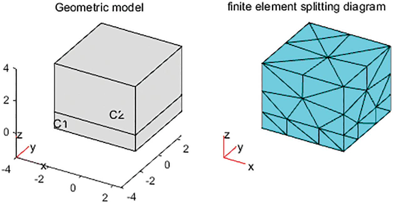
Figure 1: Geometric model and finite element splitting diagram (cubic C1 with length 50 mm, width 50 mm and height 0.1 mm, cubic C2 with length 50 mm, width 50 mm and height 1 mm)

For the steady state equation and the stochastic partial differential equation, we take Robin boundary condition. The steady state equation has no initial value, while the stochastic partial differential equation sets the initial value of the C1 module as 106, the initial value of C2 module is 0. The C1 module is considered as the radioactive source, while the C2 module is considered as the detector receiving the signal.

Take a straight line, for example, y=10z=1 and the line intersects with the finite element space to get the line segment. 40 points are randomly taken on the segment, and the numerical solution at 40 points is computed by the finite element method. According to the relevant theory [32,33], the numerical solution is unique and stable, so we can divide the geometrical model into 5381, 6732, 10,291 and 14,232 small tetrahedrons, in which the numerical simulation result of dividing the tangent into 14,232 tetrahedron is regarded as the exact solution of the corresponding position.

For stochastic partial differential equations with stochastic terms, let the time range T = 200 ps, and the time is divided into 100 parts. The calculation repeats 30 times, and the mean value of 30 numerical solutions is used to approximate the expectation of numerical solution.

Fig. 2 shows the distribution of the numerical solution of the stochastic partial differential equation model and the steady state model.

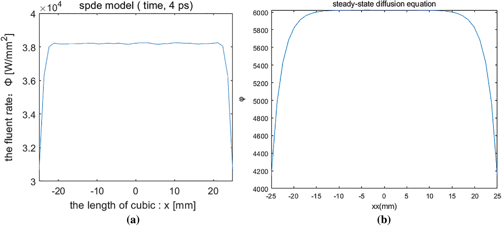
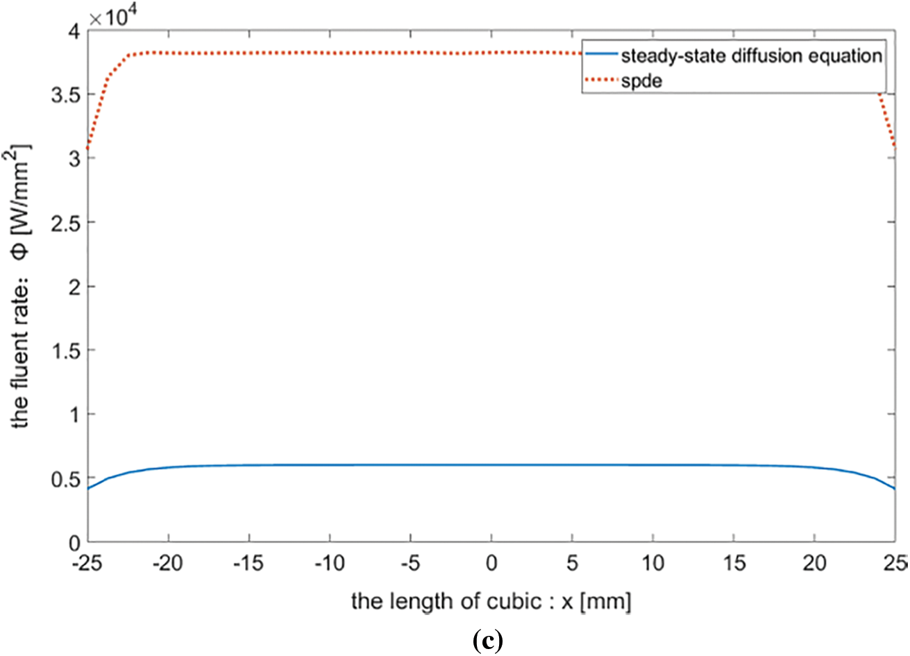
Figure 2: (a) Numerical solution of stochastic partial differential equation (b) Numerical solution of steady-state diffusion equation (c) Comparison of numerical solutions

With t = 4 ps, the distribution of the numerical solution of the stochastic partial differential equation on the line is shown in Fig. 2a. The numerical solution of the steady-state equation on the line segment is distributed as Fig. 2b. Fig. 2c shows the comparison of the two, it is known that the solution of the stochastic partial differential is greater than the solution is given by the steady-state model at the time of 4 ps. The solutions of the SPDE and the steady-state diffusion equation are rapidly decreasing at the boundary and relatively homogeneous in the interior.

Table 1 is a relative error analysis table for stochastic partial differential equations and steady-state diffusion equations under different cutting precision of finite element. From the above experimental data, we can see that the numerical simulation solution of the stochastic partial differential equation is different from the numerical simulation solution of the steady-state diffusion equation. For the stochastic partial differential equation, with the gradual increase of the split, the numerical errors obtained by the experiment are more and more small, and the steady state equation is more accurate than the stochastic parabolic equation under the same finite element segmentation precision. Compared with the steady-state diffusion equation, because the photon flow rate Φ is a stochastic process, it is reasonable to believe that the numerical solution precision of the SPDE can be improved if the number of repeated tests is further increased. In addition, finer spatial partitions, smaller time intervals, will help improve the accuracy of numerical solutions.

The next step is to study the relation between the Cherenkov imaging process of the stochastic partial differential equation and Monte Carlo simulation.

3.3 Monte Carlo Simulation of Cherenkov Imaging Process

In order to compare the effect of the stochastic partial differential equation and the steady-state diffusion equation on the Cherenkov imaging process, simulation software is an economical solution. There is a large amount of Monte Carlo simulation packages available. Among these codes, GEANT4 is the most commonly used option for Cherenkov, partly because of its flexibility in the description of complex detectors and its accurate physics models. For the research of Cherenkov, GEANT4 can simulate the physical process of photon and charged particles in matter, and GEANT4 has reliable electromagnetic physical model and flexible detector design, which is the most preferred simulation tool [37,38]. In this paper we focus on the Cherenkov effect of optical transmission simulation.

Glaster et al. [37] run the Monte Carlo simulations using the GEANT4 Architecture for Medically- oriented Simulations (GAMOS) tissue-optics plug-in. They simulated ten radionuclides including18 F, which induced Cherenkov radiation. And they drew the figures which showed the measurement results and the Monte Carlo simulations.

On this basis, we designed the following geometric model (Fig. 3) to compare the numerical solution and the GEANT4 simulations. A 50mm3×50mm3×1mm3 homogenous domain with 18 F decay nuclide radioactive point source located at one side of the domain was generated, randomly emitting β particles at the number of 107. The particle energy is set to 500 keV, β particles in the muscle tissue produced Cherenkov. The cuboid is thought to simulate a muscle with a refractive index of n = 1.33, Photon in the transport process will also be in the cuboid simulation of the muscle tissue scattering, Rayleigh scattering, and other phenomena. The opposite side of the radiation source is split into 1mm2×1mm2 detector that detects the number of photons and the energy that are being worn out.

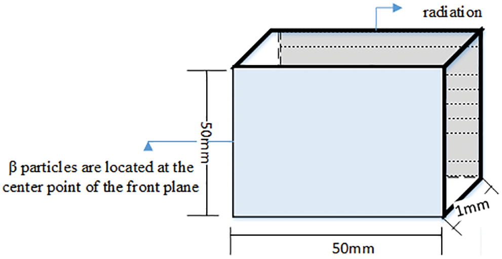
Figure 3: Geometric model

The distance between the detector and the radiation source is 1 mm because the Cherenkov photon number decreases significantly with the increase of the depth. Fig. 4 shows the attenuation diagram of photon number in the process of Cherenkov. It is known from the graph that, the number of photons absorbed increases exponentially with time. At the time of 100 ps, it decays to about 20% of the original. Fig. 5 is the relationship between photon number and position. Fig. 6 is the stereo distribution of the photon number of the detector plane, and it can be seen from the graph that the Cherenkov imaging is the point source imaging.

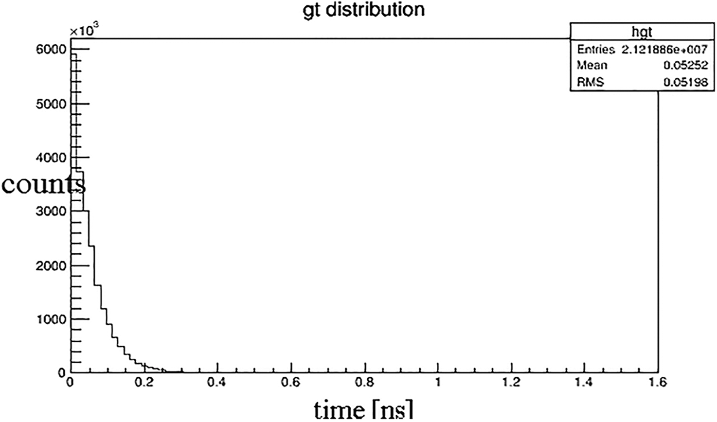
Figure 4: The relationship of photon number over time (Time unit: ns)

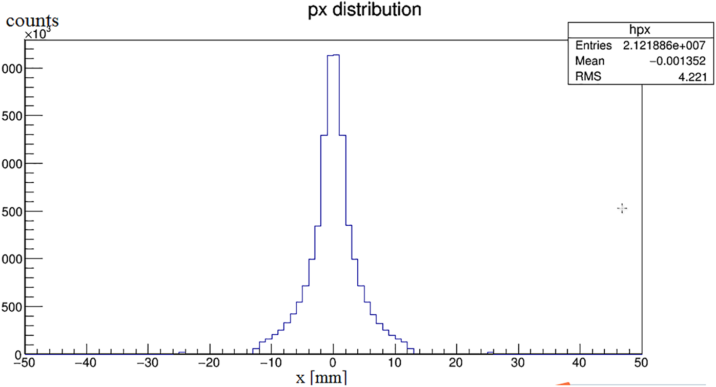
Figure 5: The relationship between photon number and position coordinates

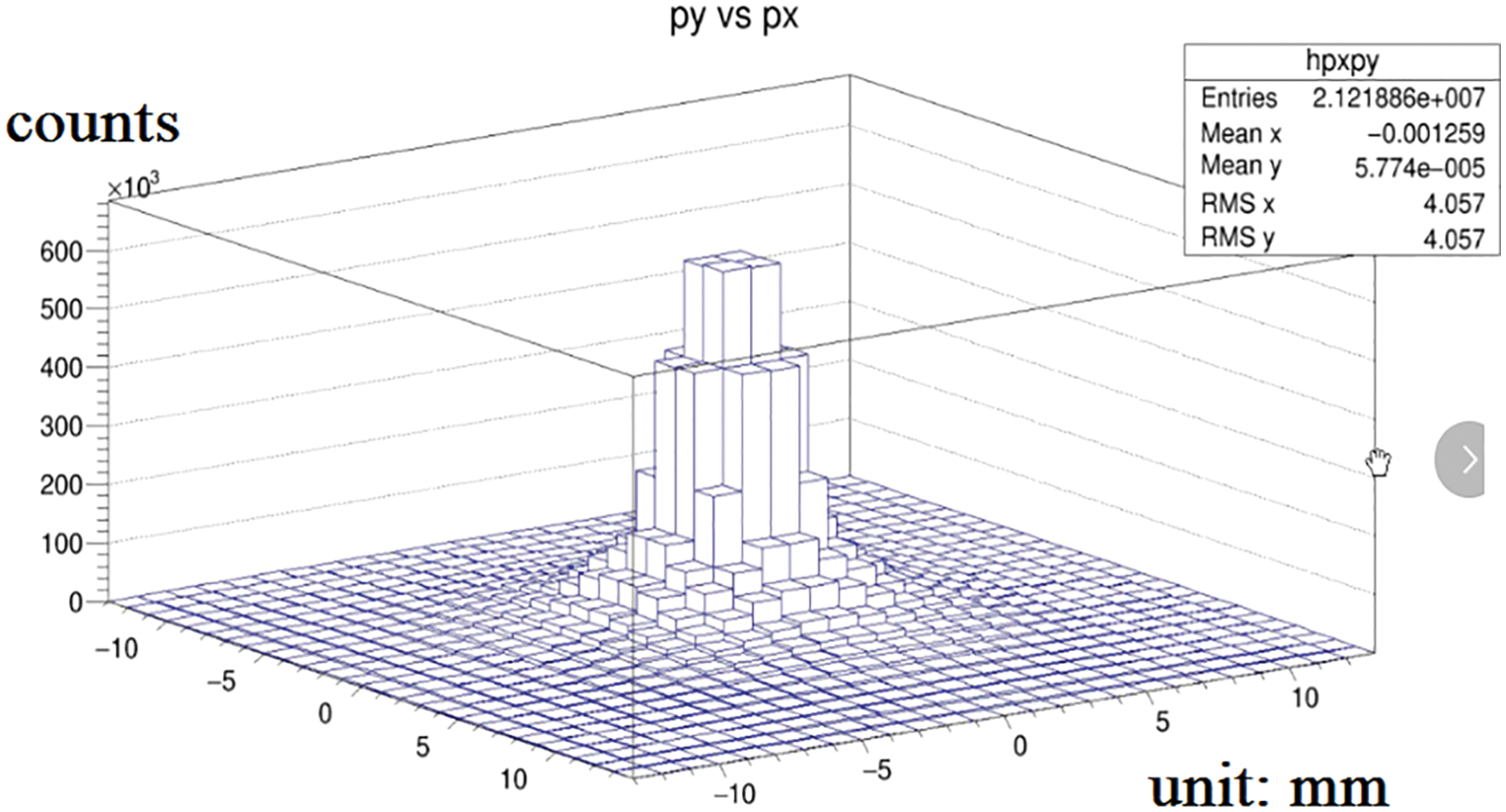
Figure 6: Three-dimensional distribution diagram of photon number

Cherenkov spectrum is a special kind of continuous spectrum of visible light, the wavelength range between 300–750 nm. In the GEANT4 simulation, the initial numbers of β particle were set to 107, so the initial energy was calculated to be about 1.66×106∼4.14×106eV. So, the initial value of the stochastic partial differential equation is set to 4×106eV/ns. According to the transport equation theory, the detector receives the photon flow rate of the boundary ∂Ω. Let’s take a point randomly, for example, (2,10,1), the outgoing photon energy numerical solution of the point is obtained by using the finite element method to solve the stochastic partial differential equation, and then the photon flow rate of the point is obtained by the formula

−D(r)(ν⋅∇Φ(r,t))=Φ(r,t)/(2U)(15)

It is also known from Section 3.3 that, at the same moment, the photon flow rate is basically uniform distribution at the different positions near the center, and each small detector has a 1 mm2 area, which can be used to calculate the curve of energy changing with time at any detector. A curve in which the energy of the detector received by the GEANT4 Simulation (2,10,1) is changed over time. The results obtained from the GEANT4 simulation are compared with those of the numerical solution of the diffusion theory in the form of stochastic partial differential equations (Fig. 7).

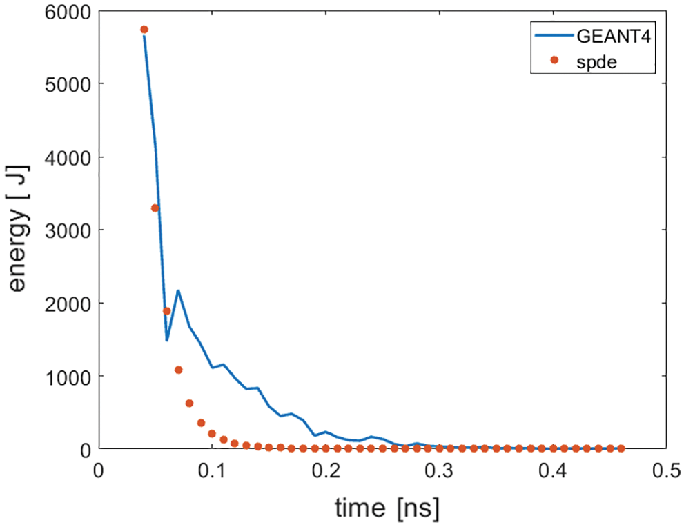
Figure 7: The temporal fluence for a homogenous cubic medium in comparison to the SPDE

4  Discussion

In this study, we propose and study the numerical solution of the stochastic partial differential, based on the GEANT4 simulation of the Cherenkov of 18 F radioisotope in muscle. The study shows that the form of stochastic partial differential equation is more helpful to simulate the radiation-induced optical transmission in biological media.

It is known from Section 3.4 that the numerical solution of the SPDE has a high degree of coincidence with the photon attenuation process obtained by the GEANT4 simulation. In Fig. 7, when t in 0.5~0.8 ns, the error is caused by a sudden increase in energy due to random selection. In addition, output rate of Cherenkov is low, and the attenuation is serious, which seriously affects the quality of Cherenkov biological imaging. It is known from Section 3.3 that the numerical solution of the stochastic partial differential equation and the common steady-state diffusion equation are inferior to one order of magnitude. In this paper, the numerical solution of the stochastic partial differential equation is larger, and the problem of poor Cherenkov imaging quality may be alleviated to some extent. The results obtained from the GEANT4 simulation are compared with those of the numerical solution of the diffusion theory in the form of stochastic partial differential equations (Fig. 7). This study shows that the form of stochastic partial differential equation is more helpful to simulate the radiation-induced optical transmission in biological media.

5  Conclusion

When the time resolution is high enough, the numerical solution of the stochastic diffusion equation is better than the numerical solution of the steady-state diffusion equation, which may provide a new way to alleviate the problem of Cherenkov luminescent imaging quality. This study shows that the form of stochastic partial differential equation is more helpful to simulate the radiation-induced optical transmission in biological media.

Acknowledgement: We would like to thank the reviewer for the many useful comments.

Authors’ Contributions:QL was a major contributor in the GEANT4 simulation. ZD advanced stochastic models and algorithms, and was a major contributor in writing the manuscript. DY was a major contributor in the error estimates. All authors read and approved the final manuscript.

Funding Statement:National Science Foundation of China (NSFC) (61671009, 12171178).

Conflicts of Interest: The authors declare that they have no conflicts of interest to report regarding the present study.

References

1. Weissleder, R. (1999). Molecular imaging: Exploring the next frontier. Radiology, 212(3), 609–614. [Google Scholar]
2. Blankenberg, F. G. (2004). Molecular imaging with single photon emission computed tomography. IEEE Engineering in Medicine and Biology Magazine, 23(4), 51–57. [Google Scholar]
3. Nienhaus, G. U., Wiedenmann, J. (2010). Structure, dynamics and optical properties of fluorescent proteins: Perspectives for marker development. Chemphyschem, 10(9–10), 1369–1379. [Google Scholar]
4. Baker, M. (2010). Nanotechnology imaging probes: Smaller and more stable. Nature Methods, 7(12), 957–962. [Google Scholar]
5. Cherenkov, P. A. (1934). Visible emission of clean liquids by action of γ radiation. Doklady Akademii Nauk Sssr, 2, 451–454. [Google Scholar]
6. Jeong, S. Y., Hwang, M. H., Kim, J. E., Kang, S., Park, J. C. (2011). Combined cerenkov luminescence and nuclear imaging of radioiodine in the thyroid gland and thyroid cancer cells expressing sodium iodide symporter: Initial feasibility study. Endocrine Journal, 58(7), 575–583. DOI 10.1507/endocrj.K11E-051. [Google Scholar] [CrossRef]
7. Robertson, R., Germanos, M. S., Manfredi, M. G., Smith, P. G., Silva, M. D. (2011). Multimodal imaging with (18)F-FDG PET and cerenkov luminescence imaging after MLN4924 treatment in a human lymphoma xenograft model. Journal of Nuclear Medicine Official Publication Society of Nuclear Medicine, 52(11), 1764–1769. [Google Scholar]
8. Jelley, J. V. (1955). Special article: Cerenkov radiation and its applications. British Journal of Applied Physics, 6(7), 227–232. DOI 10.1088/0508-3443/6/7/301. [Google Scholar] [CrossRef]
9. Ishimaru, A. (1989). Diffusion of light in turbid material. Applied Optics, 28(12), 2210–2215. DOI 10.1364/AO.28.002210. [Google Scholar] [CrossRef]
10. Gibson, A. P., Hebden, J. C., Arridge, S. R. (2005). Recent advances in diffuse optical imaging. Physics in Medicine and Biology, 50(4), 1–43. DOI 10.1088/0031-9155/50/4/R01. [Google Scholar] [CrossRef]
11. Spinelli, A. E., Kuo, C., Rice, B. W., Calandrino, R., Marzola, P. (2011). Multispectral cerenkov luminescence tomography for small animal optical imaging. Optics Express, 19(13), 12605–12618. DOI 10.1364/OE.19.012605. [Google Scholar] [CrossRef]
12. Li, C., Mitchell, G. S., Cherry, S. R. (2010). Cerenkov luminescence tomography for small animal imaging. Optics Letters, 35(7), 1109–1111. DOI 10.1364/OL.35.001109. [Google Scholar] [CrossRef]
13. Wang, G., Li, Y., Jiang, M. (2004). Uniqueness theorems in bioluminescence tomography. Medical Physics, 31(8), 2289–2299. DOI 10.1118/1.1766420. [Google Scholar] [CrossRef]
14. Zhong, J., Tian, J., Yang, X., Qin, C. (2011). Whole-body cerenkov luminescence tomography with the finite element SP3 method. Annals of Biomedical Engineering, 39(6), 1728–1735. DOI 10.1007/s10439-011-0261-1. [Google Scholar] [CrossRef]
15. Jelley, J. V. (1955). Cerenkov radiation and its applications. British Journal of Applied Physics, 6(7), 227–232. DOI 10.1088/0508-3443/6/7/301. [Google Scholar] [CrossRef]
16. Henry, A. F., Scott, C. C., Moorthy, S. (1977). Nuclear reactor analysis. IEEE Transactions on Nuclear Science, 24(6), 2367–2566. DOI 10.1109/TNS.1977.4329257. [Google Scholar] [CrossRef]
17. Ishimaru, A. (1978). Wave propagation and scattering in random media, vol. 2. New York: Academic Press. [Google Scholar]
18. Ntziachristos, V., Ripoll, J., Wang, L. V., Weissleder, R. (2005). Looking and listening to light: The evolution of whole-body photonic imaging. Nature Biotechnology, 23(3), 313–320. DOI 10.1038/nbt1074. [Google Scholar] [CrossRef]
19. Dogdas, B., Stout, D., Chatziioannou, A. F., Leahy, R. M. (2007). Digimouse: A 3D whole body mouse atlas from CT and cryosection data. Physics in Medicine & Biology, 52(3), 577–587. DOI 10.1088/0031-9155/52/3/003. [Google Scholar] [CrossRef]
20. Hielscher, A. H., Klose, A. D., Schee, A. K., Moaanderson, I. B., Backhaus, M. (2004). Sagittal laser optical tomography for imaging of rheumatoid finger joints. Physics in Medicine & Biology, 49(7), 1147–1163. DOI 10.1088/0031-9155/49/7/005. [Google Scholar] [CrossRef]
21. Klose, A. D. (2007). Transport-theory-based stochastic image reconstruction of bioluminescent sources. Journal of the Optical Society of America A: Optics Image Science and Vision, 24(6), 1601–1608. DOI 10.1364/JOSAA.24.001601. [Google Scholar] [CrossRef]
22. Losada, J., Nieto, J. J. (2021). Fractional integral associated to fractional derivatives with nonsingular kernels. Progress in Fractional Differentiation and Applications, 7(3), 137–143. DOI 10.18576/pfda/070301. [Google Scholar] [CrossRef]
23. Al-Refai, M. (2020). Maximum principles for nonlinear fractional differential equations in reliable space. Progress in Fractional Differentiation and Applications, 6(2), 95–99. DOI 10.18576/pfda/060202. [Google Scholar] [CrossRef]
24. Caputo, M., Fabrizio, M. (2021). On the singular kernels for fractional derivatives: Some applications to partial differential equations. Progress in Fractional Differentiation and Applications, 7(2), 79–82. DOI 10.18576/pfda/070201. [Google Scholar] [CrossRef]
25. Veeresha, P., Baskonus, H. M., Gao, W. (2021). Strong interacting internal waves in rotating ocean: Novel fractional approach. Axioms, 10(2), 123. [Google Scholar]
26. Ilhan, E., Veeresha, P., Baskonus, H. M. (2021). Fractional approach for a mathematical model of atmospheric dynamics of CO2 gas with an efficient method. Chaos, Solitons and Fractals, 152(4), 111–347. DOI 10.1016/j.chaos.2021.111347. [Google Scholar] [CrossRef]
27. Ross, S. M. (1983). Stochastic processes. John Wiley & Sons. [Google Scholar]
28. Ito, K. (1946). On a stochastic integral equation. Proceedings of the Japan Academy, 22(1–4), 32–35. DOI 10.2183/pjab1945.22.32. [Google Scholar] [CrossRef]
29. Ito, K. (1951). On stochastic differential equations, vol. 4. American Mathematical Society. DOI 10.1090/memo/0004. [Google Scholar] [CrossRef]
30. Prato, G. D., Zabczyk, J. (1992). Stochastic equations in infinite dimensions. Cambridge University Press. [Google Scholar]
31. Yan, Y. (2004). Galerkin finite element methods for stochastic parabolic partial differential equations. Siam Journal on Numerical Analysis, 43(4), 1363–1384. DOI 10.1137/040605278. [Google Scholar] [CrossRef]
32. Walsh, J. B. (2005). Finite element methods for parabolic stochastic PDEs. Potential Analysis, 23(1), 1–43. DOI 10.1007/s11118-004-2950-y. [Google Scholar] [CrossRef]
33. Kossioris, G. T., Zouraris, G. E. (2009). Fully-discrete finite element approximations for a fourth-order linear stochastic parabolic equation with additive space-time white noise: II. 2D and 3D case. Mathematics, 44(2), 289–322. [Google Scholar]
34. Jentzen, A., Roeckner, M. (2010). A break of the complexity of the numerical approximation of nonlinear SPDEs with multiplicative noise. Agricultural & Forest Entomology, 2, 161–166. [Google Scholar]
35. Han, R., Liang, J., Qu, X., Hou, Y., Ren, N. (2009). A source reconstruction algorithm based on adaptive hp-FEM for bioluminescence tomography. Optics Express, 17(17), 14481–14494. DOI 10.1364/OE.17.014481. [Google Scholar] [CrossRef]
36. Allen, E. J., Novosel, S. J., Zhang, Z. (1998). Finite element and difference approximation of some linear stochastic partial differential equations. Stochastics and Stochastic Reports, 64(1–2), 117–142. DOI 10.1080/17442509808834159. [Google Scholar] [CrossRef]
37. Glaster, A. K., Andreozzi, J. M., Gladstone, D. J., Pogue, B. W. (2015). Cherenkov radiation fluence estimates in tissue for molecular imaging and therapy applications. Physics in Medicine & Biology, 60(17), 6701–6718. DOI 10.1088/0031-9155/60/17/6701. [Google Scholar] [CrossRef]
38. Gillam, J. E., Rafecas, M. (2016). Monte-Carlo simulations and image reconstruction for novel imaging scenarios in emission tomography. Nuclear Instruments and Methods in Physics Research Section A: Accelerators, Spectrometers, Detectors and Associated Equipment, 809(7), 76–88. DOI 10.1016/j.nima.2015.09.084. [Google Scholar] [CrossRef]
Cite This Article
Copyright © 2023 The Author(s). Published by Tech Science Press.
This work is licensed under a Creative Commons Attribution 4.0 International License , which permits unrestricted use, distribution, and reproduction in any medium, provided the original work is properly cited.
Downloads
Citation Tools