A Modified Formulation of Singular Boundary Method for Exterior Acoustics

1  Introduction

As we all know, the main numerical methods to study acoustic radiation and scattering are the finite element method (FEM) [1–4] and the boundary element method (BEM) [5–7]. The FEM is a general method for solving mathematical and physical equations. However, the FEM is difficult in dealing with the infinite domain problems and needs several additional technologies [8–10]. The BEM is a boundary-type numerical algorithm after the FEM. The fundamental solutions of the BEM can automatically satisfy the Sommerfeld radiation condition at infinity, so the BEM can effectively deal with infinite domain problems. Moreover, the BEM only needs the boundary discretization on the surface of the considered computational domains, so that it can save the computational resources. Therefore, the BEM is a competitive option for infinite domain problems. However, the fundamental solution of the BEM has singularities, which leads to a great deal of difficulty in the calculation of the singular/hypersingular integrals. This is also the main factor limiting the application of BEM.

To avoid these troublesome calculations in the BEM, the method of fundamental solutions (MFS) [11–16] was proposed. It distributes the source points outside the solution domain to overcome the singularities of the fundamental solutions, which is effective and easy to implement. However, the optimal placement of the source points is a nontrivial task, which has a big effect on the numerical stability and accuracy in the MFS, in particular the problems with multi-connected domains or complicated-geometric-shaped domains.

Then the boundary knot method (BKM) [17–19] has been proposed, which employs the nonsingular general solutions as basis functions instead of the singular fundamental solutions. It avoids the troublesome placement of the source points in the MFS. However, it cannot be used for exterior Helmholtz problems due to the nontrivial task of the derivation of the nonsingular general solutions. To overcome this drawback, several numerical methods have been proposed to solve acoustic radiation and scattering problems in recent years, such as the singular boundary method (SBM) [20–24], the regularized meshless method (RMM) [25,26], and so on. Here we focus on the singular boundary method (SBM).

The SBM introduces the concept of origin intensity factor (OIF) [27] to substitute the singular term in the interpolation expression, so that we can obtain the non-singular interpolation expression. In order to determine the OIF, the SBM uses the inverse interpolation technique (IIT) [28], which needs to construct the sample solution and select the sample nodes in the physical domain. However, the accuracy of numerical results will be affected sensitively by the selection of sample points, which limits the application of the method in three-dimensional problems. The improved formulation of the singular boundary method is proposed by Chen and his coworkers [29–32] to overcome this issue. The method derives the origin intensity factor through the subtracting and adding-back technique, so as to avoid the selection of sample nodes in the SBM.

Although the improved formulation of the SBM has been applied to the acoustic wave propagation problems [33–35], it still cannot obtain the correct numerical results in the solution of the acoustic radiation and scattering problems in the infinite domain, which is caused by the non-uniqueness issue appeared near the corresponding internal characteristic frequencies. The combined Helmholtz integral equation formulation (CHIEF) method [36–38] and the Burton-Miller formulation [7,21] are two popular schemes to avoid this non-uniqueness issue. However, the CHIEF method can only avoid the uniqueness issue at some but not all characteristic frequencies. And the Burton-Miller formulation is usually difficult to calculate due to the existence of singularities and hyper-singularities in fundamental solutions. Inspire by Chen’s work [39] in indirect BEM, this study constructs a modified formulation of the SBM based on CHIEF method and self-regularization technique to deal with this non-uniqueness issue.

This paper presents a modified formulation of the SBM in conjunction with the CHIEF method and self-regularization technique to exterior acoustics analysis. The paper is briefly summarized as follows: Section 2 introduces the modified formulation of the SBM in conjunction with the CHIEF method and self-regularization technique. Section 3 verifies the accuracy of the proposed method and compared the present solutions with the analytical solutions and the solutions of other methods through several typical benchmark examples. Finally, Section 4 presents some conclusions of the study.

2  Methodology

Considering the propagation of time-harmonic acoustic waves in a homogeneous isotropic, the acoustic radiation and scattering can be described by the Helmholtz equation

(Δ+k2)u(x)=0,x∈D(1)

and the boundary conditions

u(x)=u¯,x∈ΓD(2)

q(x)=∂u(x)∂nx=q¯,x∈ΓN(3)

where D is the exterior domain, k=ωc stands for the wave number, in which c denotes the sound velocity, ω presents the angular frequency. Respectively, ΓD and ΓN represent the Dirichlet boundary and Neumann boundary. For different types of the acoustics problems, the acoustic pressure u(x) can be expressed as

u={uR=uT,if only radiationus=uT−uinc,if only scatteringuR+S=uT−uinc,if both(4)

where the subscripts T, R, S, inc represent the total, radiation, scattering and incidence wave, respectively. For the physical and mechanical problems, it is required to impose the well-known Sommerfeld radiation condition on the infinite boundary conditions

limr→∞r12(n−1)(∂u∂r−iku)=0(5)

where n stands for the dimension of the problem and i=−1 .

2.1 Original Singular Boundary Method (SBM)

Considering the Helmholtz equation with infinite domain, the single-layer fundamental solution is used as the interpolation basic function in the SBM. The approximate solutions u(x) and q(x) can be expressed as

u(xm)={∑j=1NajϕFH(xm,sj),xm∈D∑j=1j≠mNajϕFH(xm,sj)+amUSjj,xm∈ΓD(6)

q(xm)=∂u(xm)∂nx={∑j=1Naj∂ϕFH(xm,sj)∂nx,xm∈D∑j=1j≠mNaj∂ϕFH(xm,sj)∂nx+amQSjj,xm∈ΓN(7)

where aj stands for the unknown coefficient, {xm} denotes the collocation points, {sj} is the source points, N represents the number of source points {sj}, nx stands for the outward unit normal vector on the collocation points {xm}, USjj and QSjj represent the OIFs. The fundamental solutions ϕFH(xm,sj)={i4H0(1)(krmj),2Dcaseeikrmj4πrmj,3Dcase, where Hn(1) denotes nth order Hankel function of the first kind, rmj=‖xm−sj‖2 is the Euclidean distance. When the collocation point xm coincides with the source point sj, the fundamental solution ϕFH(xm,sj) has singularities. Here the OIFs are introduced to replace the singular terms. By considering the same singularity between the Helmholtz fundamental solutions and Laplace fundamental solutions, the explicit relationship between the OIFs for Laplace equation and Helmholtz equation is derived. Therefore the key issue in the acoustic SBM is to determine the OIFs (U0jj and Q0jj) of Laplace equations. Then the corresponding OIFs U0jj and Q0jj can be determined by using the subtracting and adding-back technique, which can be represented as follows [32]:

U0jj={−ln⁡(Lj/2π)2π,2Dcase−∑j=1,j≠mJLjLm[ϕFL(xm,sj)qSL(sj)−∂ϕFL(xm,sj)∂nsuSL(sj)],3Dcase(8)

Q0jj=−1Lm−∑j=1j≠mNLjLm∂ϕFL(xm,sj)∂ns(9)

where Lm is the influence area of mth source point, uSL(sj)=⟨sj−xm,nxm⟩ and qSL(sj)=∂uSL(sj)∂nsj=⟨nsj,nxm⟩ denotes the specific sample solutions, in which ⟨vec1,vec2⟩ stands for the dot product of two vectors, vec1 and vec2. Fig. 1 shows the schematic configuration of the source points and their infinitesimal areas Lj. More detailed derivation can be found in the literature [32].

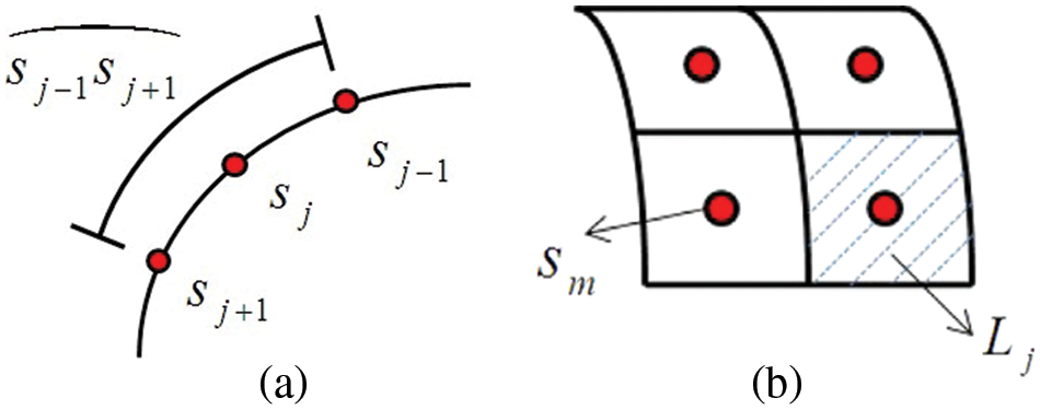
Figure 1: Schematic configuration of the source points sj (a) the curve sj−1sj+1 on 2D problems, (b) the corresponding infinitesimal area Lj on 3D problems

Then the corresponding OIFs USjj and QSjj can be represented as follows:

USjj=U0jj+B,(10)

QSjj=Q0jj=−1Lm−∑j=1j≠mNLjLm∂ϕFL(xm,sj)∂ns(11)

where the complex number B=−12π[ln⁡(k2)+γ−iπ2] in 2D problems and B=ik4π in 3D problems.

Taking the collocation points and the source points as the same set of boundary points, the following matrix form can be obtained by substituting Eqs. (6) and (7) into Eqs. (1)–(3),

AN×NaN×1=bN×1(12)

in which

A=[A1A2],b=[b1b2]

A1=(A1)mj,m=1,⋯,N1;j=1,⋯,N

A2=(A2)mj,m=N1+1,⋯,N;j=1,⋯,N

(A1)mj=ϕFH(xm,sj),m≠j,(A1)mj=USjj,m=j

(A2)mj=∂ϕFH(xm,sj)∂nx,m≠j,(A1)mj=QSjj,m=j

b1=[u¯(x1),⋯,u¯(xN1)]T

b2=[q¯(xN1+1),⋯,q¯(xN)]T

By solving Eq. (12), the unknown coefficients a={aj} can be determined. After that, the numerical acoustic pressure u(x) inside the domain and on the boundary can be calculated by using the SBM formulation (6).

2.2 The SBM Coupled with the CHIEF Method and Self-Regularization Technique (SR-CHIEF-SBM)

In the SBM solution of exterior acoustic problems, the resultant matrix is rank deficient when the wave frequency is exactly equal to the eigenfrequency of the corresponding interior acoustic problems, which makes the original SBM unable to obtain the correct solution. To overcome this non-uniqueness issue, it needs to introduce NC CHIEF points {xc} in the interior domain ℜ2∖D to provide NC additional independent constraint equations for generating a sufficient number of independent equations.

Based on the self-regularization technique and the singular value decomposition (SVD) technique, NC additional independent constraint equations can be represented as follows:

∑j=1N⁡ajϕSVDcH(xc,sj)=0,c=1,2,⋯,NC(13)

where ϕSVDc denotes the right unitary vectors of the right unitary matrix ΨSVD=[ϕSVDN,⋯,ϕSVD1] decomposed by using the singular value decomposition on the matrix [A]N×N=[ΨSVD]N×N[ΣSVD]N×N[ΨSVD]N×NH, in which ΣSVD=[σN⋯0⋮⋱⋮0⋯σ1] with the singular values σN≥σN−1≥⋯≥σ1, the superscript H denotes the Hermitian transpose. The SBM formulations (6) and (7) coupled with Eq. (13) are abbreviated as CHIEF-SBM in this study. The following matrix form of the CHIEF-SBM can be obtained by substituting Eqs. (6) and (7) into Eqs. (1)–(3),

[A N×NΦ¯NC×N]aN×1=[bN×10NC×1](14)

where Φ¯NC×N=[ϕSVD1H⋯ϕSVDNCH]. By solving Eq. (14), the unknown coefficients a={aj} can be determined. After that, the numerical acoustic pressure u(x) inside the domain and on the boundary can be calculated by using the SBM formulation (6).

Moreover, to improve the numerical performance, the CHIEF points can be also considered as the extra source points, namely, {s¯j}={sj}∪{xc}. The related SBM formulations (6) and (7) can be modified as follows:

u(xm)={∑j=1NajϕFH(xm,s¯j)+∑j=N+1N+NCβjϕFH(xm,s¯j),xm∈D∑j=1j≠mNajϕFH(xm,s¯j)+∑j=N+1j≠mN+NCβjϕFH(xm,s¯j)+amUSjj,xm∈ΓD(15)

q(xm)=∂u(xm)∂nx={∑j=1Naj∂ϕFH(xm,s¯j)∂nx+∑j=N+1N+NCβj∂ϕFH(xm,s¯j)∂nx,xm∈D∑j=1Naj∂ϕFH(xm,s¯j)∂nx+∑j=N+1N+NCβj∂ϕFH(xm,s¯j)∂nx+amQSjj,xm∈ΓN(16)

subjected to NC constraint conditions (13). The SBM formulations (15) and (16) coupled with Eq. (13) are abbreviated as SR-CHIEF-SBM in this study. The following matrix form of the SR-CHIEF-SBM can be obtained by substituting Eqs. (15) and (16) into Eqs. (1)–(3),

[A N×NA ¯N×NCΦ¯NC×N0NC×NC][aN×1βNC×1]=[bN×10NC×1](17)

where β={βj} stands for the strengths of the extra source points, and A¯=[A¯1A¯2], in which

A¯1=(A¯1)mj,m=1,⋯,N1;j=1,⋯,NC

A¯2=(A¯2)mj,m=N1+1,⋯,N;j=1,⋯,NC

(A¯1)mj=ϕFH(xm,xc),

(A¯2)mj=∂ϕFH(xm,xc)∂nx

By solving Eq. (17), the unknown coefficients a={aj} can be determined. After that, the numerical acoustic pressure u(x) inside the domain and on the boundary can be calculated by using the SBM formulation (15).

3  Numerical Results

In this section, several benchmark examples are presented to verify the feasibility and accuracy of the proposed SR-CHIEF-SBM in analyzing exterior acoustic radiation and scattering behavior. The present numerical solutions are compared with the analytical solutions and the ones obtained by the original SBM, the CHIEF-SBM, and the Burton-Miller SBM (BM-SBM). To measure the accuracy, the root mean square error RMSE(u) and the maximum error Merr(u) are defined as follows:

RMSE(u)=∑i=1Nt[unum(xi)−uana(xi)]2∑i=1Ntuana2(xi)(18)

Merr(u)=max1≤i≤Nt|unum(xi)−uana(xi)|(19)

where uana(xi) and unum(xi) represent the analytical solutions and numerical solutions at ith test nodexi, Nt denotes the number of total test nodes inside the domain.

Example 1: Radiation problem of a hard infinite circular cylinder (Neumann boundary condition)

Consider the acoustic radiation by a hard infinite circular cylinder. The analytical solution of the radiation field uR is

u(r,θ)=−kaH4(1)(kr)kaH3(1)(ka)−4H4(1)(ka)cos⁡(4θ)(20)

In the proposed SR-CHIEF-SBM implementation, the parameters are set as N=300 and NC=2, the location of 2 CHIEF points in polar coordinates are (0.8a,5π/18) and (0.8a,5π/9), the test points are placed on a circle with a radius of 2a, and a=1. Fig. 2 shows the convergence rates of the proposed SR-CHIEF-SBM in comparison with the original SBM, CHIEF-SBM and BM-SBM in Example 1 with ka=5. It can be found that the numerical results obtained by the proposed SR-CHIEF-SBM, CHIEF-SBM and original SBM converge to the analytical solutions with a similar rate of convergence, while the BM-SBM provides the correct numerical results with lower accuracy due to the use of the double-layer fundamental solutions.

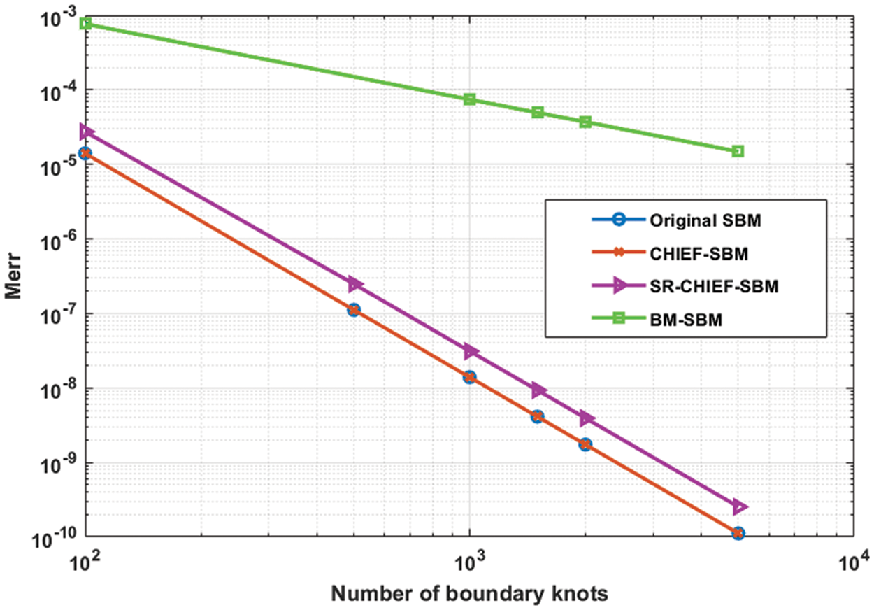
Figure 2: Convergence rates of the proposed SR-CHIEF-SBM in comparison with the original SBM, CHIEF-SBM and BM-SBM in Example 1 with ka=5

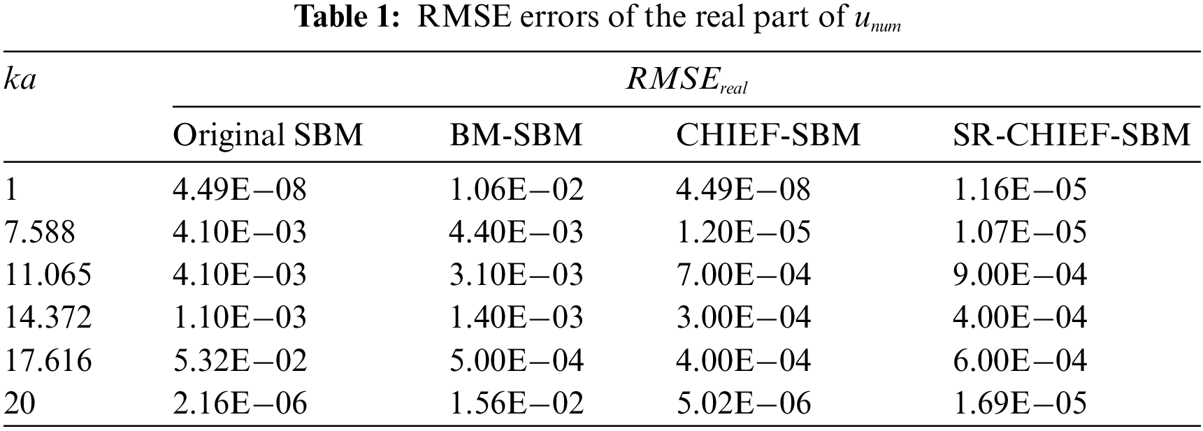
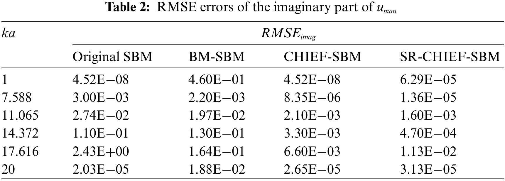
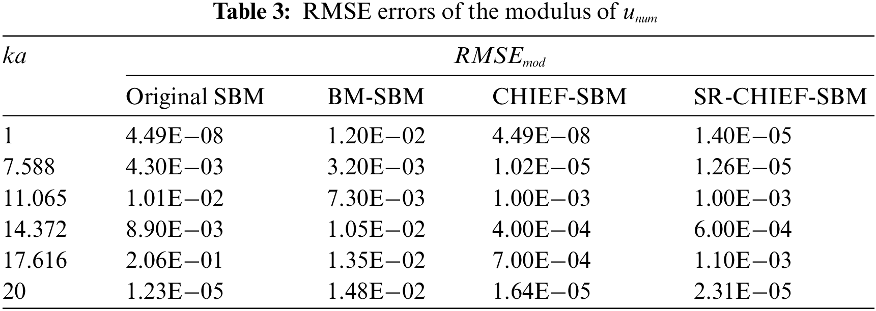
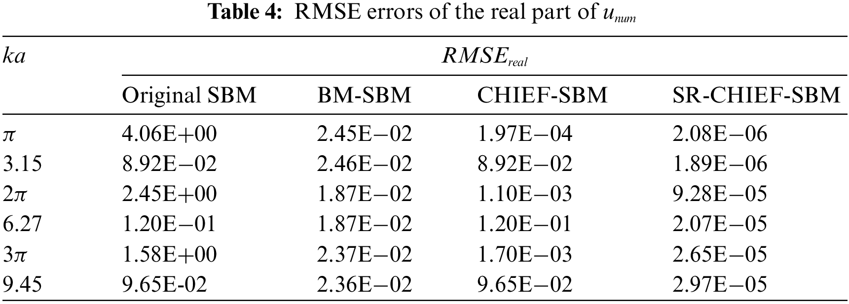
Then Tables 1–3 show the RMSE errors of the real part, imaginary part and the modulus of unum obtained by the proposed SR-CHIEF-SBM with N=300 and NC=2 in comparison with the original SBM, CHIEF-SBM and BM-SBM in Example 1. It can be found from these tables that at some specific non-dimensional wavenumbers ka=14.372,17.616, the original SBM cannot obtain the correct numerical solutions, while both the CHIEF-SBM and SR-CHIEF-SBM provide more accurate results than the BM-SBM.

Example 2: Acoustic radiation by a pulsating-sphere (Neumann boundary condition)

Next, consider acoustic radiation from a pulsating sphere as shown in Fig. 3. The sphere is applied with uniform radial velocity v0 with radius a. This model is a typical example to verify the efficiency of the numerical methods for exterior acoustics. The analytical solution of the radiation field uR is

uR(r,θ)=ar(ikaz0ika−1)v0eik(r−a)(21)

where z0=ρ0c0 stands for the characteristic impedance of the medium, ρ0 is the density of the medium and c0 represents the sound velocity.

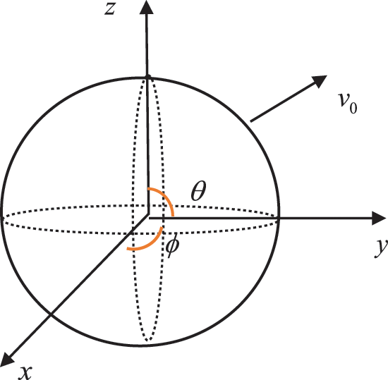
Figure 3: Sketch of the pulsating-sphere model

In the proposed SR-CHIEF-SBM implementation, the parameters are set as N=900 and NC=9, 9 CHIEF points are evenly distributed on a spherical surface with radius of 0.1, the test points are placed on a spherical surface with a radius of 2. Fig. 4 shows the convergence rates of the proposed SR-CHIEF-SBM in comparison with the original SBM, CHIEF-SBM and BM-SBM in Example 2 with ka=5. It can be found that the proposed SR-CHIEF-SBM provides the most accurate results among these four schemes. And both the CHIEF-SBM and original SBM provide accurate results with a similar rate of convergence, while the BM-SBM provides the correct numerical results with lower accuracy due to the use of the double-layer fundamental solutions.

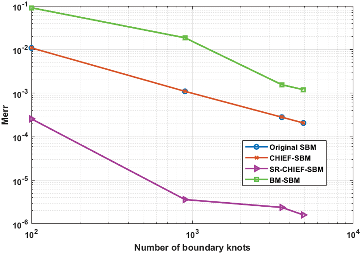
Figure 4: Convergence rates of the proposed SR-CHIEF-SBM in comparison with the original SBM, CHIEF-SBM and BM-SBM in Example 2 with ka=5

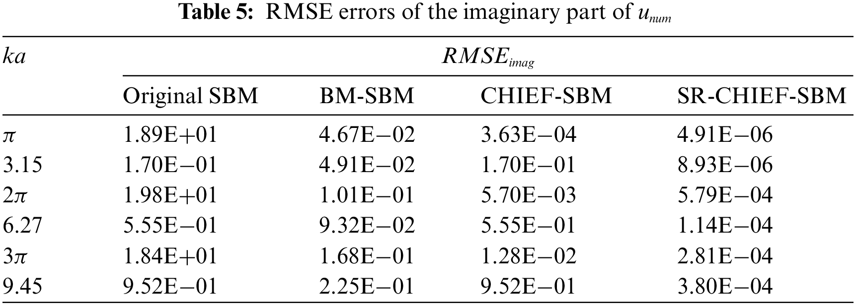
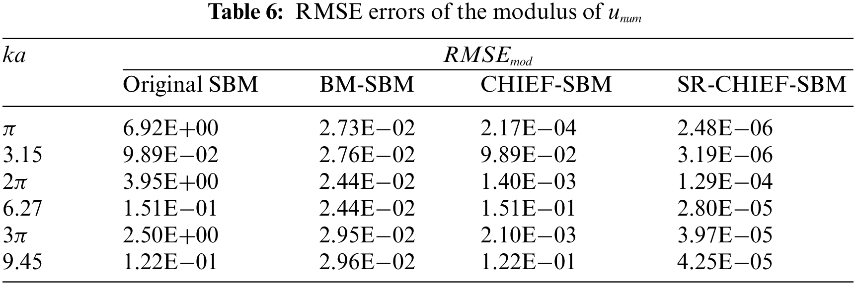
Then Tables 4–6 show the RMSE errors of the real part, imaginary part and the modulus of unum obtained by the proposed SR-CHIEF-SBM with N=900 and NC=9 in comparison with the original SBM, CHIEF-SBM and BM-SBM in Example 2. The tables show that at some specific non-dimensional wavenumbers ka=π,2π,3π, the original SBM cannot obtain the correct numerical solutions. The CHIEF-SBM can correct the numerical results at these specific non-dimensional wavenumbers, however, it may fail in the vicinity of the aforementioned specific non-dimensional wavenumbers ka=3.15,6.27,9.45. The proposed SR-CHIEF-SBM performs the accurate solutions at all these non-dimensional wavenumbers. The BM-SBM can correct the numerical solutions with lower accuracy at all these non-dimensional wavenumbers.

Example 3: Acoustic scattering by a hard sphere (Neumann boundary condition)

In this example, the scattering problem of a hard sphere subjected to an incident plane wave is considered. The incident plane wave is given as

uinc=eik[zcos⁡θ0+sin⁡θ0(xcos⁡ϕ0+ysin⁡ϕ0)](22)

where (θ0,ϕ0) denotes the angle of the incident plane wave in the spherical coordinates as shown in Fig. 5.

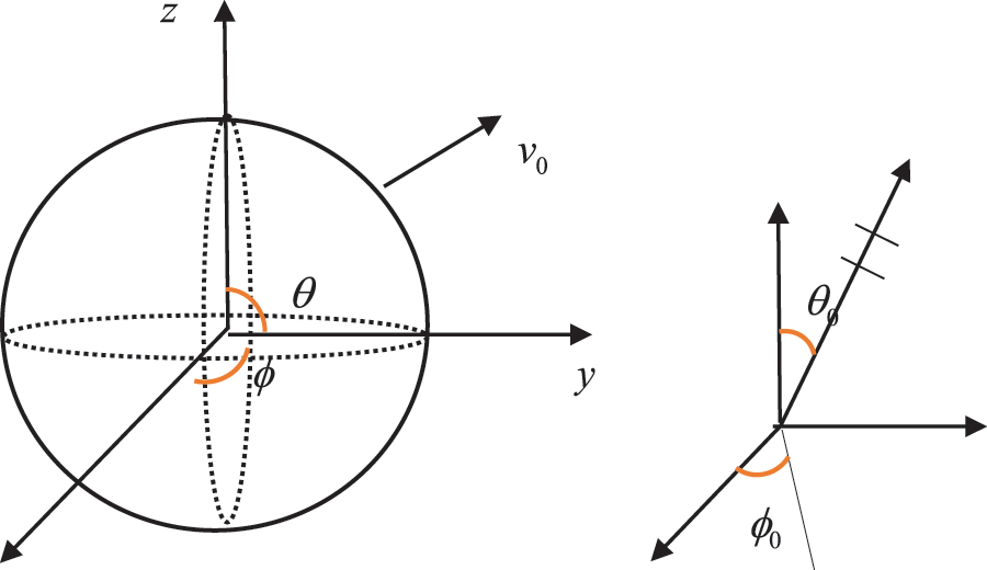
Figure 5: Sketch of the plane wave by a spherical scatter

The analytical solution of the total field is represented as

u=∑v=0∞∑w=0vivεw(2v+1)×(v−w)!(v+w)![jv(kρ)+j′(ka)hv(2)(kρ)hv′(ka)]Pvw(cos⁡θ0)Pvw(cos⁡θ)×cos⁡(wϕi)cos⁡(wϕ)(23)

In the present numerical implementation, the parameters are set as N=1600 and NC=9, 9 CHIEF points are evenly distributed on a spherical surface with a radius of 0.8. Fig. 6 shows the real part Re(u(2a,0,0)) and imaginary part Im(u(2a,0,0)) of the acoustic pressures obtained by the proposed SR-CHIEF-SBM in comparison with the original SBM, CHIEF-SBM and BM-SBM in Example 3 with the varied non-dimensional wavenumbers ka from 0.01 to 10. It can be observed that, with the increasing non-dimensional wavenumber ka, the original SBM may fail to obtain the correct numerical solutions at some specific non-dimensional wavenumbers. The BM-SBM provides the correct numerical results with lower accuracy, in particular at larger non-dimensional wavenumbers ka. Both the numerical results obtained by the CHIEF-SBM and the SR-CHIEF-SBM are in good agreement with the analytical solutions.

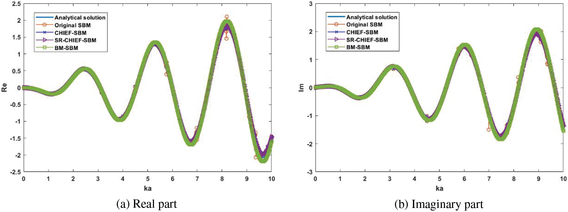
Figure 6: Frequency-sweep plot: (a) Real part of acoustic pressure Re(u(2a,0,0)), (b) Imaginary part of acoustic pressure Im(u(2a,0,0)) in Example 3

In the following examples, the normal velocity on the surface is produced by a point source of spherical dilatation wave with unit intensity located at the coordinate origin, then the related analytical radiation fields uR have the following unified formulation:

u(r,θ)=eikrr(24)

Example 4: Acoustic radiation by a hard ellipsoid (Dirichlet boundary condition)

This example considers acoustic radiation by a hard ellipsoid {(x,y,z)|x2+y2+z24≤R2} as shown in Fig. 7.

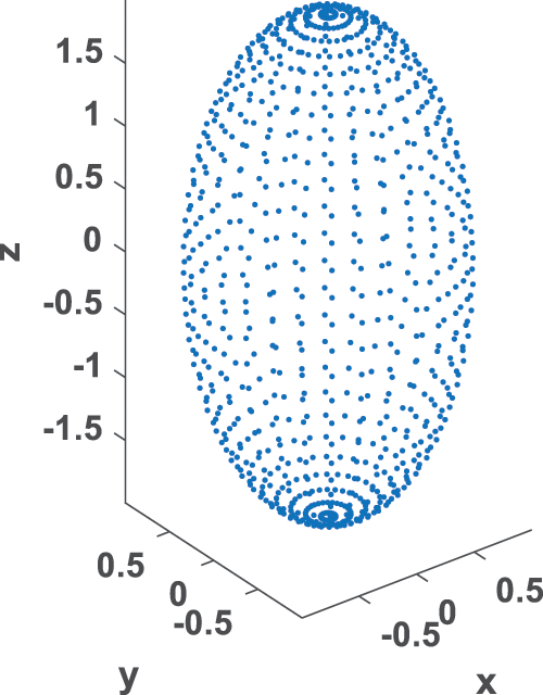
Figure 7: Sketch of wave radiation by an ellipsoid and its node distribution

In the present numerical implementation, the parameters are set as N=900 and NC=9, 9 CHIEF points are evenly distributed on a spherical surface with a radius of 0.8. Fig. 8 shows the real part Re(u(4a,0,0)) and imaginary part Im(u(4a,0,0)) of the acoustic pressures obtained by the proposed SR-CHIEF-SBM in comparison with the original SBM, CHIEF-SBM and BM-SBM in Example 4 with the varied non-dimensional wavenumbers ka from 0.01 to 10. It can be observed that, with the increasing non-dimensional wavenumber ka, the original SBM may fail to obtain the correct numerical results at some specific non-dimensional wavenumbers. The CHIEF-SBM can correct the numerical results at some small specific non-dimensional wavenumbers, however, it may still fail at some large specific non-dimensional wavenumbers. Both the numerical results obtained by the SR-CHIEF-SBM and the BM-SBM are in good agreement with the analytical solutions.

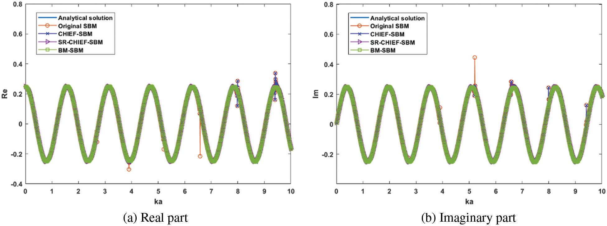
Figure 8: Frequency-sweep plot: (a) Real part of acoustic pressure Re(u(4a,0,0)), (b) Imaginary part of acoustic pressure Im(u(4a,0,0)) in Example 4

Example 5: Acoustic radiation by a microphone model (Neumann boundary condition)

Consider acoustic radiation by a microphone model. Coarse and refined node distributions are shown in Fig. 9. Here, the nodes are generated by COMSOL with coarse and refined meshes.

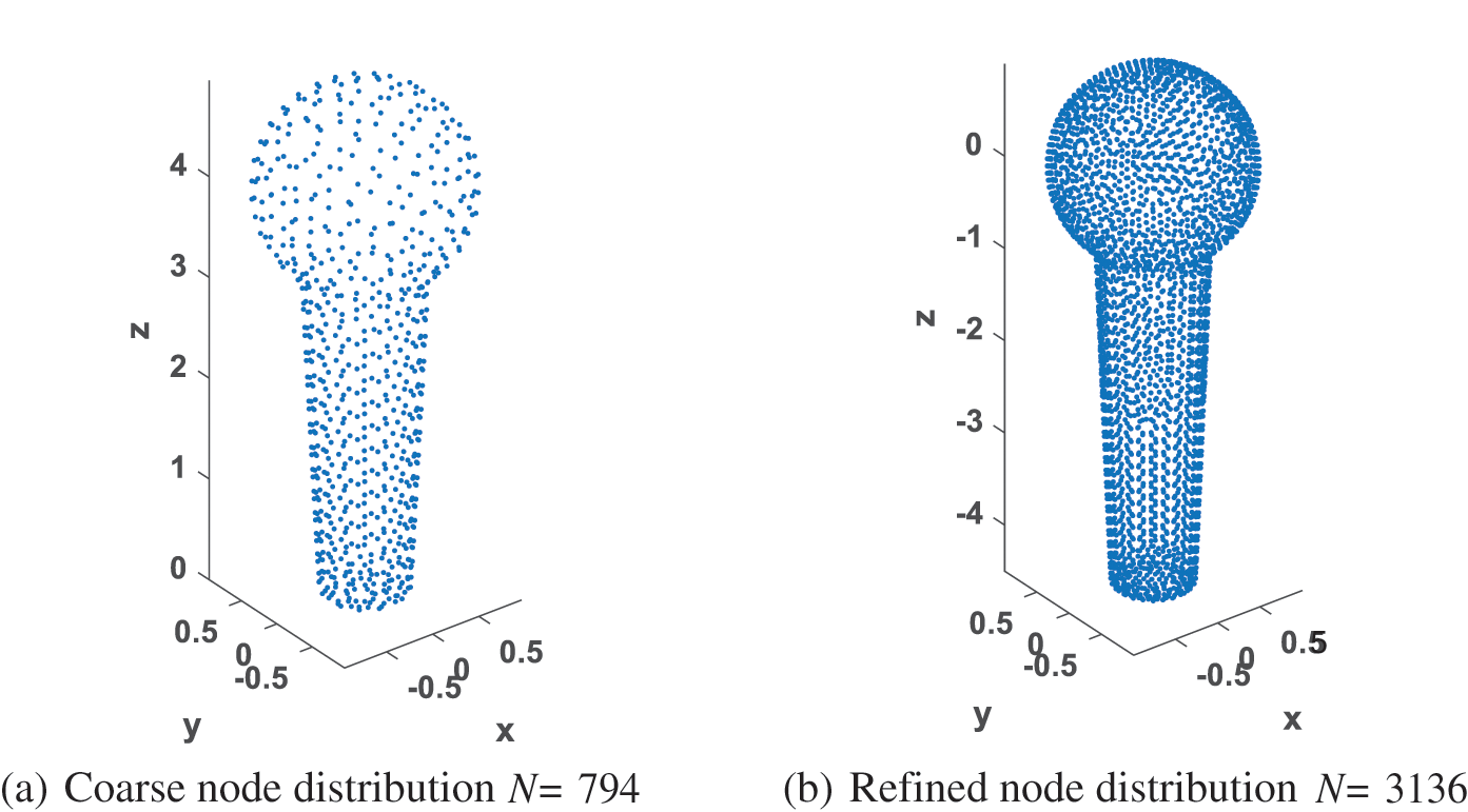
Figure 9: Sketch of wave radiation by a microphone model and its node distributions: (a) Coarse node distribution N=794, (b) Refined node distribution N=3136

In the present numerical implementation, 9 CHIEF points (NC=9) are evenly distributed on a spherical surface with a radius of 0.05, coarse node distribution N=794 is used in the SR-CHIEF-SBM, CHIEF-SBM and original SBM. It should be mentioned that the BM-SBM with coarse node distribution N=794 may fail to obtain the correct numerical results, therefore refined node distribution N=3136 is used in the BM-SBM. Fig. 10 shows the real part Re(u(0,0,2a)) and imaginary part Im(u(0,0,2a)) of the acoustic pressures obtained by the proposed SR-CHIEF-SBM (N=794) in comparison with the original SBM (N=794), CHIEF-SBM (N=794) and BM-SBM (N=3136) in Example 5 with the varied non-dimensional wavenumbers ka from 0.01 to 7. It can be observed that, with the increasing non-dimensional wavenumber ka, the original SBM may fail to obtain the correct numerical results at some specific non-dimensional wavenumbers. The CHIEF-SBM can correct the numerical solutions at these small specific non-dimensional wavenumbers, however, it may still fail at these large specific non-dimensional wavenumbers and their adjacent regions. Both the numerical results obtained by the SR-CHIEF-SBM and the BM-SBM are in good agreement with the analytical solutions, while the BM-SBM requires more refined nodes to obtain acceptable results compared with the proposed SR-CHIEF-SBM.

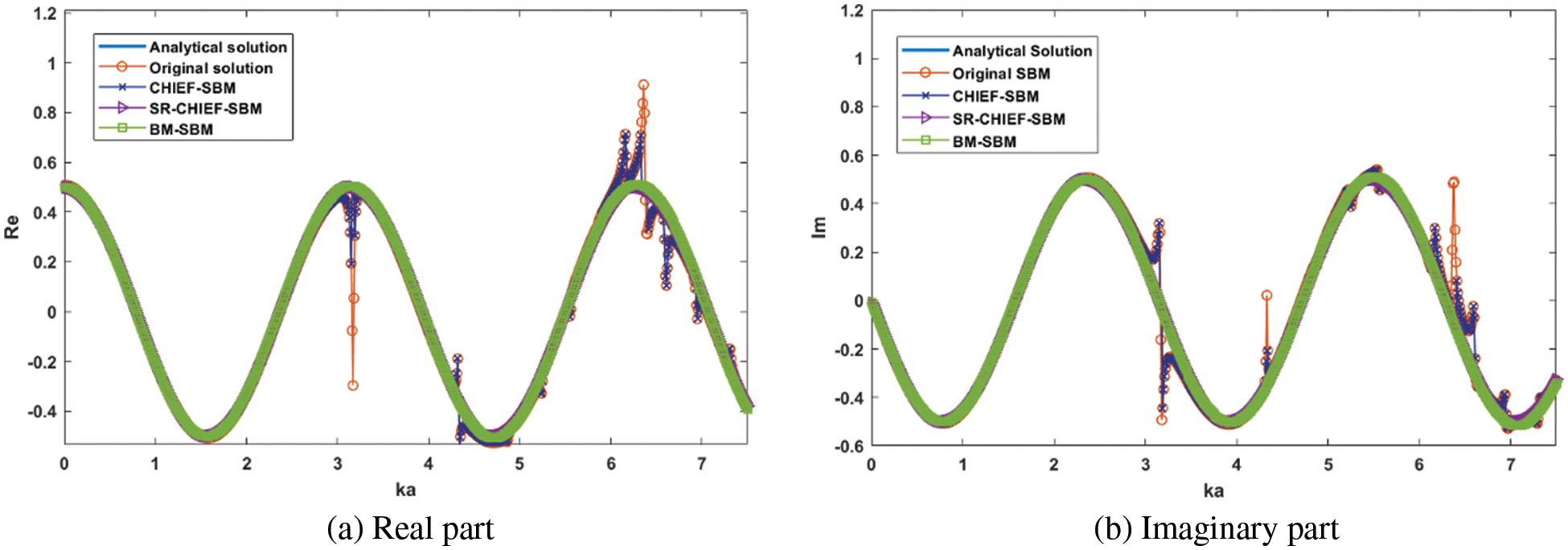
Figure 10: Frequency-sweep plot: (a) Real part of acoustic pressure Re(u(0,0,2a)), (b) Imaginary part of acoustic pressure Im(u(0,0,2a)) in Example 5

4  Conclusion

This paper proposes a modified formulation of the singular boundary method (SBM) by introducing the combined Helmholtz integral equation formulation (CHIEF) and the self-regularization technique to exterior acoustics. In the proposed scheme, the use of the CHIEF scheme and the self-regularization technique not only guarantees the unique solution of exterior acoustics, but also improves the numerical accuracy in the solution of 2D and 3D acoustic radiation and scattering problems.

Numerical investigations under several 2D and 3D benchmark examples show that the original SBM fails to obtain the correct numerical solutions at some specific non-dimensional wavenumbers related to the internal characteristic frequencies due to the non-uniqueness issue frequently encountered in the boundary discretization of exterior acoustics. The CHIEF-SBM can eliminate these non-uniqueness problems at the relatively small specific non-dimensional wavenumbers, but it may still fail at large specific non-dimensional wavenumbers and their adjacent regions. The BM-SBM can provide the correct numerical solutions. However, it may require more refined node discretization and usually lose the numerical accuracy due to the use of double-layer fundamental solutions. In comparison with the aforementioned three schemes, the proposed SR-CHIEF-SBM solves the non-uniqueness issue and performs the accurate results in the present numerical experiments.

It is worth noting that with the increase of the non-dimensional wavenumber, the number and location of the CHIEF points will be sensitive to the numerical results. Some suggestions in reference [32] can be referenced to guide the way to select the CHIEF points. Extensive numerical investigations also need to be carried out to determine the optimal selection of CHIEF points. This work is under intense study and will be reported in a subsequent paper.

Funding Statement: The work described in this paper was supported by the National Science Fund of China (Grant No. 12122205) and the Six Talent Peaks Project in Jiangsu Province of China (Grant No. 2019-KTHY-009).

Conflicts of Interest: The authors declare that they have no conflicts of interest to report regarding the present study.

References

1. Li, E., He, Z. C., Xu, X., Liu, G. R. (2015). Hybrid smoothed finite element method for acoustic problems. Computer Methods in Applied Mechanics and Engineering, 283(2), 664–688. DOI 10.1016/j.cma.2014.09.021. [Google Scholar] [CrossRef]
2. Grote, M. J., Kirsch, C. (2004). Dirichlet-to-Neumann boundary conditions for multiple scattering problems. Journal of Computational Physics, 201(2), 630–650. DOI 10.1016/j.jcp.2004.06.012. [Google Scholar] [CrossRef]
3. Zarnekow, M., Ihlenburg, F., Grätsch, T. (2020). An efficient approach to the simulation of acoustic radiation from large structures with FEM. Journal of Theoretical and Computational Acoustics, 28(4), 1950019. DOI 10.1142/S2591728519500191. [Google Scholar] [CrossRef]
4. Chai, Y. B., Li, W., Liu, Z. Y. (2022). Analysis of transient wave propagation dynamics using the enriched finite element method with interpolation cover functions. Applied Mathematics and Computation, 412, 126564. DOI 10.1016/j.amc.2021.126564. [Google Scholar] [CrossRef]
5. Liu, Z. X., Huang, L., Liang, J. W., Wu, C. Q. (2019). A three-dimensional indirect boundary integral equation method for modeling elastic wave scattering in a layered half-space. International Journal of Solids and Structures, 169(5), 81–94. DOI 10.1016/j.ijsolstr.2019.03.020. [Google Scholar] [CrossRef]
6. Soenarko, B., Seybert, A. F. (2005). A simplified boundary element formulation for acoustic radiation and scattering for axisymmetric bodies and boundary conditions. The Journal of the Acoustical Society of America, 78, S27–S28. DOI 10.1121/1.2022728. [Google Scholar] [CrossRef]
7. Shen, L., Liu, Y. J. (2007). An adaptive fast multipole boundary element method for three-dimensional acoustic wave problems based on the Burton-Miller formulation. Computational Mechanics, 40(3), 461–472. DOI 10.1007/s00466-006-0121-2. [Google Scholar] [CrossRef]
8. Hong, C. Y., Wang, X. B., Zhao, G. S., Xue, Z., Deng, F. et al. (2021). Discontinuous finite element method for efficient three-dimensional elastic wave simulation. Journal of Geophysics and Engineering, 18(1), 98–112. DOI 10.1093/jge/gxaa070. [Google Scholar] [CrossRef]
9. Kapita, S., Monk, P. (2018). A plane wave discontinuous Galerkin method with a Dirichlet-to-Neumann boundary condition for the scattering problem in acoustics. Journal of Computational and Applied Mathematics, 327(1), 208–225. DOI 10.1016/j.cam.2017.06.011. [Google Scholar] [CrossRef]
10. Karperaki, A. E., Papathanasiou, T. K., Belibassakis, K. A. (2019). An optimized, parameter-free PML-FEM for wave scattering problems in the ocean and coastal environment. Ocean Engineering, 179(2), 307–324. DOI 10.1016/j.oceaneng.2019.03.036. [Google Scholar] [CrossRef]
11. Fairweather, G., Karageorghis, A., Martin, P. A. (2003). The method of fundamental solutions for scattering and radiation problems. Engineering Analysis with Boundary Elements, 27(7), 759–769. DOI 10.1016/S0955-7997(03)00017-1. [Google Scholar] [CrossRef]
12. Barnett, A. H., Betcke, T. (2008). Stability and convergence of the method of fundamental solutions for Helmholtz problems on analytic domains. Journal of Computational Physics, 227(14), 7003–7026. DOI 10.1016/j.jcp.2008.04.008. [Google Scholar] [CrossRef]
13. Liu, Q. G., Šarler, B. (2019). Method of fundamental solutions without fictitious boundary for three dimensional elasticity problems based on force-balance desingularization. Engineering Analysis with Boundary Elements, 108, 244–253. DOI 10.1016/j.enganabound.2019.08.007. [Google Scholar] [CrossRef]
14. Fu, Z. J., Chen, W., Yang, H. T. (2013). Boundary particle method for Laplace transformed time fractional diffusion equations. Journal of Computational Physics, 235, 52–66. DOI 10.1016/j.jcp.2012.10.018. [Google Scholar] [CrossRef]
15. Li, J. P., Fu, Z. J., Chen, W., Liu, X. T. (2019). A dual-level method of fundamental solutions in conjunction with kernel-independent fast multipole method for large-scale isotropic heat conduction problems. Advances in Applied Mathematics and Mechanics, 11(2), 501–517. DOI 10.4208/aamm.OA-2018-0148. [Google Scholar] [CrossRef]
16. Karageorghis, A. (2001). The method of fundamental solutions for the calculation of the eigenvalues of the Helmholtz equation. Applied Mathematics Letters, 14(7), 837–842. DOI 10.1016/S0893-9659(01)00053-2. [Google Scholar] [CrossRef]
17. Chen, W., Hon, Y. C. (2003). Numerical investigation on convergence of boundary knot method in the analysis of homogeneous Helmholtz, modified Helmholtz, and convection—diffusion problems. Computer Methods in Applied Mechanics and Engineering, 192(15), 1859–1875. DOI 10.1016/S0045-7825(03)00216-0. [Google Scholar] [CrossRef]
18. Sun, L. L., Zhang, C., Yu, Y. (2020). A boundary knot method for 3D time harmonic elastic wave problems. Applied Mathematics Letters, 104, 106210. DOI 10.1016/j.aml.2020.106210. [Google Scholar] [CrossRef]
19. Fu, Z. J., Xi, Q., Chen, W., Cheng, A. H. D. (2018). A boundary-type meshless solver for transient heat conduction analysis of slender functionally graded materials with exponential variations. Computers & Mathematics with Applications, 76(4), 760–773. DOI 10.1016/j.camwa.2018.05.017. [Google Scholar] [CrossRef]
20. Tang, Z. C., Fu, Z. J., Zheng, D. J., Huang, J. D. (2018). Singular boundary method to simulate scattering of SH wave by the canyon topography. Advances in Applied Mathematics and Mechanics, 10(4), 912–924. DOI 10.4208/aamm.OA-2017-0301. [Google Scholar] [CrossRef]
21. Fu, Z. J., Chen, W., Gu, Y. (2014). Burton—Miller-type singular boundary method for acoustic radiation and scattering. Journal of Sound and Vibration, 333(16), 3776–3793. DOI 10.1016/j.jsv.2014.04.025. [Google Scholar] [CrossRef]
22. Fu, Z. J., Chen, W., Wen, P. H., Zhang, C. Z. (2018). Singular boundary method for wave propagation analysis in periodic structures. Journal of Sound and Vibration, 425, 170–188. DOI 10.1016/j.jsv.2018.04.005. [Google Scholar] [CrossRef]
23. Fu, Z. J., Xi, Q., Li, Y. D., Huang, H., Rabczuk, T. (2020). Hybrid FEM—SBM solver for structural vibration induced underwater acoustic radiation in shallow marine environment. Computer Methods in Applied Mechanics and Engineering, 369(4), 113236. DOI 10.1016/j.cma.2020.113236. [Google Scholar] [CrossRef]
24. Fu, Z. J., Chen, W., Chen, J. T., Qu, W. Z. (2014). Singular boundary method: Three regularization approaches and exterior wave applications. Computer Modeling in Engineering & Sciences, 99(5), 417–443. DOI 10.3970/cmes.2014.099.417. [Google Scholar] [CrossRef]
25. Liu, L. (2019). Computation of uniform mean flow acoustic scattering by single layer regularized meshless method. Engineering Analysis with Boundary Elements, 99(2), 260–267. DOI 10.1016/j.enganabound.2018.12.002. [Google Scholar] [CrossRef]
26. Liu, L. (2017). Single layer regularized meshless method for three dimensional exterior acoustic problem. Engineering Analysis with Boundary Elements, 77, 138–144. DOI 10.1016/j.enganabound.2017.02.001. [Google Scholar] [CrossRef]
27. Li, J. P., Chen, W., Fu, Z. J., Sun, L. L. (2016). Explicit empirical formula evaluating original intensity factors of singular boundary method for potential and Helmholtz problems. Engineering Analysis with Boundary Elements, 73, 161–169. DOI 10.1016/j.enganabound.2016.10.003. [Google Scholar] [CrossRef]
28. Gu, Y., Chen, W., Zhang, C. Z. (2011). Singular boundary method for solving plane strain elastostatic problem. International Journal of Solids and Structures, 48(18), 2549–2556. DOI 10.1016/j.ijsolstr.2011.05.007. [Google Scholar] [CrossRef]
29. Chen, W., Gu, Y. (2012). An improved formulation of singular boundary method. Advances in Applied Mathematics and Mechanics, 4(5), 543–558. DOI 10.4208/aamm.11-m11118. [Google Scholar] [CrossRef]
30. Gu, Y., Chen, W., He, X. Q. (2014). Improved singular boundary method for elasticity problems. Computers and Structures, 135, 73–82. DOI 10.1016/j.compstruc.2014.01.012. [Google Scholar] [CrossRef]
31. Qu, W. Z., Chen, W. (2015). Solution of two-dimensional stokes flow problems using improved singular boundary method. Advances in Applied Mathematics and Mechanics, 7(1), 13–30. DOI 10.4208/aamm.2013.m359. [Google Scholar] [CrossRef]
32. Li, J. P., Fu, Z. J., Chen, W., Qin, Q. H. (2019). A regularized approach evaluating origin intensity factor of singular boundary method for Helmholtz equation with high wavenumbers. Engineering Analysis with Boundary Elements, 101, 165–172. DOI 10.1016/j.enganabound.2019.01.008. [Google Scholar] [CrossRef]
33. Li, W. W. (2019). A fast singular boundary method for 3D Helmholtz equation. Computers & Mathematics with Applications, 77(2), 525–535. DOI 10.1016/j.camwa.2018.09.055. [Google Scholar] [CrossRef]
34. Li, W. W., Wang, F. J. (2022). Precorrected-FFT accelerated singular boundary method for high-frequency acoustic radiation and scattering. Mathematics, 10(2), 238. DOI 10.3390/math10020238. [Google Scholar] [CrossRef]
35. Wei, X., Luo, W. J. (2021). 2.5D singular boundary method for acoustic wave propagation. Applied Mathematics Letters, 112(4), 106760. DOI 10.1016/j.aml.2020.106760. [Google Scholar] [CrossRef]
36. Schenck, H. A. (1968). Improved integral formulation for acoustic radiation problems. The Journal of the Acoustical Society of America, 44(1), 41–58. DOI 10.1121/1.1911085. [Google Scholar] [CrossRef]
37. Chen, I. L., Chen, J. T., Liang, M. T. (2001). Analytical study and numerical experiments for radiation and scattering problems using the CHIEF method. Journal of Sound and Vibration, 248(5), 809–828. DOI 10.1006/jsvi.2001.3829. [Google Scholar] [CrossRef]
38. Wu, T. W., Seybert, A. F. (1998). A weighted residual formulation for the CHIEF method in acoustics. The Journal of the Acoustical Society of America, 90(3), 1608–1614. DOI 10.1121/1.401901. [Google Scholar] [CrossRef]
39. Lee, J. W., Chen, J. T., Nien, C. F. (2019). Indirect boundary element method combining extra fundamental solutions for solving exterior acoustic problems with fictitious frequencies. The Journal of the Acoustical Society of America, 145(5), 3116–3132. DOI 10.1121/1.5108621. [Google Scholar] [CrossRef]
Cite This Article
Copyright © 2023 The Author(s). Published by Tech Science Press.
This work is licensed under a Creative Commons Attribution 4.0 International License , which permits unrestricted use, distribution, and reproduction in any medium, provided the original work is properly cited.
Downloads
Citation Tools