A Dimension-Splitting Variational Multiscale Element-Free Galerkin Method for Three-Dimensional Singularly Perturbed Convection-Diffusion Problems

1  Introduction

In view of the advantage that the construction of the approximation function is only related to the discrete point and not related to the grid, the meshless method has received a lot of attention from many scholars in recent years [1–4]. Meshless methods have been widely used in scientific and engineering problems and have shown high accuracy and effectiveness [5–9].

Based on various construction methods of approximation functions or various discrete methods of the problem to be solved, many meshless methods have been proposed [10–14]. The ordinary least-squares (OLS) method is the best approximation [15], and it has been applied in engineering fields widely [16,17]. Based on the OLS method, Lancaster et al. presented the moving least-squares method (MLS) approximation [18], which is one of the common methods used to construct approximation functions and has a wide range of applications in meshless [18]. Many meshless methods have been proposed based on the MLS method, such as element-free Galerkin method [19], smoothed particle hydrodynamics [20] and meshless local Petrov-Galerkin method [21]. From the research of many scholars, the meshless method based on MLS has better effectiveness [22]. Based on MLS, some improved methods have also been proposed, such as complex variable moving least squares method [23,24], interpolation-type moving least-squares (IMLS) method [25]. To avoid the singularity of the weight function, Cheng et al.  [26–28] also proposed an improved interpolation-type moving least squares (IIMLS) method with non-singular weights.

The element-free Galerkin (EFG) method, which couples the Galerkin weak form and the MLS method, is a widely used mesh-free method [29]. In order to directly apply essential boundary conditions, the interpolating element-free Galerkin (IEFG) method is proposed by coupling the IMLS method [28,30–33]. The IEFG method not only has the advantage of directly applying boundary conditions but also has the advantage of having a smaller radius of influence compared to EFG under the same basic functions. The IEFG method has been applied to potential problems [34,35], elastoplasticity problems [28], crack problems [36], structural dynamic analysis [37], prevention of groundwater contamination [38], elastoplasticity problems [39], Poisson equation [40], elastic large deformation problems [41], Oldroyd equation [42], etc.

To improve the computational efficiency of the EFG method, by introducing the dimension splitting method [43], Cheng et al. proposed the dimension splitting element-free Galerkin (DS-EFG) method [44] and dimension splitting interpolating element-free Galerkin (DS-IEFG) method [45]. The dimension splitting meshless method greatly improves the computational efficiency of the EFG method, and shows high computational efficiency and accuracy for 3D advection-diffusion problems [46], 3D transient heat conduction problems [47–49], 3D elasticity problems [50], 3D wave equations [51,52], etc.

For some fluid problems with large Reynolds numbers, the solution of EFG method may have non-physical oscillations. In order to avoid the physical oscillation, Ouyang et al.  [53] proposed the variational multiscale element-free Galerkin (VMEFG) method by introducing variational multiscale (VM) method. The VMEFG method has high stability for fluid problems with large Reynolds numbers or singular disturbances [2,54,55]. Similar to the EFG method, the DS-EFG method is also prone to nonphysical oscillations for singularly perturbed fluid problems. By coupling the VM and DS-EFG methods, Wang et al. presented the hybrid variational multiscale element-free Galerkin method for 2D convection-diffusion [4,56] and 2D Stokes problems [57].

The convection-diffusion (CD) equation plays an important role in some physical problems [58,59], such as the transport of the quantity in air and river pollution. Since it is often difficult to obtain analytical solutions, many scholars have studied numerical methods to obtain approximate solutions. Numerical instability is prone to occur when the CD problem contains large Reynolds numbers or singularly perturbed diffusion coefficients [4]. Stabilization techniques must be added to numerical methods to avoid numerical oscillations of the solution. Varying the shape parameter, a finite-difference method based on the radial basis function is introduced for 2D steady CD equations with large Reynolds’ numbers [60]. Aga presented an improved finite difference method for 1D singularly perturbed CD problems [61]. Using the collocation method of high-order polynomial approximation, Ömer studied the numerical solution of 3D CD problems with high Reynolds [62]. Zhang et al. [63] presented a VMIEFG method for the singularly perturbed two-dimensional CD problems.

In this paper, by introducing the dimension splitting (DS) method into the VMIEFG method, we will develop a dimension splitting multiscale interpolating element-free Galerkin (DS-VMIEFG) method for three-dimensional singular perturbed convection-diffusion (SPCD) problems. In the DS-VMIEFG method, the DS method is used to decompose the 3D problem into a series of 2D problems, and the discrete equations on the 2D splitting surface will be obtained by the VMIEFG method. The IIMLS method is used to construct shape functions in the weak form and to combine 2D discrete equations into a global system of discrete equations for the three-dimensional SPCD problems. And some numerical examples will be solved to verify the effectiveness of the DS-VMIEFG method.

2  The IIMLS Method

In order to overcome the insufficiency that the weight function must be singular in the IMLS method, by coupling the interpolation function transformation and MLS approximation, Cheng et al. [26] presented the IIMLS method. In this method, the approximation function satisfies the interpolation property, and the weight function is also non-singular.

Let pi(x)(i=1,2,⋯,m) and w(x−xI) be the basis functions and nonsingular weight functions used in the IIMLS method. The approximation of the IIMLS method is

uh(x)=∑I=1nΦI(x)u(xI),(1)

where xI(I=1,2,⋯,n) is the node whose influencing domain covers x∈Rn, and ΦI(x) is the shape function given by

Φ(x)=(Φ1(x),Φ2(x),⋯,Φn(x))=v~T(x)+p~T(x)A−1(x)B(x),(2)

with

v~(x)T=(v(x,x1),v(x,x2),⋯,v(x,xn)),(3)

v(x,xI)=∏J≠I||x−xJ||2/∏J≠I||xI−xJ||2∑I=1n(∏J≠I||x−xJ||2/∏J≠I||xI−xJ||2),(4)

p~T(x)=(g2(x),g3(x),⋯,gm(x)),(5)

gj(x)=pj(x)−∑i=1nv(x,xi)pj(xi),j=1,2,⋯,m,(6)

A(x)=PT(x)W(x)P(x),(7)

B(x)=PT(x)W(x)V(x),(8)

W(x)=[w(x−x1)0⋯00w(x−x2)⋯0⋮⋮⋱⋮00⋯w(x−xn)],(9)

P(x)=[p~2(x1)xp~3(x1)x⋯p~m(x1)xp~2(x2)xp~3(x2)x⋯p~m(x2)x⋮⋮⋱⋮p~2(xn)xp~3(xn)x⋯p~m(xn)x],(10)

p~i(x¯)x=pi(x¯)−∑I=1nv(x,xI)pi(xI),i=1,2,⋯,m,(11)

The element in the i-th row and j-th column of matrix V(x) is δij−v(x,xj).

3  The DS-VMIEFG Method for 3D SPCD Problems

The following stationary three-dimensional convection-diffusion problem is considered:

{a⋅∇u(x)−κΔu(x)=f,x=(x,y,z)∈Ω⊂R3,u(x)=uD,x∈Γ,(12)

where f is a known source term and Γ is the boundary of domain Ω. u=u(x) is an undetermined function, a=(a1,a2,a3)T is the velocity field, κ≪0 is the very small diffusion coefficient, and uD is a prescribed function on the boundary.

By using the dimension splitting method, the problem in (12) can be transformed into a series of 2D problems on the coordinate plane of (x,y):

{(a⋅∇u−κΔu)|z=zk=f|z=zk,x=(x,y,z)∈Ωk=Ω∩{z=zk},u=uD,on boundary Γk=Γ∩{z=zk},(13)

where zk,(k=0,1,2,⋯,L) denote the discretized nodes in the dimension splitting direction on z, f|z=zk≜f(x,y,zk) and Ωk⊂R2 (k=0,1,2,⋯,L) denote the dimension splitting plane such that

Ω=∪k=1L{Ωk×(zk−1,zk]}∪Ω0.(14)

Define the subscript notation in partial derivatives as

uz=∂∂zu(x),uzz=∂2∂z∂zu(x),uxy(k)=∂2∂x∂yu(x)|z=zk(15)

The variational weak form of Eq. (13) is

(v,a~⋅∇~u)+(∇~v,κ∇~u)+(v,a3uz−κuzz)=(v,f),x∈Ωk,∀v∈V(k),(16)

where a~=(a1,a2)T, ∇~u=(∂u∂x,∂u∂y)T, (v,f)≜∫Ωkfvds, and V(k) is the Sobolev space such that

V(k)≜H1(Ωk)∩C0(Ωk).(17)

Using the variational multiscale method, the functions are broken down into two parts of the coarse and fine scales as

u=u¯+u~,v=v¯+v~.(18)

From Eqs. (18) and (16), we have

(v¯+v~,a~⋅∇~(u¯+u~))+(∇~v¯+∇~v~,κ∇(u¯+u~))+(v¯+v~,a3(u¯z+u~z)−κ(u¯zz+u~zz))=(v¯+v~,f),x∈Ωk.(19)

Decomposing Eq. (19) into coarse-scale and fine-scale parts leads to

(v¯,a~⋅∇~(u¯+u~))+(∇~v¯,κ∇~(u¯+u~))+(v¯,a3(u¯z+u~z)−κ(u¯zz+u~zz))=(v¯,f),(20)

and

(v~,a~⋅∇~(u¯+u~))+(∇~v~,κ∇~(u¯+u~))+(v~,a3(u¯z+u~z)−κ(u¯zz+u~zz))=(v~,f).(21)

Suppose E kcell be the 2D integral cells such that Ωk=∪c=1nkE kcell. Then following references [62–64], the trial and weight functions of the fine-scale are given by

u~=ccell⋅b1cell,v~=dcell⋅b2cell,x∈E kcell,(22)

where b1cell and b2cell are bubble functions, and ccell=ccell(z) and dcell=dcell(z) are the corresponding coefficients. Following references [63,64], for the standardized rectangular integral grid [−1,1]×[−1,1], the bubble functions are given by

b1cell=(1−ζ2)(1−η2),−1≤ζ≤1,−1≤η≤1,(23)

and

b2cell={η(1−ζ),−1≤ζ,η≤1,η≤ζ,ζ(1−η),−1≤ζ,η≤1,η>ζ..(24)

From Eq. (21), it follows that

(v~,a~⋅∇~u~)E kcell+(∇~v~,κ∇~u~)E kcell+(v~,a3u~z−κu~zz)E kcell=(v~,f−a~⋅∇~u¯+κΔ~u¯−a3u¯z+κu¯zz)E kcell,(25)

where Δ~u=(uxx,uyy)T and (v~,u~)E kcell≜∫E kcellv~⋅u~ds.

If let ς¯=f−a~⋅∇~u¯+κΔ~u¯−a3u¯z+κu¯zz. Following reference [63], the value of coarse scale can be seen as a constant for the value of fine scale on E kcell. Then substituting Eqs. (22) and (25) into Eq. (25) yields to

(ϖ1cell+ϖ2cell)ccell(z)+a3ϖ0cellczcell(z)−κϖ0cellczzcell(z)=θ0cellς¯,(26)

where

ϖ0cell=(b2cell,b1cell)E kcell,(27)

ϖ1cell=(b2cell,az⋅∇^b1cell)E kcell,(28)

ϖ2cell=(∇^b2cell,κ∇^b1cell)E kcell,(29)

θ0cell=(b2cell,1)E kcell.(30)

On the boundary, the fine-scale function can be seen as zero. The coefficient ccell has the following form

ccell=λcell(z)θ0cellς¯,(31)

where λcell(z) is solved from the ordinary differential equation with zero boundary conditions:

(ϖ1cell+ϖ2cell)λcell+a3ϖ0cellλzcell−κϖ0cellλzzcell=1.(32)

Then it follows that

u~=τb1cellς¯,x∈E kcell.(33)

where τ=λcell(z)θ0cell.

Omitting the superposed bars and coupling Eqs. (20) and (33), we have

(v,a~⋅∇~u)+(∇~v,κ∇~u)+(v,a3uz)−(v,κuzz)+∑cell=1nk{−τ(a⋅∇~v,b1cellς)E kcell−τ(Δ~v,ςκb1cell)E kcell}+∑cell=1nk{τza3(v,ςb1cell)E kcell−τzzκ(v,ςb1cell)E kcell}=(v,f),x∈Ωk,(34)

where

ς≜f−a~⋅∇~u+κΔ~u−a3uz+κuzz.(35)

The summation expression in Eq. (34) denotes the effect of the fine scale for obtaining stale solutions.

On Ωk, define the numerical solution space as

Vkh=span{Φi(x),x∈Ωk},(36)

where Φi(x) is solved from the IIMLS method on the 2D splitting surface Ωk.

The Galerkin weak form of Eq. (34) is: for ∀v^∈Vkh, find u^(k)∈Vkh such that

(v^,a~⋅∇~u^(k))+(∇~v^,κ∇~u^(k))+(v^,a3u^z(k))−(v^,κu^zz(k))+∑cell=1nk{−τ(a⋅∇~v^,b1cellς^(k))E kcell−τ(Δ~v^,κς^(k)b1cell)E kcell}+∑cell=1nk{τza3(v^,ς^(k)b1cell)E kcell−τzzκ(v^,ς^(k)b1cell)E kcell}=(v^,f),(37)

where ς^(k)=f−a~⋅∇~u^(k)+κΔ~u^(k)−a3u^z(k)+κu^zz(k).

Omitting the higher derivatives in the stability term, from Eq. (37), we can obtain the linear equations as

(K1(k)+K2(k)−M1(k))u(k)+[a3K0(k)−a3M2(k)]uz(k)+[−κK0(k)+κM2(k)]uzz(k)=F1(k)−F2(k)(38)

where u(k) is the vector formed by the value to be evaluated on the node in Ωk, and

K1(k)=∫ΩkΦT(a~⋅∇^Φ)ds,(39)

K2(k)=∫Ωk∇^ΦTκ∇^Φds,(40)

K0(k)=∫ΩkΦTΦds,(41)

M1(k)=∑cell=1nk∫E kcell{τb1cell(a~⋅∇^ΦT)(a~⋅∇^Φ)+τzb1cella3ΦT(a~⋅∇^Φ)−τzzκb1cellΦT(a~⋅∇^Φ)}ds(42)

M2(k)=∑cell=1nk∫E kcell{−τb1cell(a~⋅∇^ΦT)Φ+τzb1cella3ΦTΦ−τzzκb1cellΦTΦ}ds(43)

F1(k)=∫ΩkΦTf(k)ds,(44)

F2(k)=∑cell=1nk∫E kcell{−τb1cell(a~⋅∇^ΦT)f(k)+τzb1cella3ΦTf(k)−τzzκb1cellΦTf(k)}ds.(45)

Eq. (38) is the discrete system of equations on the 2D dimension-splitting surface Ωk. Next, the global discrete equations on Ω will be realized in the z direction using the IIMLS method. It follows from the IIMLS method that

uz(k)=∑i∈Λ(zk)Φ¯i,z(zk)u(i),(46)

uzz(k)=∑i∈Λ(zk)Φ¯i,zz(zk)u(i),(47)

where Φ¯i(zk) is calculated by the IIMLS method in the z directions, and Λ(xk) is the index set of nodes in influence domain of node zk.

Using Eqs. (46) and (47) and the interpolating property, the whole discrete equations of the DS-VMIEFG method for the 3D SPCD problems can be assembled as

(K1(k)+K2(k)−M1(k))u(k)+[a3K0(k)−a3M2(k)]∑i∈Λ(zk)Φ¯i,z(zk)u(i)+[−κK0(k)+κM2(k)]∑i∈Λ(zk)Φ¯i,zz(zk)u(i)=F1(k)−F2(k),k=1,2,⋯,L.(48)

Substituting the boundary condition into Eq. (48) directly, the solutions for the three-dimensional convection-diffusion problem will be solved from Eq. (48).

4  Numerical Examples

In this section, the validity of the method of this paper will be verified by two examples. We take the cubic spline function as the weight function in the IIMLS method. The integration scheme uses a rectangular 4×4 Gaussian numerical integration. Let h1, h2 and h3 represent the node spacing in the x, y and z directions, respectively. On the two-dimensional split surface, the influence domain of the node is rectangular with radius dmax×(h1,h2), and dmax is a scalar to adjust the precision of the solution. In Eq. (48), the radius of influence domain is dmax2×h3. And the linear and quadratic basis functions are used in Eqs. (36) and (46), respectively.

Define the relative error by

e=[∑I=1N(u(xI)−uh(xI))2]1/2/[∑I=1Nu(xI)2]1/2,(49)

where uh is the numerical solution and N is number of all discrete nodes.

Example 1. The first consideration is a singularly perturbed convection-diffusion problem on a cube with an exact solution as

u(x,y)=65536729x3(1−x)y3(1−y)z3(1−z),x=(x,y,z)∈Ω=[0,1]×[0,1]×[0,1].(50)

The velocity field parameters are fixed to be a1=12,a2=−13,a3=1. When the small diffusion coefficient is κ=10−9 and the regular 41×41×21 nodes distribution is used, the contour distribution of the exact solution and the numerical solution of the method of this paper at z=0.1,0.3,0.5,0.7,0.9 are shown in Figs. 1a and 1b with dmax=1.2. And the corresponding numerical solution of the DS-EFG method without the stable term is shown in Fig. 1c. From Fig. 1, we can see that the DS-EFG method without coupling the VM method cannot obtain the stable solution for the CD problems with an almost singular diffusion coefficient. However, the method in this paper can still bring stable numerical solutions in the case of extremely small diffusion coefficients.

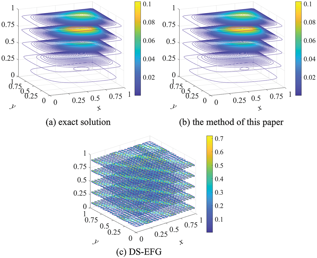
Figure 1: The contour distribution of the exact and numerical solutions at z=0.1,0.3,0.5,0.7,0.9 for Example 1

When the small coefficients are respectively κ=10−6,10−9,10−12,10−15,10−18, the corresponding relative errors for 41×41×21 and 65×65×26 regular nodes distributions are shown in Table 1. The results show that for almost singular diffusion coefficients, our method of this paper still has a very stable solution.

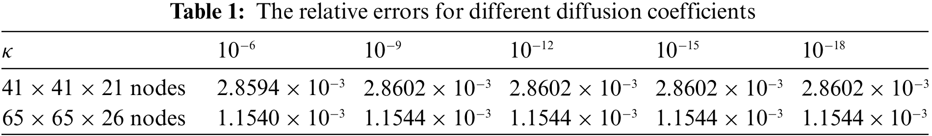
When the nodes distribution is 41×41×21, the relative errors for different values of dmax=1.1,1.2,⋯,3 are given in Fig. 2. This figure shows that the DS-VMIEFG method of this paper has higher numerical accuracy when dmax is around 1.2.

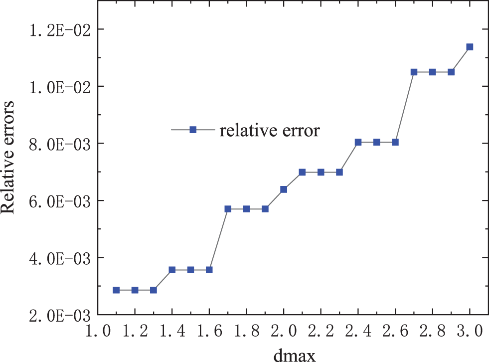
Figure 2: The relative errors for different values of dmax=1.1,1.2,⋯,3 with the nodes distribution 41×41×21

To study the convergence, when there are 21 splitting points in the z direction and 17×17, 33×33,65×65,129×129 nodes on the 2D splitting surface, the relative errors are shown in Fig. 3. It can be seen that as the number of nodes increases, the numerical solution gradually converges to the exact solution.

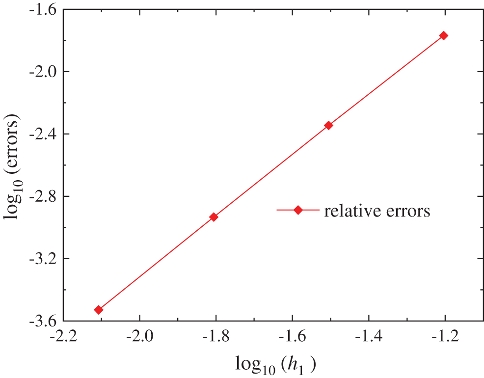
Figure 3: The relative errors for different regular nodes distribution of 17×17, 33×33, 65×65, 129×129 nodes on the 2D splitting surface with dmax=1.2 and h3=0.05

Example 2. The second considered convection-diffusion problem has the following exact solution as [62]

u(x,y,z)=sin⁡(πx)sin⁡(πz)sin⁡(πy),(x,y,z)∈Ω=[0,1]×[0,1]×[0,1].(51)

The parameters are a1=cos⁡α⋅cos⁡β,a2=cos⁡α⋅sin⁡β,a3=sin⁡α, where α=35o,β=45o. The source term f and the boundary conditions are obtained from the analytical solution of Eq. (51).

When κ=10−9 and applying the regular 41×41×21 nodes distribution, we presented the contour distribution of the solution at z=0.1,0.3,0.5,0.7,0.9 in Fig. 4 with dmax=1.2. And results of the method of this paper and the DS-EFG method are respectively shown in Figs. 4b and 4c. The numerical results of our method agree well with the exact. However, the contours solved by the DS-EFG method have obvious oscillations.

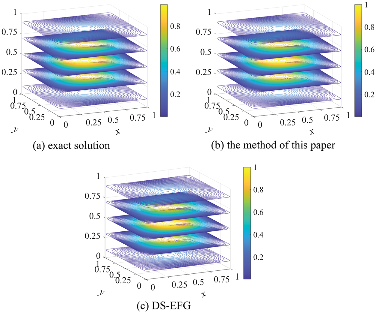
Figure 4: The contour distributions of the exact and numerical solutions at z=0.1,0.3,0.5,0.7,0.9 for Example 2

When κ=10−6,10−9,10−12,10−15,10−18, the corresponding relative errors for 41×41×11 and 65×65×21 regular nodes distributions are shown in Table 2. It can be seen from the results that the DS-VMIEFG method in this paper can still obtain higher precision solutions for the convection-diffusion problems with high singular diffusion coefficients.

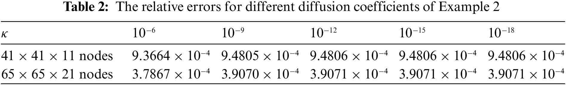
When using the regular 41×41×11 nodes distribution, we plot the relative errors of different dmax=1.1,1.2,⋯,3 in Fig. 5. It can be seen that when the value of dmax is around 1.2, the method in this paper can obtain higher calculation accuracy.

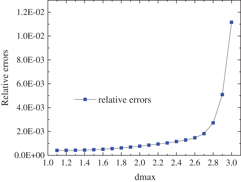
Figure 5: The relative errors for different values of dmax=1.1,1.2,⋯,3 with the nodes distribution 65×65×11 for Example 2

When 21 splitting points are fixed in the z direction, for different node distributions of 17×17, 33×33,65×65,129×129 nodes on the 2D split plane, the relative errors are shown in Fig. 6. The results show that the solution of the numerical method in this paper is convergent.

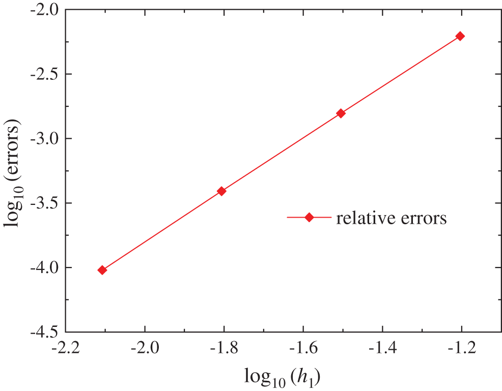
Figure 6: The relative errors for different regular nodes distribution of 17×17, 33×33, 65×65, 129×129 nodes on the 2D splitting surface with dmax=1.2 and h3=0.05 for Example 2

5  Conclusions

By introducing the DS method into the VMIEFG method, a DS-VMIEFG method for three-dimensional singular perturbed convection-diffusion problems is presented in this paper. In the DS-VMIEFG method, the 3D problem is decomposed into a series of 2D problems, and then the weak form of the Galerkin integral is only established on the 2D splitting surfaces by the VMIEFG method. The DS-VMIEFG method can avoid the construction of integral weak form on the 3D domain. The IIMLS method is used to obtain the shape functions in the weak form and to combine 2D discrete equations into a global system of discrete equations for the 3D SPCD problems. The numerical example verifies the effectiveness of the DS-VMIEFG method in the case of very small singularly perturbed diffusion coefficients, and the numerical solution can avoid non-physical numerical oscillations.

Funding Statement: This work is supported by the Natural Science Foundation of Zhejiang Province, China (Grant Nos. LY20A010021, LY19A010002, LY20G030025), and the Natural Science Foundation of Ningbo City, China (Grant Nos. 2021J147, 2021J235).

Conflicts of Interest: The authors declare that they have no conflicts of interest to report regarding the present study.

References

 1.  Gu, Y., Fan, C., Xu, R. (2019). Localized method of fundamental solutions for large-scale modeling of two-dimensional elasticity problems. Applied Mathematics Letters, 93(7), 8–14. DOI 10.1016/j.aml.2019.01.035. [Google Scholar] [CrossRef]

 2.  Zhang, T., Li, X. (2020). Variational multiscale interpolating element-free Galerkin method for the nonlinear Darcy-Forchheimer model. Computers & Mathematics with Applications, 79(2), 363–377. DOI 10.1016/j.camwa.2019.07.003. [Google Scholar] [CrossRef]

 3.  Gu, Y., Fan, C., Qu, W., Wang, F. (2019). Localized method of fundamental solutions for large-scale modelling of three-dimensional anisotropic heat conduction problems-theory and matlab code. Computers & Structures, 220, 144–155. DOI 10.1016/j.compstruc.2019.04.010. [Google Scholar] [CrossRef]

 4.  Wang, J., Sun, F. (2019). A hybrid variational multiscale element-free Galerkin method for convection-diffusion problems. International Journal of Applied Mechanics, 11(7), 1950063. DOI 10.1142/S1758825119500637. [Google Scholar] [CrossRef]

 5.  Gu, Y., Sun, H. (2020). A meshless method for solving three-dimensional time fractional diffusion equation with variable-order derivatives. Applied Mathematical Modelling, 78, 539–549. DOI 10.1016/j.apm.2019.09.055. [Google Scholar] [CrossRef]

 6.  Abbaszadeh, M., Khodadadian, A., Parvizi, M., Dehghan, M., Heitzinger, C. (2019). A direct meshless local collocation method for solving stochastic cahn-hilliard–cook and stochastic swift-hohenberg equations. Engineering Analysis with Boundary Elements, 98(2), 253–264. DOI 10.1016/j.enganabound.2018.10.021. [Google Scholar] [CrossRef]

 7.  Selim, B. A., Liu, Z. (2021). Impact analysis of functionally-graded graphene nanoplatelets-reinforced composite plates laying on winkler-pasternak elastic foundations applying a meshless approach. Engineering Structures, 241(5), 112453. DOI 10.1016/j.engstruct.2021.112453. [Google Scholar] [CrossRef]

 8.  Almasi, F., Shadloo, M. S., Hadjadj, A., Ozbulut, M., Tofighi, N. et al. (2021). Numerical simulations of multi-phase electro-hydrodynamics flows using a simple incompressible smoothed particle hydrodynamics method. Computers & Mathematics with Applications, 81(10), 772–785. DOI 10.1016/j.camwa.2019.10.029. [Google Scholar] [CrossRef]

 9.  Peng, P., Fu, Y., Cheng, Y. (2021). A hybrid reproducing kernel particle method for three-dimensional advection-diffusion problems. International Journal of Applied Mechanics, 13(7), 2150085. DOI 10.1142/S175882512150085X. [Google Scholar] [CrossRef]

10. Nguyen, V. P., Rabczuk, T., Bordas, S., Duflot, M. (2008). Meshless methods: A review and computer implementation aspects. Mathematics and Computers in Simulation, 79(3), 763–813. DOI 10.1016/j.matcom.2008.01.003. [Google Scholar] [CrossRef]

11. Chen, J. S., Hillman, M., Chi, S. W. (2017). Meshfree methods: Progress made after 20 years. Journal of Engineering Mechanics, 143(4), 4017001. DOI 10.1061/(ASCE)EM.1943-7889.0001176. [Google Scholar] [CrossRef]

12. Liu, M., Zhang, Z. (2019). Smoothed particle hydrodynamics (SPH) for modeling fluid-structure interactions. Science China Physics, Mechanics & Astronomy, 62(8), 1–38. DOI 10.1007/s11433-018-9357-0. [Google Scholar] [CrossRef]

13. Solanki, M. K., Mishra, S. K., Singh, J. (2016). Meshfree approach for linear and nonlinear analysis of sandwich plates: A critical review of twenty plate theories. Engineering Analysis with Boundary Elements, 69(8), 93–103. DOI 10.1016/j.enganabound.2016.05.002. [Google Scholar] [CrossRef]

14. Li, Y., Liu, G. R. (2019). An element-free smoothed radial point interpolation method (EFS-RPIM) for 2D and 3D solid mechanics problems. Computers & Mathematics with Applications, 77(15), 441–465. DOI 10.1016/j.camwa.2018.09.047. [Google Scholar] [CrossRef]

15. Cheng, J. (2021). Mathematical models and data analysis of residential land leasing behavior of district governments of Beijing in China. Mathematics, 9(18), 2314. DOI 10.3390/math9182314. [Google Scholar] [CrossRef]

16. Cheng, J., Xie, Y., Zhang, J. (2022). Industry structure optimization via the complex network of industry space: A case study of Jiangxi Province in China. Journal of Cleaner Production, 338(1), 130602. DOI 10.1016/j.jclepro.2022.130602. [Google Scholar] [CrossRef]

17. Cheng, J., Luo, X. (2022). Analyzing the land leasing behavior of the government of Beijing, China, via the multinomial logit model. Land, 11(3), 376. DOI 10.3390/land11030376. [Google Scholar] [CrossRef]

18. Lancaster, P., Salkauskas, K. (1981). Surfaces generated by moving least squares methods. Mathematics of Computation, 37(155), 141–158. DOI 10.1090/S0025-5718-1981-0616367-1. [Google Scholar] [CrossRef]

19. Chen, S., Duan, Q. (2020). An adaptive second-order element-free Galerkin method for additive manufacturing process. Computational Materials Science, 183(2), 109911. DOI 10.1016/j.commatsci.2020.109911. [Google Scholar] [CrossRef]

20. Ye, T., Li, Y. (2018). A comparative review of smoothed particle hydrodynamics, dissipative particle dynamics and smoothed dissipative particle dynamics. International Journal of Computational Methods, 15(8), 1850083. DOI 10.1142/S0219876218500834. [Google Scholar] [CrossRef]

21. Singh, R., Singh, K. M. (2019). Interpolating meshless local petrov-Galerkin method for steady state heat conduction problem. Engineering Analysis with Boundary Elements, 101, 56–66. DOI 10.1016/j.enganabound.2018.12.012. [Google Scholar] [CrossRef]

22. Garg, S., Pant, M. (2018). Meshfree methods: A comprehensive review of applications. International Journal of Computational Methods, 15(4), 1830001. DOI 10.1142/S0219876218300015. [Google Scholar] [CrossRef]

23. Liew, K. M., Feng, C., Cheng, Y., Kitipornchai, S. (2007). Complex variable moving least-squares method: A meshless approximation technique. International Journal for Numerical Methods in Engineering, 70(1), 46–70. DOI 10.1002/(ISSN)1097-0207. [Google Scholar] [CrossRef]

24. Li, X., Li, S. (2017). Improved complex variable moving least squares approximation for three-dimensional problems using boundary integral equations. Engineering Analysis with Boundary Elements, 84(2), 25–34. DOI 10.1016/j.enganabound.2017.08.003. [Google Scholar] [CrossRef]

25. Wang, J. F., Sun, F., Cheng, Y., Huang, A. X. (2014). Error estimates for the interpolating moving least-squares method. Applied Mathematics and Computation, 245(1), 321–342. DOI 10.1016/j.amc.2014.07.072. [Google Scholar] [CrossRef]

26. Wang, J., Wang, J., Sun, F., Cheng, Y. (2013). An interpolating boundary element-free method with nonsingular weight function for two-dimensional potential problems. International Journal of Computational Methods, 10(6), 1350043. DOI 10.1142/S0219876213500436. [Google Scholar] [CrossRef]

27. Sun, F. X., Wang, J. F., Cheng, Y. M., Huang, A. X. (2015). Error estimates for the interpolating moving least-squares method in n-dimensional space. Applied Numerical Mathematics, 98, 79–105. DOI 10.1016/j.apnum.2015.08.001. [Google Scholar] [CrossRef]

28. Sun, F., Wang, J., Cheng, Y. (2016). An improved interpolating element-free Galerkin method for elastoplasticity via nonsingular weight functions. International Journal of Applied Mechanics, 8(8), 1650096. DOI 10.1142/S1758825116500964. [Google Scholar] [CrossRef]

29. Belytschko, T., Lu, Y. Y., Gu, L. (1994). Element-free Galerkin methods. International Journal for Numerical Methods in Engineering, 37(2), 229–256. DOI 10.1002/(ISSN)1097-0207. [Google Scholar] [CrossRef]

30. Abbaszadeh, M., Dehghan, M. (2019). The interpolating element-free Galerkin method for solving Korteweg-de Vries-Rosenau-regularized long-wave equation with error analysis. Nonlinear Dynamics, 96(2), 1345–1365. DOI 10.1007/s11071-019-04858-1. [Google Scholar] [CrossRef]

31. Cheng, Y. M., Bai, F. N., Peng, M. J. (2014). A novel interpolating element-free Galerkin (IEFG) method for two-dimensional elastoplasticity. Applied Mathematical Modelling, 38(21–22), 5187–5197. DOI 10.1016/j.apm.2014.04.008. [Google Scholar] [CrossRef]

32. Wang, J., Sun, F. (2019). An interpolating meshless method for the numerical simulation of the time-fractional diffusion equations with error estimates. Engineering Computations, 37(2), 730–752. DOI 10.1108/EC-03-2019-0117. [Google Scholar] [CrossRef]

33. Wang, J., Sun, F., Xu, Y. (2020). Research on error estimations of the interpolating boundary element free-method for two-dimensional potential problems. Mathematical Problems in Engineering, 2020, 6378710–6378745. DOI 10.1155/2020/6378745. [Google Scholar] [CrossRef]

34. Wang, J., Sun, F., Cheng, Y. (2012). An improved interpolating element-free Galerkin method with a nonsingular weight function for two-dimensional potential problems. Chinese Physics B, 21(9), 90204. DOI 10.1088/1674-1056/21/9/090204. [Google Scholar] [CrossRef]

35. Liu, D., Cheng, Y. M. (2019). The interpolating element-free Galerkin (IEFG) method for three-dimensional potential problems. Engineering Analysis with Boundary Elements, 108(1–4), 115–123. DOI 10.1016/j.enganabound.2019.08.021. [Google Scholar] [CrossRef]

36. Chen, S., Wang, J. (2017). Coupled interpolating element-free Galerkin scaled boundary method and finite element method for crack problems. Scientia Sinica Physica, Mechanica & Astronomica, 48(2), 24601. DOI 10.1360/SSPMA2017-00283. [Google Scholar] [CrossRef]

37. Chen, S., Wang, W., Zhao, X. (2019). An interpolating element-free Galerkin scaled boundary method applied to structural dynamic analysis. Applied Mathematical Modelling, 75, 494–505. DOI 10.1016/j.apm.2019.05.041. [Google Scholar] [CrossRef]

38. Abbaszadeh, M., Dehghan, M., Khodadadian, A., Heitzinger, C. (2020). Analysis and application of the interpolating element free Galerkin (IEFG) method to simulate the prevention of groundwater contamination with application in fluid flow. Journal of Computational and Applied Mathematics, 368, 112453. DOI 10.1016/j.cam.2019.112453. [Google Scholar] [CrossRef]

39. Wu, Q., Liu, F. B., Cheng, Y. M. (2020). The interpolating element-free Galerkin method for three-dimensional elastoplasticity problems. Engineering Analysis with Boundary Elements, 115(1), 156–167. DOI 10.1016/j.enganabound.2020.03.009. [Google Scholar] [CrossRef]

40. Zhang, X., Hu, Z., Wang, M. (2021). An adaptive interpolation element free Galerkin method based on a posteriori error estimation of FEM for poisson equation. Engineering Analysis with Boundary Elements, 130(1), 186–195. DOI 10.1016/j.enganabound.2021.05.020. [Google Scholar] [CrossRef]

41. Wu, Q., Peng, P. P, Cheng, Y. M. (2021). The interpolating element-free Galerkin method for elastic large deformation problems. Science China Technological Sciences, 64(2), 364–374. DOI 10.1007/s11431-019-1583-y. [Google Scholar] [CrossRef]

42. Abbaszadeh, M., Dehghan, M. (2020). Investigation of the oldroyd model as a generalized incompressible Navier-Stokes equation via the interpolating stabilized element free Galerkin technique. Applied Numerical Mathematics, 150, 274–294. DOI 10.1016/j.apnum.2019.08.025. [Google Scholar] [CrossRef]

43. Wang, J., Sun, F., Cheng, R. (2021). A dimension splitting-interpolating moving least squares (DS-IMLS) method with nonsingular weight functions. Mathematics, 9(19), 2424. DOI 10.3390/math9192424. [Google Scholar] [CrossRef]

44. Meng, Z., Cheng, H., Ma, L., Cheng, Y. (2019). The dimension splitting element-free Galerkin method for 3D transient heat conduction problems. Science China Physics, Mechanics & Astronomy, 62(4), 1–12. DOI 10.1007/s11433-018-9299-8. [Google Scholar] [CrossRef]

45. Wu, Q., Peng, M., Cheng, Y. (2021). The interpolating dimension splitting element-free Galerkin method for 3D potential problems. Engineering with Computers. DOI 10.1007/s00366-021-01408-5. [Google Scholar] [CrossRef]

46. Ma, L., Meng, Z., Chai, J., Cheng, Y. (2020). Analyzing 3D advection-diffusion problems by using the dimension splitting element-free Galerkin method. Engineering Analysis with Boundary Elements, 111(3), 167–177. DOI 10.1016/j.enganabound.2019.11.005. [Google Scholar] [CrossRef]

47. Cheng, H., Peng, M. J., Cheng, Y. M. (2018). The dimension splitting and improved complex variable element-free Galerkin method for 3-Dimensional transient heat conduction problems. International Journal for Numerical Methods in Engineering, 114(3), 321–345. DOI 10.1002/nme.5745. [Google Scholar] [CrossRef]

48. Peng, P. P., Cheng, Y. M. (2020). Analyzing three-dimensional transient heat conduction problems with the dimension splitting reproducing kernel particle method. Engineering Analysis with Boundary Elements, 121(2), 180–191. DOI 10.1016/j.enganabound.2020.09.011. [Google Scholar] [CrossRef]

49. Wu, Q., Peng, M. J., Fu, Y. D., Cheng, Y. M. (2021). The dimension splitting interpolating element-free Galerkin method for solving three-dimensional transient heat conduction problems. Engineering Analysis with Boundary Elements, 128(1–4), 326–341. DOI 10.1016/j.enganabound.2021.04.016. [Google Scholar] [CrossRef]

50. Cheng, H., Peng, M., Cheng, Y., Meng, Z. (2020). The hybrid complex variable element-free Galerkin method for 3D elasticity problems. Engineering Structures, 219(2), 110835. DOI 10.1016/j.engstruct.2020.110835. [Google Scholar] [CrossRef]

51. Meng, Z., Chi, X. (2022). An improved interpolating dimension splitting element-free Galerkin method for 3D wave equations. Engineering Analysis with Boundary Elements, 134(1–3), 96–106. DOI 10.1016/j.enganabound.2021.09.027. [Google Scholar] [CrossRef]

52. Peng, P., Cheng, Y. (2021). Analyzing three-dimensional wave propagation with the hybrid reproducing kernel particle method based on the dimension splitting method. Engineering with Computers, 38, 1131–1147. DOI 10.1007/s00366-020-01256-9. [Google Scholar] [CrossRef]

53. Zhang, L., Ouyang, J., Wang, X., Zhang, X. (2010). Variational multiscale element-free Galerkin method for 2D burgers’ equation. Journal of Computational Physics, 229(19), 7147–7161. DOI 10.1016/j.jcp.2010.06.004. [Google Scholar] [CrossRef]

54. Dehghan, M., Abbaszadeh, M. (2016). Proper orthogonal decomposition variational multiscale element free Galerkin (POD-VMEFG) meshless method for solving incompressible Navier-Stokes equation. Computer Methods in Applied Mechanics and Engineering, 311(10), 856–888. DOI 10.1016/j.cma.2016.09.008. [Google Scholar] [CrossRef]

55. Cao, X., Zhang, X., Shi, X. (2022). An adaptive variational multiscale element free Galerkin method based on the residual-based a posteriori error estimators for convection-diffusion-reaction problems. Engineering Analysis with Boundary Elements, 136(1–3), 238–251. DOI 10.1016/j.enganabound.2022.01.001. [Google Scholar] [CrossRef]

56. Sun, F., Wang, J., Kong, X., Cheng, R. (2021). A dimension splitting generalized interpolating element-free Galerkin method for the singularly perturbed steady convection-diffusion–reaction problems. Mathematics, 9(19), 2524. DOI 10.3390/math9192524. [Google Scholar] [CrossRef]

57. Wang, J., Sun, F. (2020). A hybrid generalized interpolated element-free Galerkin method for stokes problems. Engineering Analysis with Boundary Elements, 111(3), 88–100. DOI 10.1016/j.enganabound.2019.11.002. [Google Scholar] [CrossRef]

58. Sun, H., Xu, Y., Lin, J., Zhang, Y. (2021). A space-time backward substitution method for three-dimensional advection-diffusion equations. Computers & Mathematics with Applications, 97(8), 77–85. DOI 10.1016/j.camwa.2021.05.025. [Google Scholar] [CrossRef]

59. Li, J., Zhao, J., Qian, L., Feng, X. (2018). Two-level meshless local Petrov Galerkin method for multi-dimensional nonlinear convection-diffusion equation based on radial basis function. Numerical Heat Transfer, Part B: Fundamentals, 74(4), 685–698. DOI 10.1080/10407790.2018.1538288. [Google Scholar] [CrossRef]

60. Chandhini, G., Sanyasiraju, Y. (2007). Local RBF-FD solutions for steady convection-diffusion problems. International Journal for Numerical Methods in Engineering, 72(3), 352–378. DOI 10.1002/(ISSN)1097-0207. [Google Scholar] [CrossRef]

61. Bullo, T. A., Duressa, G. F., Degla, G. A. (2021). Robust finite difference method for singularly perturbed two-parameter parabolic convection-diffusion problems. International Journal of Computational Methods, 18(2), 2050034. DOI 10.1142/S0219876220500346. [Google Scholar] [CrossRef]

62. Oruç, Ö. (2020). A meshless multiple-scale polynomial method for numerical solution of 3D convection-diffusion problems with variable coefficients. Engineering with Computers, 36(4), 1215–1228. DOI 10.1007/s00366-019-00758-5. [Google Scholar] [CrossRef]

63. Zhang, T., Li, X. (2017). A variational multiscale interpolating element-free Galerkin method for convection-diffusion and stokes problems. Engineering Analysis with Boundary Elements, 82, 185–193. DOI 10.1016/j.enganabound.2017.06.013. [Google Scholar] [CrossRef]

64. Masud, A., Khurram, R. A. (2004). A multiscale/stabilized finite element method for the advection-diffusion equation. Computer Methods in Applied Mechanics and Engineering, 193(21–22), 1997–2018. DOI 10.1016/j.cma.2003.12.047. [Google Scholar] [CrossRef]