
 Submit a Paper
 Propose a Special lssue
 Open Access
ARTICLE
Skeleton-Based Volumetric Parameterizations for Lattice Structures
1 School of Mechanical Engineering, University of Shanghai for Science and Technology, Shanghai, 200093, China
2 School of Optical-Electrical and Computer Engineering, University of Shanghai for Science and Technology, Shanghai, 200093, China
3 Key Laboratory of Education Ministry for Modern Design & Rotor-Bearing System, Xi’an Jiaotong University, Xi’an, 710049, China
* Corresponding Author: Long Chen. Email:
(This article belongs to the Special Issue: Integration of Geometric Modeling and Numerical Simulation)
Computer Modeling in Engineering & Sciences 2023, 135(1), 687-709. https://doi.org/10.32604/cmes.2022.021986
Received 16 February 2022; Accepted 23 May 2022; Issue published 29 September 2022
 View Full Text
 Download PDF
Abstract
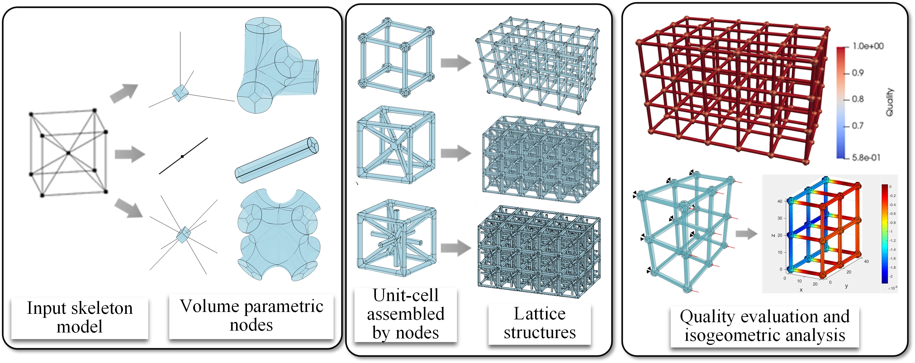
Lattice structures with excellent physical properties have attracted great research interest. In this paper, a novel volume parametric modeling method based on the skeleton model is proposed for the construction of three-dimensional lattice structures. The skeleton model is divided into three types of nodes. And the corresponding algorithms are utilized to construct diverse types of volume parametric nodes. The unit-cell is assembled with distinct nodes according to the geometric features. The final lattice structure is created by the periodic arrangement of unit-cells. Several different types of volume parametric lattice structures are constructed to prove the stability and applicability of the proposed method. The quality is assessed in terms of the value of the Jacobian matrix. Moreover, the volume parametric lattice structures are tested with the isogeometric analysis to verify the feasibility of integration of modeling and simulation.Graphic Abstract
Keywords
In recent years, the extensive application of additive manufacturing (AM) has rendered possibilities for fabricating complex components, such as lattice structures [1]. The lattice structures exhibit low density, enhanced energy absorption, and excellent mechanical properties [2–4]. It is widely used in the aerospace, petrochemical, and manufacturing industries as well as other fields [5]. Most researches on lattice structures focus on the boundary representation (B-rep) models, which require to be transformed into a triangular or quadrangular mesh before simulation [6,7]. However, generating the mesh takes 80% of the time in the entire design and analysis process [8], resulting in a serious reduction in productivity. Therefore, a unified geometric description of modeling and simulation has great advantages. The novel method of isogeometric analysis (IGA) [9] utilizes the same spline basis functions for geometric modeling and physical simulation making it possible to achieve the goal. Many studies have shown that the IGA has higher accuracy and robustness than the finite element analysis (FEA) [10]. It is of great significance to construct a model suitable for IGA.
In this paper, a volume parametric modeling method of three-dimensional (3D) lattice structures is proposed based on the skeleton. The models constructed by our method are suitable for IGA without any transformation. In the entire modeling process, the construction of the volume parametric nodes is the key step. The unit-cell is assembled with different nodes by permutation and combination. And the lattice structure is created via the periodic arrangement of unit-cells. In addition, the toric surface is used as the transition surface to make the shape of the node smooth, which is beneficial to reduce stress concentration in the analysis. The main contributions are as follows:
1. A volume parametric modeling method of complex nodes is achieved.
2. Different types of volume parametric unit-cells and lattice structures are created.
3. The framework of integration of modeling and simulation is completed.
The remainder of the paper is organized as follows: In Section 2, some backgrounds and related works are introduced. The basic theory and algorithms are explained in Section 3. The modeling method of nodes is described in Section 4. The construction processes of unit-cells and lattice structures are presented in Section 5. Several models are provided to verify the effectiveness and the feasibility of the proposed method in Section 6. Finally, the conclusions are summarized in Section 7.
The lattice structures with excellent properties have been widely applied in many industries. Researchers have proposed numerous modeling methods to construct lattice structures. Fan et al. [11] designed a honeycomb lattice structure and a sandwich structure with better mechanical properties than the solid structure, but the model is only two-dimensional. Masalha et al. [12] studied several algorithms to construct heterogeneous or trivariate fillets that support smooth filleting operation. The results verify the feasibility of the algorithms. Li et al. [13] proposed an improved algorithm based on the quartet structure generation set method. The algorithm reconstructed the 3D random porous structure. Leblanc et al. [14] introduced a modeling method based on the block to construct the complex model. The quality of the model heavily relies on the subdivision. Tang et al. [15] presented a novel design method for the periodic lattice structure. The frame generation algorithm is used to generate lattice wireframes based on the kernel. Tang et al. [16] studied an innovative hybrid geometric modeling method of lattice structures with three-stage, which involves generating lattice frames, constructing geometric functions, and voxelization. Liu et al. [17] proposed a memory-efficient modeling method and an adaptive slice algorithm of lattice structure to assist manufacturing. Lattice has an excellent performance in macrostructure as well as in microstructure simulation, such as multiscale crystal defect dynamics [18–22]. It offers a possible solution to study crystalline plasticity on the nanoscale and mesoscale.
Manufacturing lattice structures is not easy via traditional processing technology due to the complex structure. The development of AM solves this problem. Dong et al. [23] summarized the existing modeling approaches and the characteristics of different AM in manufacturing cellular materials. Medeiros et al. [24] proposed an automatic adaptive voids algorithm with AM constraints to fabricate cellular structures with minimal material and maximum strength. Tang et al. [25] presented a method to connect the design and manufacturing process to improve the stiffness of heterogeneous lattice structures with manufacturing constraints. Garner et al. [26] utilized the optimization of individual cells and neighboring pairs to find the best connectivity and smoothness of the physical properties among the microstructures. Conde-Rodríguez et al. [27] proposed a modeling framework of heterogeneous structures based on Bezier patches. The method is appropriate to fabricate structures with different materials, but only single-level details and Bezier were permitted.
Compared with the B-rep models mentioned above, the volume parametric models utilize high-order non-uniform rational B-spline (NURBS) to express the physical domains precisely [28] and are suitable for IGA without any transformation. Meanwhile, the shape of the model remains unchanged after the refinement. On account of those characteristics, the volume parametric model has attracted a lot of attention. To make use of IGA more convenient, an interactive parametric design-analysis platform is designed [29]. In the meantime, many parametric design methods have been proposed [30–33], which greatly extend the geometric modeling method. Moreover, Xiao et al. [34] utilized the surface interrogation technique for IGA and applied it to large-scale lattice-skin structures of several thousand intersections. Li et al. [35] investigated the behavior of functionally graded porous plates reinforced by graphene platelets, and incorporated within the IGA framework. Furthermore, different spline basis functions such as T-spline and PHT are utilized to construct the volume parametric model [36,37]. These methods simplify the parameterization process and extend the application of IGA.
In this paper, a volume parametric modeling method of lattice structures based on the skeleton model is proposed. The method solves the problem of hexahedron segmentation of the complex nodes. And the modeling process is simplified by utilizing volume parametric nodes to assemble lattice structures. In addition, the toric surface is used as the transition surface to make the shape of the node smooth. Most importantly, the model constructed by the proposed method is suitable for isogeometric analysis. The proposed method realizes the integration of modeling and simulation.
3 Basic Theories and Overview of the Algorithm
3.1 Representation of the Volumetric Parameterization Model
The physical domain is defined based on the NURBS [38] and represented by
The volume parametric model and NURBS basis function are described in Eqs. (2) and (3).
where
The skeleton is an abstract description of the geometric model. It is widely used in segmentation, reconstruction, and geometric design. Many extraction algorithms are used to construct the skeleton model [39–42]. The interactive design is the most commonly used method of skeleton construction [43]. For periodic lattice structures, the unit-cell can be utilized to represent the topological information. In this paper, we build the skeleton model of unit-cells according to the different types of lattice structures and given by interconnected NURBS curves. The relationship of the skeleton is expressed by Eq. (4). Two typical lattice structure skeleton models are shown in Fig. 1.

Figure 1: Typical skeleton models of the lattice structure. (a) Honeycomb lattice structure; (b) 3D cubic lattice structure
The unit-cell is the basic element to generate a uniform lattice structure. Several representative unit-cells presented by the skeleton models are shown in Fig. 2.

Figure 2: Typical unit-cell models obtained using the skeleton model
In this paper, we defined three types of nodes according to the number of branches. One branch indicates the end nodes

Figure 3: Node models obtained with the skeleton curves. (a)
The connection part between nodes is composed of solid cylinders. It is divided into five primitive volumes to satisfy the parameterization requirement, as shown in Fig. 4a. The cross-section of the cylinder is composed of B-spline surfaces

Figure 4: The five primitive volumes. (a) Cross-section; (b) volume parametric modeling
The input parameters to the algorithm include the skeleton model

Figure 5: Algorithmic flow of the volume parametric lattice structure modeling
4.1 Inner Hexahedral Group Construction of the Branch Node
Based on the research of the previous work [31], this study implements a “skeleton-aware” hexahedra group generation method. Firstly, an initial hexahedral box
The posture redirection operation ensures the branch curves penetrate from different surfaces of
This is a nonlinear optimization problem. The length of the orthogonal basis

Figure 6: Inner hexahedron group generation. (a) Posture redirection operation; (b) volume subdivision operation; (c) branch generation
After the posture redirection operation, there may still exist more one branch curves intersect with the same surface
Each surface of
4.2 Outer Hexahedral Group Construction of the Branch Node
The outer hexahedrons of the node are constructed based on the inner hexahedron group modeling after the above steps. Firstly, construct the transition surfaces of the node. Then, the inner hexahedron group converts into multiple B-spline surfaces. Finally, the volume interpolation is used to generate the outer hexahedron group.
A toric surface is adopted here to create a closed surface of the node mostly because of the advantages of good smoothness [44,45]. The construction algorithm is based on the multilateral Coons interpolation algorithm. Taking
Here,
It is necessary to segment the outer surface to construct a closed transition surface. The intersection points of the sampling vector

Figure 7: Toric surface
Supposing there are
When the boundary surface in

Figure 8: Calculate sampling vectors and corner vectors. (a) Sampling vectors of the boundary surface; (b) calculate corner sampling vector
The vector of each corner
When the corner point
The sampling vector on the edge
The Newton iteration method is used to find the intersection points on the transition surface. The sampling points and the Coons interpolation algorithm are used to fit the B-spline curves

Figure 9: Outer hexahedron group modeling. (a) Boundary surface and transition surface mapping; (b) outer hexahedron group
According to the mapping between
The local patches of the outer hexahedron group and the final volume parametric node are shown in Fig. 9b.
4.3 Modeling of Joint Nodes and End Nodes
After completing the modeling of the branch node, the cross-section is obtained, as shown in Fig. 4a. Each cross-section is expressed by Eq. (14).
The end node
The stretch volumes are constructed through affine transformations of the section group along the skeleton curve as shown in Fig. 10a.

Figure 10: Node modeling. (a) Extruding; (b) sweeping; (c) lofting
In addition, sweeping is another method to construct nodes. Both
The other control points
Here,
The joint node is constructed with the two section groups
5 Modeling of the Unit Cell and the Lattice Structure
The unit-cell of the lattice structure describes the local characteristics. The geometric parameters that control the specific shape of the unit-cell mainly include the size (i.e., length, width, and height), section radius, and horizontal angles. According to the geometry and topology of the skeleton model, a volume parametric unit-cell is constructed through translation, rotation, and reflection of the nodes. The relationship between the unit-cell
For example, the skeleton of the simple cubic unit-cell shown in Fig. 11c is split into two basic nodes, as shown in Figs. 11a and 11b. The volume parametric models of the two nodes are constructed as illustrated in Figs. 11d and 11e. The final unit-cell model is obtained through translation, rotation, and splicing operations, as shown in Fig. 12f.

Figure 11: Simple cubic unit-cell model generation. (a) Node skeleton; (b) node skeleton; (c) unit-cell skeleton; (d) node model; (e) node model; (f) unit-cell model

Figure 12: Simple cubic lattice structure model generation. (a) Unit-cell model; (b) joint node model; (c) lattice structure model
5.2 Modeling of the Lattice Structure
The unit-cell of the uniform lattice structure is a parallelepiped. Three translation basis vectors intersect at the vertex. The skeleton with three orthogonal translation basis vectors is called the cubic lattice structure. Due to the unique symmetry properties, the cubic lattice structure is the most widely used type. The modeling process mainly includes two steps. Firstly, the unit-cell is constructed as the basic element. Secondly, duplicate the unit-cells in space to form the lattice structure. The center of the unit-cell is used to indicate the location. Finally, unit-cells are arranged along the translation basis vectors to generate the volume parametric lattice structures.
A simple cubic lattice structure that satisfies geometric connectivity is shown in Fig.12. The volume parametric unit-cell is composed of 308 trivariate NURBS volumes as shown in Fig. 12a. We set the translation basis vectors as the coordinate axis directions, and a series of operations involving the translation basis vector directions are executed. The connectivity among unit-cells is guaranteed by the joint node as shown in Fig. 12b. The volume parametric lattice structure with 4096 trivariate NURBS volumes is constructed as shown in Fig. 12c.
We constructed several models of node and lattice structure to prove the effectiveness and applicability of the proposed method. In the meantime, the Jacobian values of the models are calculated and visualized to evaluate the quality. And the IGA is utilized to verify the feasibility of integration of modeling and simulation of our method.
6.1 Examples of Branch Node Models
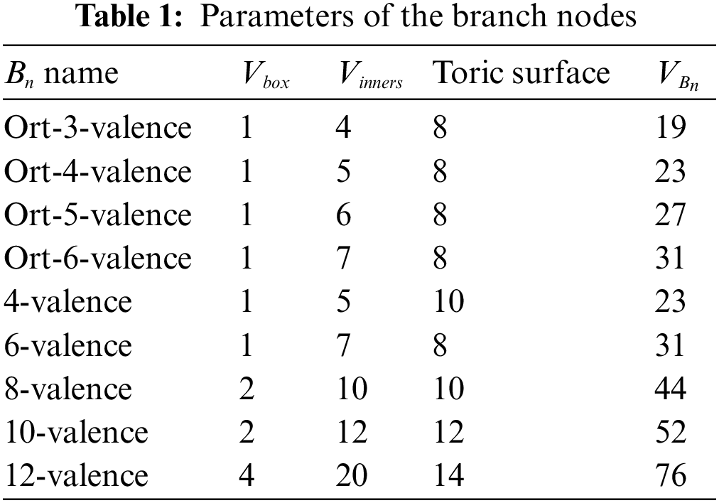
Several nodes are constructed with the modeling method presented in Section 4. The nodes with orthogonal branches are shown in Fig. 13, and the others are shown in Fig. 14. The branch curves with the hexahedron boxes are shown in column (a), the inner hexahedron groups are shown in column (b), the transition surface models constructed with multiple toric surfaces are shown in column (c), and the volume parametric nodes are shown in column (d). The parameters of nodes are listed in Table 1. The first four cases are classified as orthogonal nodes, the length of the branch curves is 2, and the diameter of the cross-section is 2. The last five cases are classified as complex nodes with a length of 3 and the same diameter.

Figure 13: Modeling process of orthogonal branch nodes. (a) Hexahedron box; (b) inner hexahedron groups; (c) transition surfaces; (d) volumetric parameterization nodes

Figure 14: Modeling process of complex branch nodes. (a) Hexahedron box; (b) inner hexahedron groups; (c) transition surfaces; (d) volumetric parameterization nodes
6.2 Examples of Unit-Cell Models
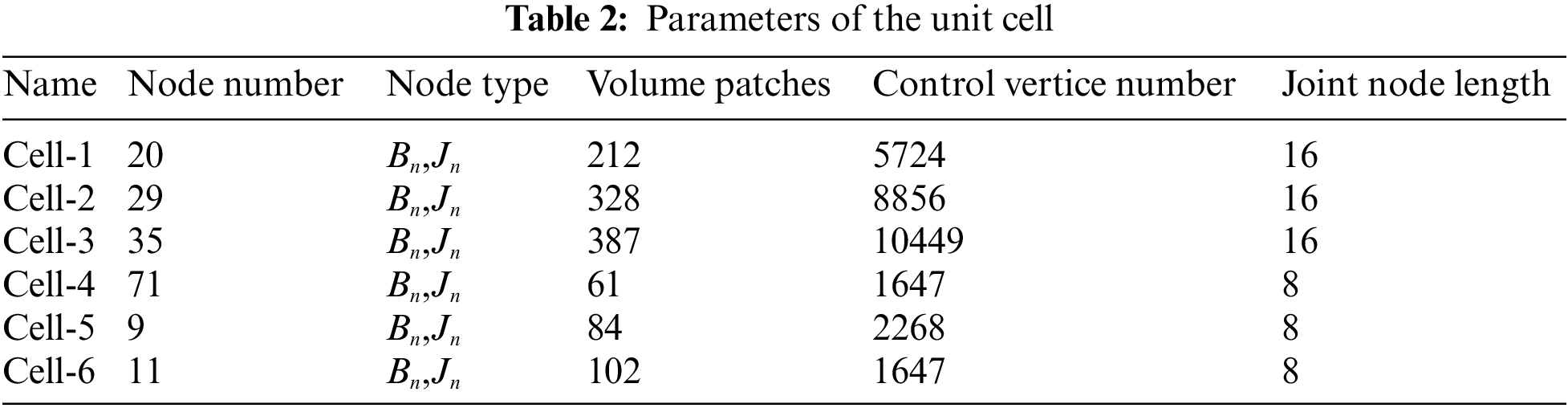
According to Section 5, we construct some typical unit-cell models as shown in Fig.15. The parameters are listed in Table 2. The diameter of the cross-section of joint nodes is 2.

Figure 15: The unit-cell models. (a) Simple cubic unit-cell(Cell-1); (b) body-centered cubic unit-cell(Cell-2); (c) face-body-centered cubic unit-cell(Cell-3); (d) 3D-Kagome unit-cell(Cell-4); (e) 3D-pyramidal unit-cell(Cell-5); (f) body-centered-plus unit-cell(Cell-6)
6.3 Examples of Lattice Structures
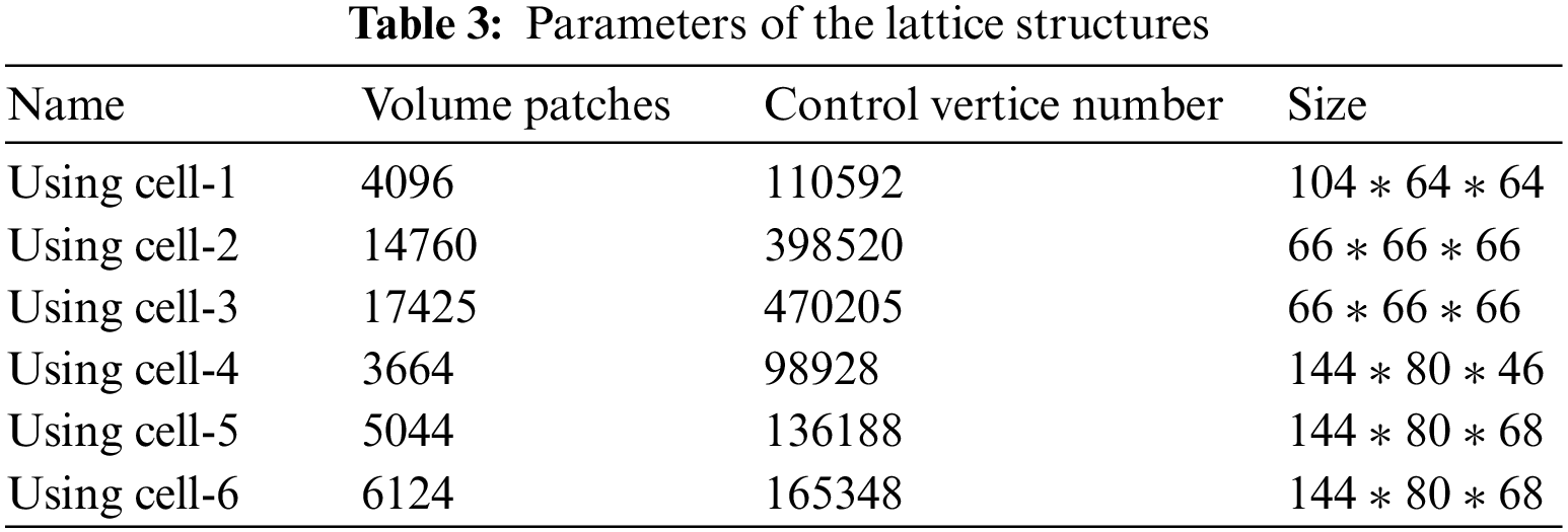
Based on the abovementioned unit-cells, several different types of volume parametric lattice structures are constructed as shown in Fig. 16. Some sandwich-type of lattice structures are also built as shown in Fig. 17. The 3D view of the models is presented in the first column, and the front view is illustrated in the second column. The parameters of the lattice structures are listed in Table 3.

Figure 16: Multiple cubic lattice structure models

Figure 17: Sandwich-type lattice structure models
6.4 Evaluation of the Model Quality
To verify the volume parametric model is suitable for IGA without intersections, overlaps, or large-angle distortions of hexahedrons, the value of the Jacobian matrix is the main index for quality assessment [48–50]. In addition, the Jacobian value should be greater than zero and the distribution should be as evenly as possible within the parameter domain. The calculation of the Jacobian value is provided with the expression Eq. (20).
The Jacobian values of the nodes and the unit cells are shown in Figs. 18–20. The Jacobian values are bigger than zero, and the distribution is relatively symmetrical. The quality evaluation of volume parametric lattice structures is shown in Fig. 21. The Jacobian values demonstrate excellent quality and satisfy the requirement of analysis. Therefore, the quality of the models obtained by the proposed method is verified.

Figure 18: Jacobian values of orthogonal branch nodes

Figure 19: Jacobian values of complex branch nodes

Figure 20: Jacobian values of unit-cell models

Figure 21: Jacobian values of the lattice structure models
There are some singularities in the models constructed by the proposed method, which are reflected in the minimum values of the Jacobian. Singularities damage the quality of the model. How to control the singularity is a major issue of geometric modeling. Researchers have proposed some approaches, such as utilizing sparse distributed directional constraints to determine the appropriate singularities [51], designing different templates to handle the features of new singularities [46], or using a practical framework to adjust singularity graphs by modifying the rotational transition [52]. Some researchers use novel tetrahedral split operations to preprocess singularity-restricted frame fields [53]. These methods achieve the goal of controlling the singularity but bring a huge extra computation at the same time. The model of lattice structure is especially difficult to deal with singularities with complex nodes and massive volume parametric patches. Considering the Jacobian values still meet the requirement of IGA, the singularities are not specifically controlled in the modeling process of this paper.
6.5 Model Verification via IGA
We applicated IGA to the volume parametric models to verify the applicability. As shown in Figs. 22 and 23, the boundary conditions are shown in column (a). We set the material as stainless steel, Young’s modulus is


Figure 22: Results of the IGA and FEA conducted on the unit-cell models

Figure 23: Results of the IGA and FEA conducted on the lattice structure model
The boundary conditions are illustrated in Fig.22a. The load is equal to
With the above examples, we have proved the volume parametric models constructed by our method are suitable for IGA, and the feasibility of integration of modeling and simulation is verified too.
In this paper, a volume parametric modeling method of 3D lattice structures based on the skeleton model is proposed. The unit-cell is combined with different volume parametric nodes. And the volume parametric lattice structure is assembled with the periodic arrangements of the unit-cells. The effectiveness and stability of the proposed method are proved with numerous examples. The quality of the volume parametric models is evaluated by Jacobian values. And finally, the feasibility of integration of modeling and simulation is proved with isogeometric analysis.
However, the quality of complex nodes is still not perfect enough, and how to control the singularity is also an important issue. In addition, the manufacturing of volume parametric lattice structures is worth to be studied in the future, and applying these models to crystal dynamics is also significant.
Funding Statement: This research is supported by the National Nature Science Foundation of China under Grant No. 52075340.
Conflicts of Interest: The authors declare that they have no conflicts of interest to report regarding the present study.
References
1. Chu, C., Graf, G., Rosen, D. W. (2008). Design for additive manufacturing of cellular structures. Computer-Aided Design and Applications, 5(5), 686–696. DOI 10.3722/cadaps.2008.686-696. [Google Scholar] [CrossRef]
2. Schmelzle, J., Kline, E. V., Dickman, C. J., Reutzel, E. W., Jones, G. et al. (2015). (Re) Designing for part consolidation: Understanding the challenges of metal additive manufacturing. Journal of Mechanical Design, 137(11), 111404. DOI 10.1115/1.4031156. [Google Scholar] [CrossRef]
3. Hutchinson, J. W., Xue, Z. (2005). Metal sandwich plates optimized for pressure impulses. International Journal of Mechanical Sciences, 47(4–5), 545–569. DOI 10.1016/j.ijmecsci.2004.10.012. [Google Scholar] [CrossRef]
4. Liu, T., Deng, Z. C., Lu, T. J. (2007). Bi-functional optimization of actively cooled, pressurized hollow sandwich cylinders with prismatic cores. Journal of the Mechanics and Physics of Solids, 55(12), 2565–2602. DOI 10.1016/j.jmps.2007.04.007. [Google Scholar] [CrossRef]
5. Vasiliev, V. V., Razin, A. F. (2006). Anisogrid composite lattice structures for spacecraft and aircraft applications. Composite Structures, 76(1–2), 182–189. DOI 10.1016/j.compstruct.2006.06.025. [Google Scholar] [CrossRef]
6. Hughes, T. J. (2012). The finite element method: Linear static and dynamic finite element analysis. Chelmsford: Courier Corporation. [Google Scholar]
7. Lei, H., Li, C., Meng, J., Zhou, H., Liu, Y. et al. (2019). Evaluation of compressive properties of SLM-fabricated multi-layer lattice structures by experimental test and μ-CT-based finite element analysis. Materials & Design, 169(6058), 107685. DOI 10.1016/j.matdes.2019.107685. [Google Scholar] [CrossRef]
8. Cottrell, J. A., Hughes, T. J., Bazilevs, Y. (2009). Isogeometric analysis: Toward integration of CAD and FEA. Hoboken: John Wiley & Sons. [Google Scholar]
9. Hughes, T. J., Cottrell, J. A., Bazilevs, Y. (2005). Isogeometric analysis: CAD, finite elements, NURBS, exact geometry and mesh refinement. Computer Methods in Applied Mechanics and Engineering, 194(39–41), 4135–4195. DOI 10.1016/j.cma.2004.10.008. [Google Scholar] [CrossRef]
10. Massarwi, F., Elber, G. (2016). A B-spline based framework for volumetric object modeling. Computer-Aided Design, 78(5526), 36–47. DOI 10.1016/j.cad.2016.05.003. [Google Scholar] [CrossRef]
11. Fan, H. L., Jin, F. N., Fang, D. N. (2008). Mechanical properties of hierarchical cellular materials. Part I: Analysis. Composites Science and Technology, 68(15–16), 3380–3387. DOI 10.1016/j.compscitech.2008.09.022. [Google Scholar] [CrossRef]
12. Masalha, R., Cirillo, E., Elber, G. (2021). Heterogeneous parametric trivariate fillets. Computer Aided Geometric Design, 86, 101970. DOI 10.1016/j.cagd.2021.101970. [Google Scholar] [CrossRef]
13. Li, J., Zheng, W., Su, Y., Hong, F. (2022). Pore scale study on capillary pumping process in three-dimensional heterogeneous porous wicks using Lattice Boltzmann method. International Journal of Thermal Sciences, 171, 107236. DOI 10.1016/j.ijthermalsci.2021.107236. [Google Scholar] [CrossRef]
14. Leblanc, L., Houle, J., Poulin, P. (2011). Modeling with blocks. The Visual Computer, 27(6), 555–563. DOI 10.1007/s00371-011-0589-4. [Google Scholar] [CrossRef]
15. Tang, Y., Kurtz, A., Zhao, Y. F. (2015). Bidirectional evolutionary structural optimization (BESO) based design method for lattice structure to be fabricated by additive manufacturing. Computer-Aided Design, 69, 91–101. DOI 10.1016/j.cad.2015.06.001. [Google Scholar] [CrossRef]
16. Tang, Y., Dong, G., Zhao, Y. F. (2019). A hybrid geometric modeling method for lattice structures fabricated by additive manufacturing. The International Journal of Advanced Manufacturing Technology, 102(9), 4011–4030. DOI 10.1007/s00170-019-03308-x. [Google Scholar] [CrossRef]
17. Liu, S., Liu, T., Zou, Q., Wang, W., Doubrovski, E. L. et al. (2021). Memory-efficient modeling and slicing of large-scale adaptive lattice structures. Journal of Computing and Information Science in Engineering, 21(6), 061003. DOI 10.1115/1.4050290. [Google Scholar] [CrossRef]
18. Li, S., Ren, B., Minaki, H. (2014). Multiscale crystal defect dynamics: A dual-lattice process zone model. Philosophical Magazine, 94(13), 1414–1450. DOI 10.1080/14786435.2014.887859. [Google Scholar] [CrossRef]
19. Lyu, D., Li, S. (2017). Multiscale crystal defect dynamics: A coarse-grained lattice defect model based on crystal microstructure. Journal of the Mechanics and Physics of Solids, 107(3), 379–410. DOI 10.1016/j.jmps.2017.07.006. [Google Scholar] [CrossRef]
20. Lyu, D., Li, S. (2019). A multiscale dislocation pattern dynamic: Towards an atomistic-informed crystal plasticity theory. Journal of the Mechanics and Physics of Solids, 122(3), 613–632. DOI 10.1016/j.jmps.2018.09.025. [Google Scholar] [CrossRef]
21. Zhang, L. W., Xie, Y., Lyu, D., Li, S. (2019). Multiscale modeling of dislocation patterns and simulation of nanoscale plasticity in body-centered cubic (BCC) single crystals. Journal of the Mechanics and Physics of Solids, 130(170), 297–319. DOI 10.1016/j.jmps.2019.06.006. [Google Scholar] [CrossRef]
22. Xie, Y., Li, S. (2021). Geometrically-compatible dislocation pattern and modeling of crystal plasticity in body-centered cubic (BCC) crystal at micron scale. Computer Modeling in Engineering & Sciences, 129(3), 1419–1440. DOI 10.32604/cmes.2021.016756. [Google Scholar] [CrossRef]
23. Dong, G., Tang, Y., Zhao, Y. F. (2017). A survey of modeling of lattice structures fabricated by additive manufacturing. Journal of Mechanical Design, 139(10), 100906. DOI 10.1115/1.4037305. [Google Scholar] [CrossRef]
24. Medeiros e Sa, A., Mello, V. M., Rodriguez, E. K., Covill, D. (2015). Adaptive voids. The Visual Computer, 31(6), 799–808. DOI 10.1007/s00371-015-1109-8. [Google Scholar] [CrossRef]
25. Tang, Y., Dong, G., Zhou, Q., Zhao, Y. F. (2017). Lattice structure design and optimization with additive manufacturing constraints. IEEE Transactions on Automation Science and Engineering, 15(4), 1546–1562. DOI 10.1109/TASE.2017.2685643. [Google Scholar] [CrossRef]
26. Garner, E., Kolken, H. M., Wang, C. C., Zadpoor, A. A., Wu, J. (2019). Compatibility in microstructural optimization for additive manufacturing. Additive Manufacturing, 26(1), 65–75. DOI 10.1016/j.addma.2018.12.007. [Google Scholar] [CrossRef]
27. Conde-Rodríguez, F., Torres, J. C., García-Fernández, Á. L., Feito-Higueruela, F. R. (2017). A comprehensive framework for modeling heterogeneous objects. The Visual Computer, 33(1), 17–31. DOI 10.1007/s00371-015-1149-0. [Google Scholar] [CrossRef]
28. Xu, G., Mourrain, B., Duvigneau, R., Galligo, A. (2013). Analysis-suitable volume parameterization of multi-block computational domain in isogeometric applications. Computer-Aided Design, 45(2), 395–404. DOI 10.1016/j.cad.2012.10.022. [Google Scholar] [CrossRef]
29. Hsu, M. C., Wang, C., Herrema, A. J., Schillinger, D., Ghoshal, A. et al. (2015). An interactive geometry modeling and parametric design platform for isogeometric analysis. Computers & Mathematics with Applications, 70(7), 1481–1500. DOI 10.1016/j.camwa.2015.04.002. [Google Scholar] [CrossRef]
30. Liang, Y., Zhao, F., Yoo, D. J., Zheng, B. (2020). Design of conformal lattice structures using the volumetric distance field based on parametric solid models. Rapid Prototyping Journal, 26(6), 1005–1017. DOI 10.1108/RPJ-04-2019-0114. [Google Scholar] [CrossRef]
31. Livesu, M., Muntoni, A., Puppo, E., Scateni, R. (2016). Skeleton-driven adaptive hexahedral meshing of tubular shapes. Computer Graphics Forum, 35(7), 237–246. DOI 10.1111/cgf.13021. [Google Scholar] [CrossRef]
32. Xu, G., Kwok, T. H., Wang, C. C. (2017). Isogeometric computation reuse method for complex objects with topology-consistent volumetric parameterization. Computer-Aided Design, 91(39–41), 1–13. DOI 10.1016/j.cad.2017.04.002. [Google Scholar] [CrossRef]
33. Elber, G., Kim, Y. J., Kim, M. S. (2012). Volumetric boolean sum. Computer Aided Geometric Design, 29(7), 532–540. DOI 10.1016/j.cagd.2012.03.003. [Google Scholar] [CrossRef]
34. Xiao, X., Sabin, M., Cirak, F. (2019). Interrogation of spline surfaces with application to isogeometric design and analysis of lattice-skin structures. Computer Methods in Applied Mechanics and Engineering, 351, 928–950. DOI 10.1016/j.cma.2019.03.046. [Google Scholar] [CrossRef]
35. Li, K., Wu, D., Chen, X., Cheng, J., Liu, Z. et al. (2018). Isogeometric analysis of functionally graded porous plates reinforced by graphene platelets. Composite Structures, 204(6), 114–130. DOI 10.1016/j.compstruct.2018.07.059. [Google Scholar] [CrossRef]
36. Yu, Y. Y., Ji, Y., Zhu, C. G. (2020). An improved algorithm for checking the injectivity of 2D toric surface patches. Computers & Mathematics with Applications, 79(10), 2973–2986. DOI 10.1016/j.camwa.2020.01.001. [Google Scholar] [CrossRef]
37. Li, J., Ji, Y., Zhu, C. (2021). De casteljau algorithm and degree elevation of toric surface patches. Journal of Systems Science and Complexity, 34(1), 21–46. DOI 10.1007/s11424-020-9370-y. [Google Scholar] [CrossRef]
38. Piegl, L., Tiller, W. (1996). The NURBS book. Berlin: Springer Science & Business Media. [Google Scholar]
39. Tagliasacchi, A., Zhang, H., Cohen-Or, D. (2009). Curve skeleton extraction from incomplete point cloud. Special Interest Group on Computer Graphics and Interactive Techniques Conference, pp. 1–9. DOI 10.1145/1576246. [Google Scholar] [CrossRef]
40. Dey, T. K., Sun, J. (2006). Defining and computing curve-skeletons with medial geodesic function. Symposium on Geometry Processing, 6, 143–152. DOI 10.1145/1281957.1281975. [Google Scholar] [CrossRef]
41. Cao, J., Tagliasacchi, A., Olson, M., Zhang, H., Su, Z. (2010). Point cloud skeletons via laplacian based contraction. 2010 Shape Modeling International Conference, pp. 187–197. Aix-en-Provence, France. [Google Scholar]
42. Tagliasacchi, A., Alhashim, I., Olson, M., Zhang, H. (2012). Mean curvature skeletons. Computer Graphics Forum, 31(5), 1735–1744. DOI 10.1111/j.1467-8659.2012.03178.x. [Google Scholar] [CrossRef]
43. Li, S., Yoshida, S., Arihara, K., Nakashima, K., Peng, Y. et al. (2021). Skeleton-based interactive fabrication for large-scale newspaper sculpture. 2021 Nicograph International (NicoInt), pp. 74–81. Tokyo. [Google Scholar]
44. Soprunov, I., Soprunova, J. (2009). Toric surface codes and minkowski length of polygons. SIAM Journal on Discrete Mathematics, 23(1), 384–400. DOI 10.1137/080716554. [Google Scholar] [CrossRef]
45. Zhu, X., Ji, Y., Zhu, C., Hu, P., Ma, Z. D. (2020). Isogeometric analysis for trimmed CAD surfaces using multi-sided toric surface patches. Computer Aided Geometric Design, 79(3), 101847. DOI 10.1016/j.cagd.2020.101847. [Google Scholar] [CrossRef]
46. Liu, L., Zhang, Y., Liu, Y., Wang, W. (2015). Feature-preserving T-mesh construction using skeleton-based polycubes. Computer-Aided Design, 58(29–30), 162–172. DOI 10.1016/j.cad.2014.08.020. [Google Scholar] [CrossRef]
47. Xu, G., Mourrain, B., Duvigneau, R., Galligo, A. (2011). Parameterization of computational domain in isogeometric analysis: Methods and comparison. Computer Methods in Applied Mechanics and Engineering, 200(23–24), 2021–2031. DOI 10.1016/j.cma.2011.03.005. [Google Scholar] [CrossRef]
48. Gao, X., Huang, J., Xu, K., Pan, Z., Deng, Z. et al. (2017). Evaluating Hex-mesh quality metrics via correlation analysis. Computer Graphics Forum, 36(5), 105–116. DOI 10.1111/cgf.13249. [Google Scholar] [CrossRef]
49. Chen, L., Xu, G., Wang, S., Shi, Z., Huang, J. (2019). Constructing volumetric parameterization based on directed graph simplification of l1 polycube structure from complex shapes. Computer Methods in Applied Mechanics and Engineering, 351(3), 422–440. DOI 10.1016/j.cma.2019.01.036. [Google Scholar] [CrossRef]
50. Yu, P., Anitescu, C., Tomar, S., Bordas, S. P. A., Kerfriden, P. (2018). Adaptive isogeometric analysis for plate vibrations: An efficient approach of local refinement based on hierarchical a posteriori error estimation. Computer Methods in Applied Mechanics and Engineering, 342(39), 251–286. DOI 10.1016/j.cma.2018.08.010. [Google Scholar] [CrossRef]
51. Bommes, D., Zimmer, H., Kobbelt, L. (2009). Mixed-integer quadrangulation. ACM Transactions on Graphics (TOG), 28(3), 1–10. [Google Scholar]
52. Jiang, T., Huang, J., Wang, Y., Tong, Y., Bao, H. (2013). Frame field singularity correctionfor automatic hexahedralization. IEEE Transactions on Visualization and Computer Graphics, 20(8), 1189–1199. DOI 10.1109/TVCG.2013.250. [Google Scholar] [CrossRef]
53. Li, Y., Liu, Y., Wang, W., Guo, B. (2012). All-hex meshing using singularity-restricted field. ACM Transactions on Graphics, 31(6), 1–11. [Google Scholar]
Cite This Article
 Copyright © 2023 The Author(s). Published by Tech Science Press.
This work is licensed under a Creative Commons Attribution 4.0 International License , which permits unrestricted use, distribution, and reproduction in any medium, provided the original work is properly cited.
 Downloads
 Citation Tools