A Note on Bell-Based Bernoulli and Euler Polynomials of Complex Variable

N. Alam; W. Khan; S. Obeidat; G. Muhiuddin; N. Diab; H. Zaidi; A. Altaleb; L. Bachioua

doi:10.32604/cmes.2022.021418

icon Open Access

ARTICLE

A Note on Bell-Based Bernoulli and Euler Polynomials of Complex Variable

N. Alam¹, W. A. Khan^2,*, S. Obeidat¹, G. Muhiuddin³, N. S. Diab¹, H. N. Zaidi¹, A. Altaleb¹, L. Bachioua¹

1 Department of Basic Sciences, Deanship of Preparatory Year, University of Ha’il, Ha’il, 2440, Saudi Arabia
2 Department of Mathematics and Natural Sciences, Prince Mohammad Bin Fahd University, Al Khobar, 31952, Saudi Arabia
3 Department of Mathematics, Faculty of Science, University of Tabuk, Tabuk, 71491, Saudi Arabia

* Corresponding Author: W. A. Khan. Email: email

(This article belongs to the Special Issue: Algebra, Number Theory, Combinatorics and Their Applications: Mathematical Theory and Computational Modelling)

Computer Modeling in Engineering & Sciences 2023, 135(1), 187-209. https://doi.org/10.32604/cmes.2022.021418

Received 13 January 2022; Accepted 23 May 2022; Issue published 29 September 2022

Abstract

In this article, we construct the generating functions for new families of special polynomials including two parametric kinds of Bell-based Bernoulli and Euler polynomials. Some fundamental properties of these functions are given. By using these generating functions and some identities, relations among trigonometric functions and two parametric kinds of Bell-based Bernoulli and Euler polynomials, Stirling numbers are presented. Computational formulae for these polynomials are obtained. Applying a partial derivative operator to these generating functions, some derivative formulae and finite combinatorial sums involving the aforementioned polynomials and numbers are also obtained. In addition, some remarks and observations on these polynomials are given.

Keywords

Bernoulli polynomials; euler polynomials; bell polynomials; stirling numbers

1 Introduction

Special polynomials and numbers possess much importance in multifarious areas of sciences such as physics, mathematics, applied sciences, engineering and other related research fields covering differential equations, number theory, functional analysis, quantum mechanics, mathematical analysis, mathematical physics and so on (see [1–22]) and see also each of the references cited therein. For example, Bernoulli polynomials and numbers are closely related to the Riemann zeta function, which possesses a connection with the distribution of prime numbers. Some of the most significant polynomials in the theory of special polynomials are the Bell, Euler, Bernoulli, Hermite, and Genocchi polynomials. Recently, the aforesaid polynomials and their diverse generalizations have been densely considered and investigated by many physicists and mathematicians (see [1–18,22]) and see also the references cited therein (see [6–9,14–17]). The class of Appell polynomial sequence is one of the significant classes of polynomials sequence [1]. In applied mathematics, theoretical physics, approximation theory, and several other mathematics branches. The set of Appell polynomial sequence is closed under the operation of umbral composition of polynomial sequences. The Appell polynomial sequence can be given by the following generating function:

$A(ξ,z)=A(z)eξz=∑j=0∞Aj(ξ)zjj!.$

The power series $A(z)$ given by

$A(z)=A0+A1z1!+A2z22!+⋯+Ajzjj!+⋯=∑j=0∞Ajzjj!,(A0≠0),$ (1)

where $Ai{i=1,2,3,⋯}$ are real coffiecients. It is easy to see that for any $A(z)$ , the derivative of $A(z)$ satisfies

$ddzAj(z)=jAj−1(z),j=0,1,2,3,⋯.$

The Bell-based Bernoulli and Bell-based Bernoulli polynomials of the first kind are the special cases of Appell polynomials (see [2,18]).

The generalized Bernoulli and Euler polynomials of order $α$ are defined by (see [2–5])

$(zez−1)αeξz=∑j=0∞Bj(α)(ξ)zjj!,∣z∣<2π,$ (2)

and

$(2ez+1)αeξz=∑j=0∞Ej(α)(ξ)zjj!,∣z∣<π,$ (3)

respectively.

At the point $ξ=0$ , $Bj(α)=Bj(α)(0)$ and $Ej(α)=Ej(α)(0)$ are the Bernoulli and Euler numbers of order $α$ .

For $j≥0$ , Stirling numbers of the first kind are defined by

$(ξ)j=∑r=0jS1(j,r)ξr,(see[7–9]),$ (4)

where $(ξ)0=1$ , and $(ξ)j=ξ(ξ−1)⋯(ξ−j+1),(ξ≥1)$ . From(4), we see that

$1k!(log⁡(1+z))k=∑j=k∞S1(j,k)zjj!,(k≥0),(see[10–17]).$ (5)

The Stirling numbers of the second kind are defined by

$ξj=∑r=0jS2(j,r)(ξ)r,(see[12,14,15]).$ (6)

By (5), we note that

$1r!(ez−1)r=∑j=r∞S2(j,r)zjj!,(see[2–22]).$ (7)

The generating function of Bell polynomials $Belj(ξ)$ are defined by (see [7])

$eξ(ez−1)=∑j=0∞Belj(ξ)zjj!.$ (8)

In the special case $ξ=1$ , $Belj=Belj(1),(j≥0)$ are the Bell numbers. From (1.7) and (1.8), we have

$Belj(ξ)=∑r=0jS2(j,r)ξr,(j≥0).$ (9)

Recently, Duran et al. [2] introduced the generalized Bell-based Bernoulli polynomials are defined by

$(zez−1)αeξz+η(ez−1)=∑j=0∞BelBj(α)(ξ;η)zjj!.$ (10)

At the point $ξ=η=1$ , $BelBj(α)=BelBj(α)(1;1)$ are the generalized Bell-based Bernoulli numbers.

Kim et al. [13] and Jamei et al. [4,5] introduced the Bernoulli and Euler polynomials of complex variable are defined by

$zez−1eξzcos⁡ηz=∑j=0∞Bj(ξ+iη)+Bj(ξ−iη)2zjj!=∑j=0∞Bj(c)(ξ,η)zjj!,$ (11)

$zez−1eξzsin⁡ηz=∑j=0∞Bj(ξ+iη)−Bj(ξ−iη)2izjj!=∑j=0∞Bj(s)(ξ,η)zjj!,$ (12)

and

$2ez+1eξzcos⁡ηz=∑j=0∞Ej(ξ+iη)+Ej(ξ−iη)2zjj!=∑j=0∞Ej(c)(ξ,η)zjj!,$ (13)

$2ez+1eξzsin⁡ηz=∑j=0∞Ej(ξ+iη)−Ej(ξ−iη)2izjj!=∑j=0∞Ej(s)(ξ,η)zjj!,$ (14)

respectively.

Also they have prove that (see [4,5,8,9,19,20,21])

$eξzcos⁡ηz=∑r=0∞Cr(ξ,η)zrr!,$ (15)

and

$eξzsin⁡ηz=∑r=0∞Sr(ξ,η)zrr!,$ (16)

where

$Cr(ξ,η)=∑j=0[r2](−1)j(r2j)ξr−2jη2j,$ (17)

and

$Sr(ξ,η)=∑j=0[r−12](r2j+1)(−1)jξr−2j−1η2j+1.$ (18)

Motivated by the importance and potential applications in certain problems in number theory, combinatorics, classical and numerical analysis and physics, several families of Bernoulli and Euler polynomials and special polynomials have been recently studied by many authors, see [8,9,19–21]. Recently, Kim et al. [13,16] have introduced the degenerate Bernoulli and degenerate Euler polynomials of a complex variable. By separating the real and imaginary parts, they introduced the parametric kinds of these degenerate polynomials. The manuscript of this paper is arranged as follows. In Section 2, we introduce parametric kinds of Bell-based Bernoulli polynomials and prove several identities of Bell-based Bernoulli polynomials by using different analytical means and applying generating functions. In Section 3, we establish parametric kinds of Bell-based Euler polynomials and investigate some identities of these polynomials.

2 Bell-Based Bernoulli Polynomials of Complex Variable

In this section, we consider the Bell-based Bernoulli polynomials of complex variable and deduce some identities of these polynomials. First, we present the following definition as

$(zez−1)αe(ξ+iη)zeζ(ez−1)=∑j=0∞BelBj(α)(ξ+iη;ζ)zjj!.$ (19)

On the other hand, we suppose that

$e(ξ+iη)z=eξzeiηz=eξz(cos⁡ηz+isin⁡ηz).$ (20)

Thus, by (19) and (20), we have

$∑j=0∞BelBj(α)(ξ+iη;ζ)zjj!=(zez−1)αe(ξ+iη)zeζ(ez−1)=(zez−1)αeξz(cos⁡ηz+isin⁡ηz)eζ(ez−1),$ (21)

and

$∑j=0∞BelBj(α)(ξ−iη;ζ)zjj!=(zez−1)αe(ξ−iη)zeζ(ez−1)=(zez−1)αeξz(cos⁡ηz−isin⁡ηz)eζ(ez−1).$ (22)

From (21) and (22), we get

$(zez−1)αeξzcos⁡ηzeζ(ez−1)=∑j=0∞(BelBj(α)(ξ+iη;ζ)+BelBj(α)(ξ−iη;ζ)2)zjj!,$ (23)

and

$(zez−1)αeξzsin⁡ηzeζ(ez−1)=∑j=0∞(BelBj(α)(ξ+iη,ζ)−BelBj(α)(ξ−iη;ζ)2i)zjj!.$ (24)

Definition 2.1. Let $j≥0$ . We define two parametric kinds of cosine Bell-based Bernoulli polynomials $BelBj(α,c)(ξ,η;ζ)$ and sine Bell-based Bernoulli polynomials $BelBj(α,s)(ξ,η;ζ)$ , for non negative integer $j$ are defined by

$(zez−1)αeξzcos⁡ηzeζ(ez−1)=∑j=0∞BelBj(α,c)(ξ,η;ζ)zjj!,$ (25)

and

$(zez−1)αeξzsin⁡ηzeζ(ez−1)=∑j=0∞BelBj(α,s)(ξ,η;ζ)zjj!,$ (26)

respectively.

Note that $BelBj(α,c)(ξ,0;0)=Bj(α)(ξ),BelBj(α,s)(0,0;0)=0,(j≥0)$ .

From (23)–(26), we have

$BelBj(α,c)(ξ,η;ζ)=BelBj(α)(ξ+iη;ζ)+BelBj(α)(ξ−iη;ζ)2,$ (27)

$BelBj(α,s)(ξ,η;ζ)=BelBj(α)(ξ+iη;ζ)−BelBj(α)(ξ−iη;ζ)2i.$ (28)

Remark 2.1. For $ξ=ζ=0$ in (25) and (26), we get

$(zez−1)αcos⁡ηz=∑j=0∞Bj(α,c)(η)zjj!,$ (29)

and

$(zez−1)αsin⁡ηz=∑j=0∞Bj(α,s)(η)zjj!,$ (30)

respectively.

It is clear that

$Bj(α,c)(0)=Bj(α,c),Bj(α,s)(0)=0,(j≥0).$

Remark 2.2. Letting $ζ=0$ in (25) and (26), we obtain

$(zez−1)αeξzcos⁡ηz=∑j=0∞Bj(α,c)(ξ;η)zjj!,$ (31)

and

$(zez−1)αeξzsin⁡ηz=∑j=0∞Bj(α,s)(ξ;η)zjj!,$ (32)

respectively.

Remark 2.3. On setting $ξ=0$ in (25) and (26), we acquire

$(zez−1)αcos⁡ηzeζ(ez−1)=∑j=0∞BelBj(α,c)(η;ζ)zjj!,$ (33)

and

$(zez−1)αsin⁡ηzeζ(ez−1)=∑j=0∞BelBj(α,s)(η;ζ)zjj!,$ (34)

respectively.

Now, we start some basic properties of these polynomials.

Theorem 2.1. Let $j≥0$ . Then

$BelBj(α,c)(η;ζ)=∑v=0[j2](j2v)(−1)vη2vBelBj−2v(α)(ζ),$ (35)

and

$BelBj(α,s)(η;ζ)=∑v=0[j−12](j2v+1)(−1)vη2v+1BelBj−2v−1(α)(ζ).$ (36)

Proof. By (33) and (34), we can derive the following equations:

$∑j=0∞BelBj(α,c)(η;ζ)zjj!=(zez−1)αcos⁡ηzeζ(ez−1)=∑j=0∞BelBj(α,c)(ζ)zjj!∑v=0∞(−1)vη2vzv2v!.=∑j=0∞(∑v=0[j2](j2v)(−1)vη2vBelBj−2v(α)(ζ))zjj!,$ (37)

and

$∑j=0∞BelBj(α,s)(η;ζ)zjj!=(zez−1)αsin⁡ηzeζ(ez−1)=∑j=0∞(∑v=0[j−12](j2v+1)(−1)vη2v+1BelBj−2v−1(α)(ζ))zjj!.$ (38)

Therefore, by (37) and (38), we get (35). Similarly, we can easily obtain (36).

Theorem 2.2. Let $j≥0$ . Then

$BelBj(α)(ξ+iη;ζ)=∑u=0j(ju)(ξ+iη)j−uBelBu(α)(ζ)=∑u=0j(ju)(iη)j−uBelBu(α)(ξ;ζ),$ (39)

and

$BelBj(α)(ξ−iη;ζ)=∑u=0j(ju)(ξ−iη)j−uBelBu(α)(ζ)=∑u=0j(ju)(−1)j−u(iη)j−uBelBu(α)(ξ;ζ).$ (40)

Proof. By using (21) and (22), we obtain (39) and (40). So we omit the proof.

Theorem 2.3. Let $j≥0$ . Then

$BelBj(α,c)(ξ,η;ζ)=∑u=0j(ju)BelBj−u(α)(ζ)Cu(ξ,η),$ (41)

and

$BelBj(α,s)(ξ,η;ζ)=∑u=0j(ju)BelBj−u(α)(ζ)Su(ξ,η).$ (42)

Proof. Consider

$(∑j=0∞ajzjj!)(∑v=0∞bvzvv!)=∑j=0∞(∑v=0jaj−vbv)zjj!.$

Now

$∑j=0∞BelBj(α,c)(ξ,η,ζ)zjj!=(zez−1)αeξzcos⁡ηzeζ(ez−1)$

$=(∑j=0∞BelBj(α)(ζ)zjj!)(∑v=0∞Cv(ξ,η)zjj!)$

$=∑j=0∞(∑v=0j(jv)BelBj−v(α)(ζ)Cv(ξ,η))zjj!,$

which proves (41). The proof of (42) is similar.

Theorem 2.4. For every $j∈Z+$ , we have

$BelBj(α,c)(ξ,η;ζ)=∑k=0jBk(α,c)(ξ;η)Belj−k(ζ),$ (43)

$BelBj(α,s)(ξ,η;ζ)=∑k=0jBk(α,s)(ξ;η)Belj−k(ζ),$ (44)

$BelBj(α,c)(ξ,η;ζ)=∑k=0jBelBk(α,c)(η;ζ)ξj−k,$ (45)

and

$BelBj(α,s)(ξ,η;ζ)=∑k=0jBelBk(α,s)(η;ζ)ξj−k.$ (46)

Proof. Using (25) and (26), we obtain (43)–(46). Here, we omit the proof of the theorem.

Theorem 2.5. Let $j≥0$ . Then

$BelBj(α,c)(ξ+s,η;ζ)=∑u=0j(ju)BelBu(α,c)(ξ,η,ζ)sj−u,$ (47)

and

$BelBj(α,s)(ξ+s,η;ζ)=∑u=0j(ju)BelBu(α,s)(ξ,η,ζ)sj−u.$ (48)

Proof. By changing $ξ$ with $ξ+s$ in (25), we have

$∑j=0∞BelBj(α,c)(ξ+s,η;ζ)zjj!=(zez−1)αeξzcos⁡ηzeszeζ(ez−1)=(∑j=0∞BelBj(α,c)(ξ,η;ζ)zjj!)(∑u=0∞suzuu!)=∑j=0∞(∑u=0j(ju)BelBu(α,c)(ξ,η;ζ)sj−u)zjj!,$

which complete the proof (47). The result (48) can be similarly proved.

Theorem 2.6. Let $j≥1$ . Then

$∂∂ξBelBj(α,c)(ξ,η;ζ)=jBelBj−1(α,c)(ξ,η;ζ),$ (49)

$∂∂ηBelBj(α,c)(ξ,η;ζ)=−jBelBj−1(α,s)(ξ,η;ζ),$ (50)

and

$∂∂ξBelBj(α,s)(ξ,η;ζ)=jBelBj−1(α,s)(ξ,η;ζ),$ (51)

$∂∂ηBelBj(α,s)(ξ,η;ζ)=jBelBj−1(α,c)(ξ,η;ζ).$ (52)

Proof. Eq. (25) yields

$∑j=1∞∂∂ξBelBj(α,c)(ξ,η;ζ)zjj!=(zez+1)αzeξzcos⁡ηzeζ(ez−1)=∑j=0∞BelBj(α,c)(ξ,η;ζ)zj+1j!=∑j=1∞BelBj−1(α,c)(ξ,η;ζ)zj(j−1)!=∑j=1∞jBelBj−1(α,c)(ξ,η;ζ)zjj!,$

proving (49). Other (50), (51) and (52) can be similarly derived.

Theorem 2.7. Let $j≥1$ . Then

$∂∂ζBelBj(α,c)(ξ,η;ζ)=BelBj−1(α−1,c)(ξ,η;ζ),$ (53)

and

$∂∂ζBelBj(α,s)(ξ,η;ζ)=BelBj−1(α−1,s)(ξ,η;ζ).$ (54)

Proof. By (25), we have

$∂∂ζ∑j=1∞BelBj(α,c)(ξ,η;ζ)zjj!=∂∂ζ(zez−1)αeξzcos⁡ηzeζ(ez−1)=(zez−1)αeξzcos⁡ηz∂∂ζeζ(ez−1)=(zez−1)αeξzcos⁡ηz(ez−1)eζ(ez−1)=(zez−1)α−1eξzcos⁡ηzeζ(ez−1)z=∑j=1∞BelBj−1(α−1,c)(ξ,η;ζ)zjj!.$ (55)

The complete proof of (53). The proof of (54) is similar.

Theorem 2.8. For $j≥0$ . Then

$Belj(c)(ξ,η;ζ)=BelBj(c)(ξ+1,η;ζ)−BelBj(c)(ξ,η;ζ)j+1$ (56)

, and

$Belj(s)(ξ,η;ζ)=BelBj(s)(ξ+1,η,ζ)−BelBj(s)(ξ,η;ζ)j+1.$ (57)

Proof. By (25), we have

$eξzcos⁡ηzeζ(ez−1)=ez−1z∑j=0∞BelBj(c)(ξ,η;ζ)zjj!=1z[∑j=0∞BelBj(c)(ξ+1,η;ζ)zjj!−∑j=0∞BelBj(c)(ξ,η;ζ)zjj!]=∑j=0∞BelBj(c)(ξ+1,η,ζ)−BelBj(c)(ξ,η;ζ)j+1zjj!.$ (58)

On the other hand, we have

$eξzcos⁡ηzeζ(ez−1)=∑j=0∞Belj(c)(ξ,η;ζ)zjj!.$ (59)

In view of (58) and (59), we get (56). Similarly, we can easily obtain (57).

Theorem 2.9. Let $j≥0$ . Then

$Belj(c)(ξ,η;ζ)=j!α!(j+α)!∑m=0j+α∑α=0m(j+αm)S2(m,α)−BelBj+α−m(α,c)(ξ,η;ζ),$ (60)

and

$Belj(s)(ξ,η;ζ)=j!α!(j+α)!∑m=0j+α∑α=0m(j+αm)S2(m,α)−BelBj+α−m(α,s)(ξ,η;ζ).$ (61)

Proof. In definition 2.1, we have

$eξzcos⁡ηzeζ(ez−1)=α!(ez−1)αα!∑j=0∞BelBj(α,c)(ξ,η;ζ)zjj!=α!z−α∑α=m∞S2(m,α)zmm!∑j=0∞BelBj(α,c)(ξ,η;ζ)zjj!=α!z−α∑m=0∞∑α=0mS2(m,α)zmm!∑j=0∞BelBj(α,c)(ξ,η;ζ)zjj!=α!∑j=0∞∑m=0j+α∑α=0m(j+αm)S2(m,α)BelBj+α−m(α,c)(ξ,η;ζ)zj(j+α)!.$ (62)

On the other hand, we have

$eξzcos⁡ηzeζ(ez−1)=∑j=0∞Belj(c)(ξ,η;ζ)zjj!.$ (63)

Therefore, by (62) and (63), we obtain (60). Similarly, we can easily obtain (61).

Theorem 2.10. Let $j≥0$ . Then

$BelBj(α,c)(ξ,η;ζ)=∑u=0j∑k=0u(ju)BelBj−u(α,c)(η;ζ)(ξ)kS2(u,k),$ (64)

and

$BelBj(α,s)(ξ,η;ζ)=∑u=0j∑k=0u(ju)BelBj−u(α,s)(η;ζ)(ξ)kS2(u,k).$ (65)

Proof. Using (7) and (25), we find

$∑j=0∞BelBj(α,c)(ξ,η;ζ)zjj!=(zez−1)αcos⁡ηzeζ(ez−1)(ez−1+1)ξ=(zez−1)αcos⁡ηzeζ(ez−1)∑k=0∞(ξ)k(ez−1)kk!=(zez−1)αcos⁡ηzeζ(ez−1)∑k=0∞(ξ)k∑u=k∞S2(u,k)zuu!=∑j=0∞∞BellBj(α,c)(η;ζ)zjj!∑u=0∞∑k=0u(ξ)kS2(u,k)zuu!=∑j=0∞∑u=0j∑k=0u(ju)BelBj−u(α,c)(η;ζ)(ξ)kS2(u,k)zjj!.$ (66)

In view of (25) and (66), we get (64). Similarly, we can easily obtain (65).

3 Bell-Based Euler Polynomials of Complex Variable

In this section, we define Bell-based Euler polynomials of complex variable and derive some explicit expressions of these polynomials. Now we start with the following definition as

$(2ez+1)αe(ξ+iη)teζ(ez−1)=∑j=0∞BelEj(α)(ξ+iη;ζ)zjj!.$ (67)

By using (67) and (20), we have

$∑j=0∞BelEj(α)(ξ+iη;ζ)zjj!=(2ez+1)αe(ξ+iη)zeζ(ez−1)=(2ez+1)αeξz(cos⁡ηz+isin⁡ηz)eζ(ez−1),$ (68)

and

$∑j=0∞BelEj(α)(ξ−iη;ζ)zjj!=(2ez+1)αe(ξ−iη)teζ(ez−1)=(2ez+1)αeξz(cos⁡ηz−isin⁡ηz)eζ(ez−1).$ (69)

From (68) and (69), we get

$(2ez+1)αeξzcos⁡ηzeζ(ez−1)=∑j=0∞(BelEj(α)(ξ+iη;ζ)+BelEj(α)(ξ−iη;ζ)2)zjj!,$ (70)

and

$(2ez+1)αeξzsin⁡ηzeζ(ez−1)=∑j=0∞(BelEj(k)(ξ+iη;ζ)−BelEj(k)(ξ−iη;ζ)2i)zjj!.$ (71)

Definition 3.1. Let $j≥0$ . We define two parametric kinds of cosine Bell-based Euler polynomials $BelEj(α,c)(ξ,η;ζ)$ and sine Bell-based Euler polynomials $BelEj(α,s)(ξ,η;ζ)$ , for non negative integer $j$ are defined by

$(2ez+1)αeξzcos⁡ηzeζ(ez−1)=∑j=0∞BelEj(α,c)(ξ,η;ζ)zjj!,$ (72)

and

$(2ez+1)αeξzsin⁡ηzeζ(ez−1)=∑j=0∞BelEj(α,s)(ξ,η;ζ)zjj!,$ (73)

respectively.

From (70)–(73), we have

$BelEj(α,c)(ξ,η;ζ)=BelEj(α)(ξ+iη;ζ)+BelEj(α)(ξ−iη;ζ)2,$

$BelEj(α,s)(ξ,η;ζ)=BelEj(k)(ξ+iη;ζ)−BelEj(α)(ξ−iη;ζ)2i.$

Note that

$BelEj(α,c)(ξ,0,0)=Ej(α)(ξ),BelEj(α,s)(ξ,0,0)=0,(j≥0).$

Remark 3.1. For $ξ=0$ in (72) and (73), we get

$(2ez+1)αcos⁡ηzeζ(ez−1)=∑j=0∞BelEj(α,c)(η;ζ)zjj!,$ (74)

and

$(2ez+1)αsin⁡ηzeζ(ez−1)=∑j=0∞BelEj(α,s)(η;ζ)zjj!,$ (75)

respectively.

Remark 3.2. Letting $ζ=0$ in (72) and (73), we obtain

$(2ez+1)αeξzcos⁡ηz=∑j=0∞Ej(α,c)(η;ζ)zjj!,$ (76)

and

$(2ez+1)αeξzsin⁡ηz=∑j=0∞Ej(α,s)(η;ζ)zjj!,$ (77)

respectively.

Remark 3.3. On taking $ξ=ζ=0$ in (72) and (73), we acquire

$(2ez+1)αcos⁡ηz=∑j=0∞Ej(α,c)(η)zjj!,$ (78)

and

$(2ez+1)αsin⁡ηz=∑j=0∞Ej(α,s)(η)zjj!,$ (79)

respectively.

Theorem 3.1. Let $j≥0$ . Then

$BelEj(α,c)(η;ζ)=∑m=0[j2](j2m)(−1)mη2mBelEj−2m(α)(ζ),$ (80)

and

$BelEj(α,s)(η;ζ)=∑m=0[j−12](j2m+1)(−1)mη2m+1BelEj−2m−1(α)(ζ).$ (81)

Proof. From (78) and (79), we can derive the following equations:

$∑j=0∞BelEj(α,c)(η;ζ)zjj!=(2ez+1)αcos⁡ηzeζ(ez−1)=∑j=0∞BelEj(α,c)(ζ)zjj!∑j=0∞(−1)mζ2mzm2m!.=∑j=0∞(∑m=0[j2](j2m)(−1)mη2mBelEj−2m(α)(η))zjj!,$ (82)

and

$∑j=0∞BelEj(α,s)(η;ζ)zjj!=(2ez+1)αsin⁡ηzeζ(ez−1)=∑j=0∞(∑m=0[j−12](j2m+1)(−1)mη2m+1BelEj−2m−1(α)(ζ))zjj!.$ (83)

Therefore, by (82) and (83), we get (80). Similarly, we can easily obtain (81).

Theorem 3.2. Let $j≥0$ . Then

$BelEj(α)(ξ+iη;ζ)=∑l=0j(jl)(ξ+iη)j−lBelEl(α)(ζ)=∑l=0j(jl)(iη)j−lBelEl(α)(ξ,ζ),$ (84)

and

$BelEj(α)(ξ−iη;ζ)=∑l=0j(jl)(ξ−iη)j−lBelEl(α)(ζ)=∑l=0j(jl)(−1)j−l(iη)j−lBelEl(α)(ξ,ζ).$ (85)

Proof. By using (68) and (69), we can easily get (84) and (85). So we omit the proof.

Theorem 3.3. Let $j≥0$ . Then

$BelEj(α,c)(ξ,η;ζ)=∑m=0j(jm)BelEj−m(α)(ζ)Cm(ξ,η),$ (86)

and

$BelEj(α,s)(ξ,η;ζ)=∑m=0j(jm)BelEj−m(α)(ζ)Sm(ξ,η).$ (87)

Proof. Consider the identity, we have

$(∑j=0∞ajzjj!)(∑m=0∞bmzmm!)=∑j=0∞(∑m=0jaj−mbm)zjj!.$ (88)

Now

$∑j=0∞BelEj(α,c)(ξ,η;ζ)zjj!=(2ez+1)αeξzcos⁡ηzeζ(ez−1)=(∑j=0∞BelEj(α)(ζ)zjj!)(∑m=0∞Cm(ξ,η)zmm!)=∑j=0∞(∑m=0j(jm)BelEj−m(α)(ζ)Cm(ξ,η))zjj!,$

which proves (86). The proof of (87) is similar.

Theorem 3.4. Let $j≥0$ . Then

$BelEj(α,c)(ξ,η;ζ)=∑k=0jEk(α,c)(η;ζ)Belj−k(ζ),$ (88)

$BelEj(α,s)(ξ,η;ζ)=∑k=0jEk(α,s)(η;ζ)Belj−k(ζ),$ (89)

$BelEj(α,c)(ξ,η;ζ)=∑k=0jBelEk(α,c)(η;ζ)ξj−k,$ (89)

and

$BelEj(α,s)(ξ,η;ζ)=∑k=0jBelEk(α,s)(η;ζ)ξj−k,$ (90)

Proof. Using (72) and (73), we obtain (88)–(90). Here, we omit the proof of the theorem.

Theorem 3.5. Let $j≥0$ . Then

$BelEj(α,c)(ξ+s,η;ζ)=∑m=0j(jm)BelEm(α,c)(ξ,η;ζ)sj−m,$ (91)

and

$BelEj(α,s)(ξ+r,η;ζ)=∑m=0j(jm)BelEm(α,s)(ξ,η;ζ)zj−m.$ (92)

Proof. By changing $ξ$ with $ξ+s$ in (72), we have

$∑j=0∞BelEj(α,c)(ξ+s,η;ζ)zjj!=(2ez+1)αeξzcos⁡ηzeszeζ(ez−1)=(∑j=0∞BelEj(α,c)(ξ,η;ζ)zjj!)(∑j=0∞sjzjj!)=∑j=0∞(∑m=0j(jm)BelEm(α,c)(ξ,η;ζ)sj−m)zjj!,$

which proves (91). The result (92) can be similarly proved.

Theorem 3.6. Let $j≥1$ . Then

$∂∂ξBelEj(α,c)(ξ,η;ζ)=jBelEj−1(α,c)(ξ,η;ζ),$ (93)

$∂∂ηBelEj(α,c)(ξ,η;ζ)=−jBelEj−1(α,s)(ξ,η;ζ),$ (94)

and

$∂∂ξBelEj(α,s)(ξ,η;ζ)=jBelEj−1(α,s)(ξ,η;ζ),$ (95)

$∂∂ηBelEj(α,s)(ξ,η;ζ)=jBelEj−1(α,c)(ξ,η;ζ).$ (96)

Proof. Eq. (72) yields

$∑j=1∞∂BelEj(α,c)(ξ,η;ζ)∂ξzjj!=(2ez+1)αzeξzcos⁡ηzeζ(ez−1)=∑j=0∞BelEj(α,c)(ξ,η;ζ)zj+1j!=∑j=1∞BelEj−1(α,c)(ξ,η;ζ)zj(j−1)!=∑j=1∞ jBelEj−1(α,c)(ξ,η;ζ)zjj!,$

proving (93). Other (94)–(96) can be similarly derived.

Theorem 3.7. Let $j≥0$ . Then

$∂∂ζBelEj(α,c)(ξ,η;ζ)=BelEj(α,c)(ξ+1,η;ζ)−BelEj(α,c)(ξ,η;ζ),$ (97)

and

$∂∂ζBelEj(α,s)(ξ,η;ζ)=BelEj(α,s)(ξ+1,η;ζ)−BelEj(α,s)(ξ,η;ζ).$ (98)

Proof. By definition (72), we have

$∂∂ζ∑j=0∞BelEj(α,c)(ξ,η;ζ)zjj!=∂∂ζ(2ez+1)αeξzcos⁡ηzeζ(ez−1)=(2ez+1)αeξzcos⁡ηz∂∂ζeζ(ez−1)=(2ez+1)αeξzcos⁡ηz(ez−1)eζ(ez−1)=∑j=0∞[BelEj(α,c)(ξ+1,η;ζ)−BelEj(α,c)(ξ,η;ζ)]zjj!.$ (99)

The complete proof of the result (97). The proof of (98) is similar.

Theorem 3.8. Let $j≥0$ . Then

$Belj(c)(ξ,η;ζ)=12[BelEj(c)(ξ+1,η,ζ)+BelEj(c)(ξ,η;ζ)],$ (100)

and

$Belj(s)(ξ,η;ζ)=12[BelEj(s)(ξ+1,η,ζ)+BelEj(s)(ξ,η;ζ)].$ (101)

Proof. Using definition 3.1, we have

$eξzcos⁡ηzeζ(ez−1)=ez+12∑j=0∞BelEj(c)(ξ,η;ζ)zjj!=12[∑j=0∞BelEj(c)(ξ+1,η,ζ)zjj!+∑j=0∞BelEj(c)ξ,η;ζ)zjj!]=12∑j=0∞[BelEj(c)(ξ+1,η;ζ)+BelEj(c)ξ,η;ζ)]zjj!.$ (102)

On the other hand, we have

$eξzcos⁡ηzeζ(ez−1)=∑j=0∞Belj(c)(ξ,η;ζ)zjj!.$ (103)

In view of (102) and (103), we get (100). Similarly, we can easily obtain (101).

Theorem 3.9. Let $j≥0$ . Then

$BelEj(α,c)(ξ,η;ζ)=∑l=0j∑k=0l(jl)BelEj−l(α,c)(η;ζ)(ξ)kS2(l,k),$ (104)

and

$BelEj(α,s)(ξ,η;ζ)=∑l=0j∑k=0l(jl)BelEj−l(α,s)(η;ζ)(ξ)kS2(l,k).$ (105)

Proof. Using (7) and (72), we find

$∑j=0∞BelEj(α,c)(ξ,η;ζ)zjj!=(2ez+1)αcos⁡ηzeζ(ez−1)(ez−1+1)ξ=(2ez+1)αcos⁡ηzeζ(ez−1)∑k=0∞(ξ)k(ez−1)kk!=(2ez+1)αcos⁡ηzeζ(ez−1)∑k=0∞(ξ)k∑l=k∞S2(l,k)zll!=∑j=0∞BelEj(α,c)(η;ζ)zjj!∑l=0∞∑k=0l(ξ)kS2(l,k)zll!=∑j=0∞∑l=0j∑k=0l(jl)BelEj−l(α,c)(η;ζ)(ξ)kS2(l,k)zjj!.$ (106)

In view of (72) and (106), we get (104). Similarly, we can easily obtain (105).

4 Computational Values and Graphical Representations of Bell-Based Bernoulli Polynomials of Complex Variable

In this section, certain zeros of the Bell-based Bernoulli polynomials of complex variable $BelBj(α,c)(ξ,η;ζ)$ and $BelBj(α,s)(ξ,η;ζ)$ and beautifully graphical representations are shown.

The first few of them are

$BelB0(α,c)(ξ,η;ζ)=1,$

$BelB1(α,c)(ξ,η;ζ)=−α2+ζ+ξ,$

$BelB2(α,c)(ξ,η;ζ)=α24+(−ζ−ξ−112)α−η2+(ζ+ξ)2+ζ,$

$BelB3(α,c)(ξ,η;ζ)=ζ−18(α−2(ζ+ξ))(α2−(4ζ+4ξ+1)α+4(ζ+ξ)2+12(ζ−η2)),$

$BelB4(α,c)(ξ,η;ζ)=ζ4+4ξζ3+6ζ3+6ξ2ζ2+12ξζ2+7ζ2+4ξ3ζ+6ξ2ζ−2αζ+4ξζ−4α(ζ+ξ)ζ+ζ+η4+ξ4+1240α(5α(3(α−2)α+1)+2)−12(α−1)α2(ζ+ξ)+12α(3α−1)((ζ+ξ)2+ζ)−2α(ζ+ξ)((ζ+ξ)2+ζ)+12η2(−3α2+12(ζ+ξ)α+α−12((ζ+ξ)2+ζ)),$

$andBelB0(α,s)(ξ,η;ζ)=0,$

$BelB1(α,s)(ξ,η;ζ)=η,$

$BelB2(α,s)(ξ,η;ζ)=2η(−α2+ζ+ξ),$

$BelB3(α,s)(ξ,η;ζ)=14η(3α2−12α(ζ+ξ)−α+12((ζ+ξ)2+ζ)−4η2),$

$BelB4(α,s)(ξ,η;ζ)=4ζη−12η(α−2(ζ+ξ))(α2−α(4ζ+4ξ+1)+4(ζ+ξ)2+12ζ−4η2).$

Table 1 shows some numerical values of Bell-based Bernoulli polynomials of a complex variable.

images

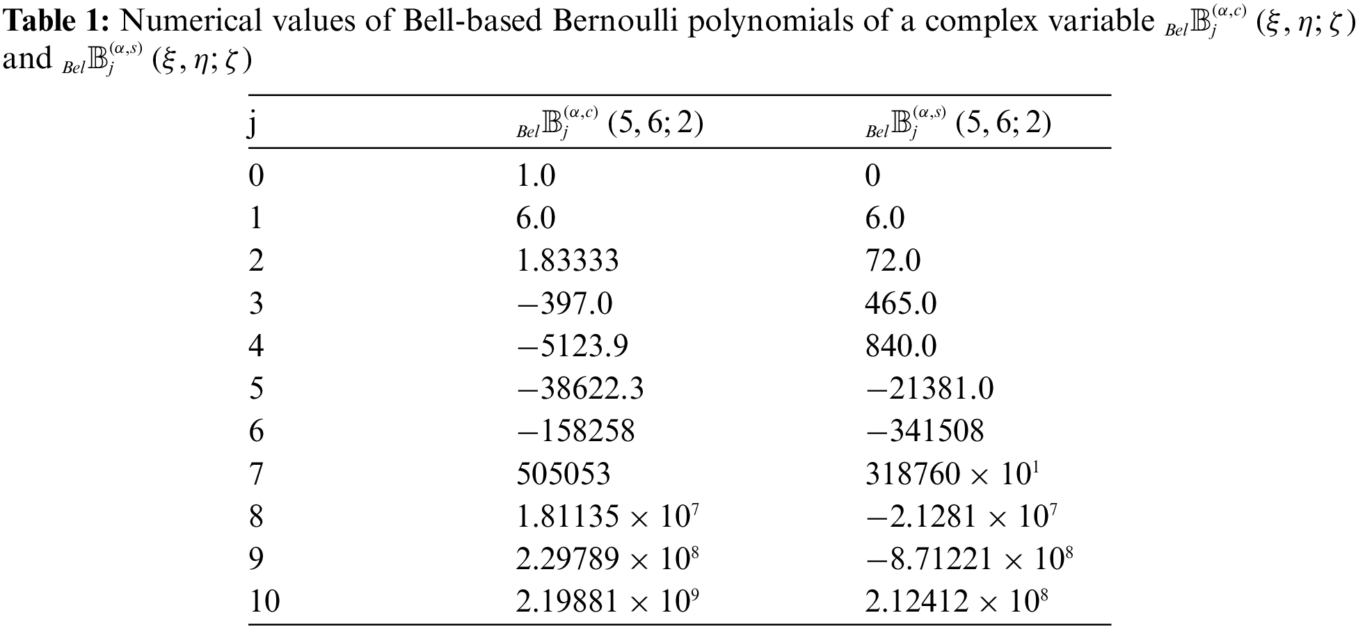
Fig. 1 shows the plot for the Bell-based Bernoulli polynomial $BelBj(α,c)(ξ,η;ζ)$ with $(ξ,η;ζ)=(5,6;2)$ . Fig. 2 shows the plot for 3D Bell-based Bernoulli polynomials $BelBj(α,c)(ξ,η;ζ)$ .

images

Figure 1: Bell-based Bernoulli polynomials $BelBj(α,c)(ξ,η;ζ)$

images

Figure 2: 3D Bell-based Bernoulli polynomials $BelBj(α,c)(ξ,η;ζ)$

5 Computational Values and Graphical Representations of Bell-Based Euler Polynomials of Complex Variable

In this section, certain zeros of the Bell-based Bernoulli polynomials of complex variable $BelEj(α,c)(ξ,η;ζ)$ and $BelEj(α,s)(ξ,η;ζ)$ and beautifully graphical representations are shown.

The first few of them are

$BelE0(α,c)(ξ,η;ζ)=1,$

$BelE1(α,c)(ξ,η;ζ)=−α2+ζ+ξ,$

$BelE2(α,c)(ξ,η;ζ)=α24+ζ−η2+(ζ+ξ)2−14α(1+4ζ+4ξ),$

$BelE3(α,c)(ξ,η;ζ)=ζ−18(α−2(ζ+ξ))(α2+12(ζ−η2))+4(ζ+ξ)2−α(3+4ζ+4ξ),$

$BelE4(α,c)(ξ,η;ζ)=−116(α2−2α3(3+4ζ+4ξ))+3α2(1+8ζ2−8η2+16ζ(1+ξ)+8ξ(1+ξ))+16(ζ4+η4−6η2ξ2+ξ4+ξ3(6+4ξ)+ζ(1+2ξ)(1−6η2+2ξ(1+ξ)))+ζ2(7−6η2+6ξ(2+ξ))−2α(−1−12η2+4(4ζ3+3ζ2(5+4ξ))+ζ(7−12η2+6ξ(3+2ξ))+ξ(−12η2+ξ(3+4ξ))),$

$andBelE0(α,s)(ξ,η;ζ)=0,$

$BelE1(α,s)(ξ,η;ζ)=η,$

$BelE2(α,s)(ξ,η;ζ)=η(−α+2(ζ+ξ)),$

$BelE3(α,s)(ξ,η;ζ)=14η(12ζ−4η2+3(α2+4(ζ+ξ)2−α(1+4ζ+4ξ))),$

$BelE4(α,s)(ξ,η;ζ)=12η(8ζ−(α−2(ζ+ξ))(α2+12ζ−4η2)+4(ζ+ξ)2−α(3+4ζ+4ξ)).$

Table 2 shows some numerical values of Numerical values of Bell-based Euler polynomials of complex variable.

images

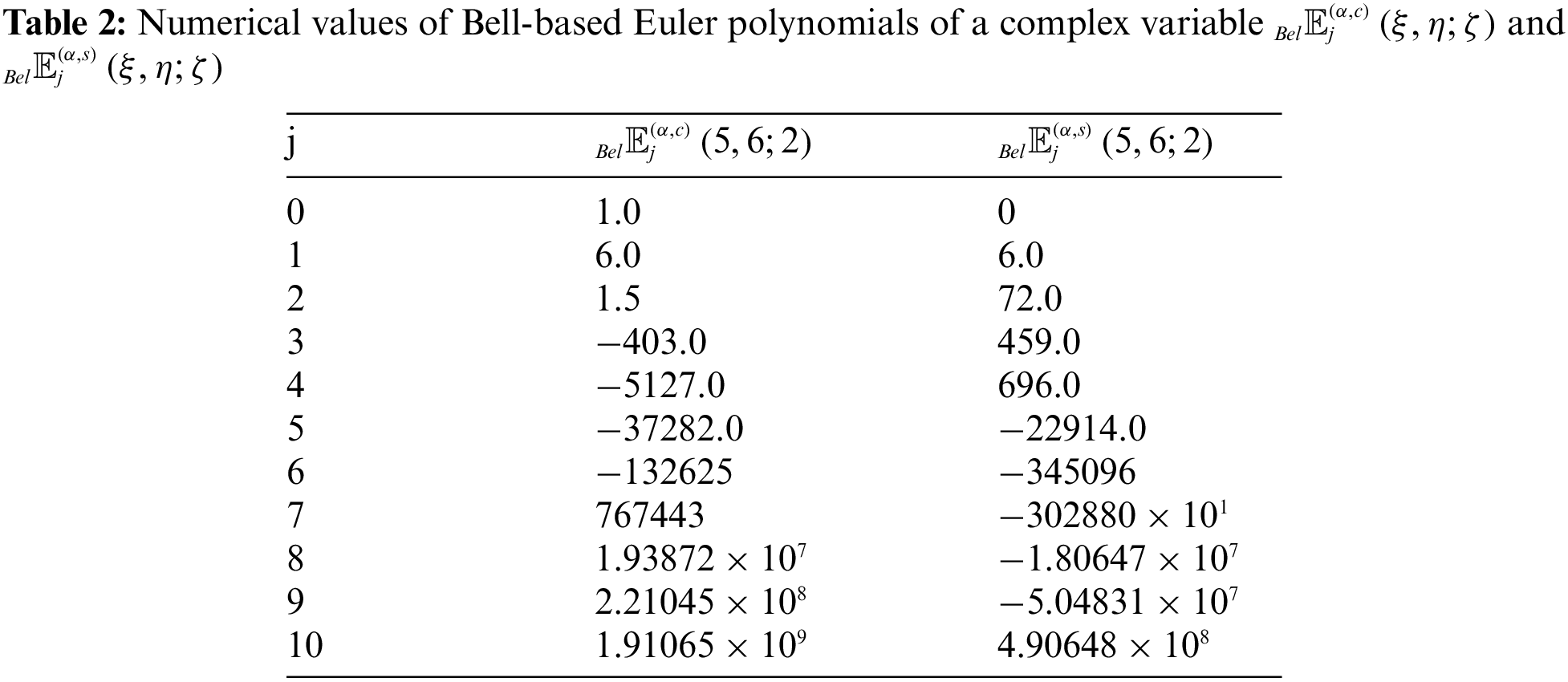
Fig. 3 shows the plot for the Bell-based Euler polynomial $BelEj(α,c)(ξ,η;ζ)$ with $(ξ,η;ζ)=(5,6;2)$ .

images

Figure 3: Bell-based Euler polynomials $BelBj(α,c)(ξ,η;ζ)$

6 Conclusions

In the present article, we have considered the parametric kinds of Bell-based Bernoulli and Euler polynomials by making use of the exponential as well as trigonometric functions. We have also derived some analytical properties of our newly introduced parametric polynomials by using the series manipulation technique. Furthermore, it is noticed that, if we consider any Appell polynomials of a complex variable (as discussed in the present article), then we can easily define its parametric kinds by separating the complex variable into real and imaginary parts. Consequently, the results of this article may potentially be used in mathematics, mathematical physics and engineering.

Acknowledgement: The authors wish to express their appreciation to the reviewers for their helpful suggestions which greatly improved the presentation of this paper.

Funding Statement: This research was funded by Research Deanship at the University of Ha’il, Saudi Arabia, through Project No. RG-21 144.

Conflicts of Interest: The authors declare that they have no conflicts of interest to report regarding the present study.

References

1. Avram, F., Taqqu, M. S. (1987). Noncentral limit theorems and Appell polynomials. The Annals of Probability, 15(2), 767–775. DOI 10.1214/aop/1176992170. [Google Scholar] [CrossRef]

2. Duran, U., Mehmet, A., Araci, S. (2021). Bell-based Bernoulli polynomials. Axioms, 10(29), 1–23. DOI 10.3390/axioms10010029. [Google Scholar] [CrossRef]

3. Hussain, S. S., Muhiuddin, G., Durga, N., Al-Kadi, D. (2022). New concepts on quadripartioned bipolar single valued neutrosophic graph. Computer Modeling in Engineering & Sciences, 130(1), 559–580. DOI 10.32604/cmes.2022.017032. [Google Scholar] [CrossRef]

4. Jamei, M. M., Beyki, M. R., Koepf, W. (2018). A new type of Euler polynomials and numbers. Mediterranean Journal of Mathematics, 15(138), 1–17. DOI 10.1007/s00009-018-1181-1. [Google Scholar] [CrossRef]

5. Jamei, M. M., Beyki, M. R., Koepf, W. (2017). Symbolic computation of some power trigonometric series. Journal of Symbolic Computation, 80, 273–284. DOI 10.1016/j.jsc.2016.03.004. [Google Scholar] [CrossRef]

6. Khan, W. A., Muhiuddin, G., Muhyi, A., Al-Kadi, D. (2021). Analytical properties of type 2 degenerate poly-Bernoulli polynomials associated with their applications. Advances in Difference Equations, 2021(1), 420. DOI 10.1186/s13662-021-03575-7. [Google Scholar] [CrossRef]

7. Kim, D. S., Kim, T. (2015). Some identities of Bell polynomials. Science China Mathematics, 58(10), 1–10. DOI 10.1007/s11425-015-5006-4. [Google Scholar] [CrossRef]

8. Muhiuddin, G., Khan, W. A., Duran, D., Al-Kadi, D. (2021). Some identities of the multi poly-Bernoulli polynomials of complex variable. Journal of Function Spaces, 2021(2), 1–8. DOI 10.1155/2021/7172054. [Google Scholar] [CrossRef]

9. Muhiuddin, G., Khan, W. A., Al-Kadi, D. (2021). Construction on the degenerate poly-Frobenius-Euler polynomials of complex variable. Journal of Function Spaces, 2021(1), 1–9. DOI 10.1155/2021/3115424. [Google Scholar] [CrossRef]

10. Muhiuddin, G., Khan, W. A., Muhyi, A., Al-Kadi, D. (2021). Some results on type 2 degenerate poly-Fubini polynomials and numbers. Computer Modeling in Engineering & Sciences, 129(2), 1051–1073. DOI 10.32604/cmes.2021.016546. [Google Scholar] [CrossRef]

11. Muhiuddin, G., Khan, W. A., Younis, J. (2021). Construction of type 2 poly-Changhee polynomials and its applications. Journal of Mathematics, 2021(4), 1–9. DOI 10.1155/2021/7167633. [Google Scholar] [CrossRef]

12. Khan, W. A., Ali, R., Alzobydi, K. A. H., Ahmad, N. (2021). A new family of degenerate poly-Genocchi polynomials with its certain properties. Journal of Function Spaces, 2021(4), 1–8. DOI 10.1155/2021/6660517. [Google Scholar] [CrossRef]

13. Kim, T., Ryoo, C. S. (2018). Some identities for Euler and Bernoulli polynomials and their zeros. Axioms, 7(3), 56. DOI 10.3390/axioms7030056. [Google Scholar] [CrossRef]

14. Kim, T., Khan, W. A., Sharma, S. K., Ghayasuddin, M. (2020). A note on parametric kinds of the degenerate poly-Bernoulli and poly-Genocchi polynomials. Symmetry, 12(4), 614. DOI 10.3390/sym12040614. [Google Scholar] [CrossRef]

15. Kim, T., Ryoo, C. S. (2019). Sheffer type degenerate Euler and Bernoulli polynomials. Filomat, 33(19), 6173–6185. DOI 10.2298/FIL1919173K. [Google Scholar] [CrossRef]

16. Kim, D. S., Kim, T., Lee, H. (2019). A note on degenerate Euler and Bernoulli polynomials of complex variables. Symmetry, 11(9), 1168. DOI 10.3390/sym11091168. [Google Scholar] [CrossRef]

17. Kim, D. S., Kim, T. (2021). Some identities on truncated polynomials associated with degenerate Bell polynomials. Russian Journal of Mathematical Physics, 28(3), 342–355. DOI 10.1134/S1061920821030079. [Google Scholar] [CrossRef]

18. Khan, W. A., Kamarujjama, M., Daud (2022). Construction of partially degenerate Bell-Bernoulli polynomials of the first kind and its certain properties. Analysis. https://www.degruyter.com/journal/key/anly/html?lang=en. [Google Scholar]

19. Ryoo, C. S., Khan, W. A. (2020). On two bivariate kinds of poly-Bernoulli and poly-Genocchi polynomials. Mathematics, 8(3), 417. DOI 10.3390/math8030417. [Google Scholar] [CrossRef]

20. Sharma, S. K., Khan, W. A., Ryoo, C. S. (2020). A parametric kind of the degenerate Fubini numbers and polynomials. Mathematics, 8(3), 405. DOI 10.3390/math8030405. [Google Scholar] [CrossRef]

21. Sharma, S. K., Khan, W. A., Ryoo, C. S. (2020). A parametric kind of Fubini polynomials of a complex variable. Mathematics, 8, 643. DOI 10.3390/math8040643./1.5114093. [Google Scholar] [CrossRef]

22. Tempesta, P. (2007). Formal groups, Bernoulli type polynomial and L-series. Comptes Rendus Mathematique, 345(6), 303–306. DOI 10.1016/j.crma.2007.05.016. [Google Scholar] [CrossRef]

Cite This Article

APA Style

Alam, N., Khan, W.A., Obeidat, S., Muhiuddin, G., Diab, N.S. et al. (2023). A Note on Bell-Based Bernoulli and Euler Polynomials of Complex Variable. Computer Modeling in Engineering & Sciences, 135(1), 187–209. https://doi.org/10.32604/cmes.2022.021418

Vancouver Style

Alam N, Khan WA, Obeidat S, Muhiuddin G, Diab NS, Zaidi HN, et al. A Note on Bell-Based Bernoulli and Euler Polynomials of Complex Variable. Comput Model Eng Sci. 2023;135(1):187–209. https://doi.org/10.32604/cmes.2022.021418

IEEE Style

N. Alam et al., “A Note on Bell-Based Bernoulli and Euler Polynomials of Complex Variable,” Comput. Model. Eng. Sci., vol. 135, no. 1, pp. 187–209, 2023. https://doi.org/10.32604/cmes.2022.021418

BibTex EndNote RIS

Copyright © 2023 The Author(s). Published by Tech Science Press.
This work is licensed under a Creative Commons Attribution 4.0 International License , which permits unrestricted use, distribution, and reproduction in any medium, provided the original work is properly cited.

Table of Content

A Note on Bell-Based Bernoulli and Euler Polynomials of Complex Variable

Abstract

Keywords

References

Cite This Article

1297

795

0

Related articles

Further Information

Guidelines

Follow Us

Join Us

Share Link