
 Submit a Paper
 Propose a Special lssue
 Open Access
ARTICLE
The Fractional Investigation of Fornberg-Whitham Equation Using an Efficient Technique
1 Department of Mathematics, Abdul Wali Khan University, Mardan, 23200, Pakistan
2 Department of Mathematics, Near East University TRNC, Mersin, 10, Turkey
3 Center of Excellence in Theoretical and Computational Science (TaCS-CoE) & KMUTTFixed Point Research
Laboratory, Room SCL 802 Fixed Point Laboratory, Science Laboratory Building, Departments of Mathematics, Faculty of Science, King Mongkut's University of Technology Thonburi (KMUTT), Bangkok, 10140, Thailand
4 Department of Medical Research, China Medical University Hospital, China Medical University, Taichung, 40402, Taiwan
* Corresponding Author: Poom Kumam. Email:
Computer Modeling in Engineering & Sciences 2023, 135(1), 259-273. https://doi.org/10.32604/cmes.2022.021332
Received 09 January 2022; Accepted 17 May 2022; Issue published 29 September 2022
 View Full Text
 Download PDF
Abstract
In the last few decades, it has become increasingly clear that fractional calculus always plays a very significant role in various branches of applied sciences. For this reason, fractional partial differential equations (FPDEs) are of more importance to model the different physical processes in nature more accurately. Therefore, the analytical or numerical solutions to these problems are taken into serious consideration and several techniques or algorithms have been developed for their solution. In the current work, the idea of fractional calculus has been used, and fractional Fornberg Whitham equation (FFWE) is represented in its fractional view analysis. A well-known method which is residual power series method (RPSM), is then implemented to solve FFWE. The RPSM results are discussed through graphs and tables which conform to the higher accuracy of the proposed technique. The solutions at different fractional orders are obtained and shown to be convergent toward an integer-order solution. Because the RPSM procedure is simple and straightforward, it can be extended to solve other FPDEs and their systems.Keywords
In mathematical physics, the Fornberg-Whitham equation is a fundamental mathematical model. The Fornberg-Whitham equation [1,2] is written as:
This equation was introduced to investigate how non-linear dispersive water waves break. The Fornberg-Whitham equation is shown to allow peakon solutions, as well as the occurrence of wave breaking, as a mathematical model for waves of limiting height. Fractional calculus (FC) is now widely used and accepted, owing to its well-established applications in a wide range of seemingly disparate domains of science and engineering [3–7]. Many scholars, including Gupta et al. [8], Merdan et al. [9], Singh et al. [10], have examined the fractional extension of the Fornberg-Whitham equation relevant to the Caputo fractional derivative.
FC has the potential to explain various difficult phenomena like memory and heredity. In recent years, researchers have taken a keen interest in the subject of fractional differential equations (FDEs), such as viscoelasticity, fluid mechanics, nanotechnology, electrochemistry, modelling for shape memory polymers, biological population models, optics and signal processing, modelling control theory, the damping behaviour of materials, economics and chemistry, signal processing, creeping and relaxation for viscoelastic materials and diffusion and reaction processes [11–13]. Accurate modelling of time-fractional two-mode coupled burgers equation is done with the help of fractional derivatives (FD) [14].
Analytical and numerical techniques are frequently used for the solution of FPDEs and their systems. The fractional problems that have been modelled by using FPDEs are found in various disciplines, because the mathematical modelling of real-life phenomena is usually modelled accurately by using FPDEs.
In this connection, the important fractional mathematical models are solved by using various techniques such as Chun-hui He’s algorithm [15], reproducing kernel method [16], Runge-Kutta method for time discretization and Fourier transform for spatial discretization [17], Fourier spectral method [18], He-Laplace method [19], Fractional variational iteration method [20], operational matrix of fractional Riemann-Liouville integration with Legendre basis and zeros of Chebyshev polynomials [21]. Khan et al. [22] have solved nonlinear fractional differential equations using an efficient approach. The non-linear differential equations are solved by using perturbation transform method and He’s polynomials [23]. The one-dimensional non-homogeneous partial differential equations with a variable coefficient are solved by using homotopy perturbation method and Laplace transformation [24]. Linear and non-linear differential equations arising in circuit analysis are investigated by using Maclaurin series method [25]. The analysis of Caputo fractional-order dynamics of Middle East Lungs Coronavirus (MERS-CoV) model are discussed in [26]. He’s fractional derivative and fractional complex transform are implemented for the time fractional Camassa-Holm equation [27]. The fractional complex transform is utilised to solve time-fractional Schr
Many researchers have worked hard to find the solutions to FPDEs by using RPSM and other novel techniques that have been used for the solutions of FPDEs like: Senol et al. [38] solved the time-fractional nonlinear coupled Jaulent-Miodek system with energy-dependent Schrodinger Potential using RPSM in 2019, Korpinar et al. [39] have analysed the solution of the fractional cancer model by RPSM, Kurt [40] has implemented RPSM to obtain the solution of fractional Bogoyavlensky-Konopelchenko equation, Xu et al. [41] have implemented RPSM to obtain the solution of fractional Boussinesq equations, Freihet et al. [42] have found the solution of fractional Burgers-Huxley equations in by using RPSM. Jena et al. [43] have found the solution of the fractional model of the vibration equation of large membranes using RPSM.
In the current work, the solution of FFWE is investigated by RPSM. The RPSM was found to be a very effective technique for finding the analytical solution of FFWE [44]. In the current work, we have applied the RPSM technique to solve different FPDEs and obtained the series form solutions. The closed form series solution is achieved for FFWE by using the proposed analytical technique. The accuracy of RPSM is represented by using graphs and tables. The solutions at different fractional orders are of greater interest, which show the useful information about the actual dynamics of the given problems. The graphs show the convergence of fractional solutions of the targeted problem towards integer order solution. The proposed method is also applied to other physical problems in applied sciences and engineering. The article layout is organized as follows; the fundamental concepts regarding FC are described in Section 2; the basic methodology is discussed in Section 3; the application of RPSM in the Fornberg-Whitham equation involving the Caputo fractional derivative is contained in Section 4; results and discussion are in Section 5 and the conclusion is given in Section 6.
In this section, we discussed some preliminaries and definitions.
The integral operator of Reimann-Liouville having order
Its fractional derivative for
where m is an integer.
The Caputo FD operator of the fractional order
The operators
•
•
•
•
•
A Power Series (PS) expansion is defined as [47]:
Theorem
Assume that
If
To the understand the procedure of RPSM [49–54], let consider FPDEs of the form
having initial condition,
where
the
Let uk(
exchange the
Also obtain
4 Solution of Time-Fractional F-W Equation
Let us consider the time fractional F-W equation,
with initial condition,
Let
We define the
As
For the first step,
Now we can write Eq. (7), for
Differentiating of Eq. (10), and put Eq. (9), we have
from Eq. (11), and
therefore
then from Eq. (7), and Eq. (12), we get
using Eq. (6), put in Eq. (13), then we have
Step 2. for
Now we can written Eq. (7), for
Similarly,
applying
Now using Eq. (12) and Eq. (17), in Eq. (15), we get
Putting Eq. (6), and Eq. (12), in Eq. (18), we have
For the third step, putting
From Eq. (7), put
same as the above procedure
Applying
therefore
Using Eq. (6), Eq. (12), and Eq. (18), put in Eq. (22), we have
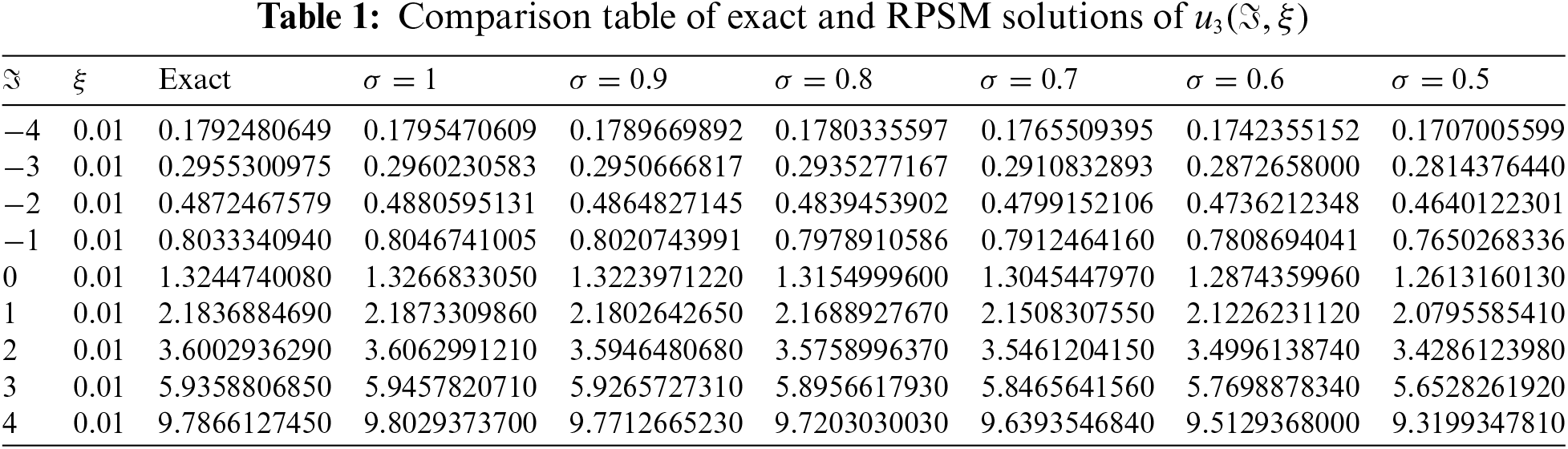
Equivalence of the 3rd-order approximate solution of
In Fig. 1, the exact and RPSM solutions at
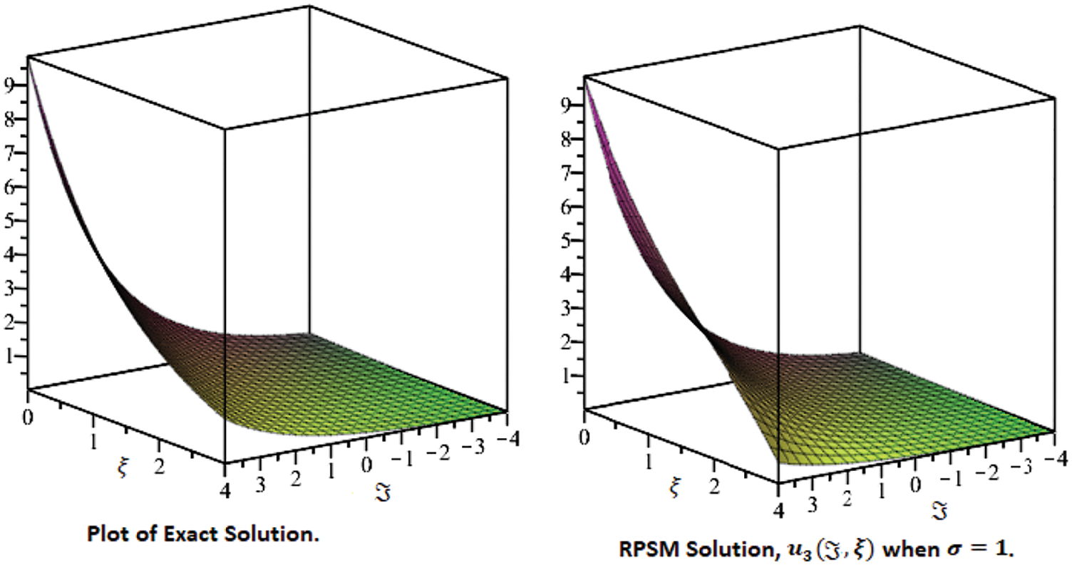
Figure 1: Comparison plots of exact and approximate solutions at the fractional order σ = 1
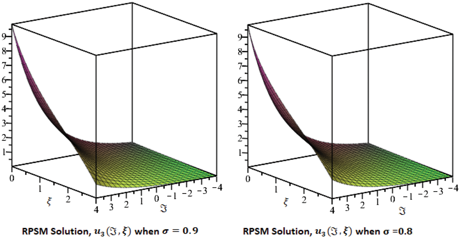
Figure 2: Comparison plots of approximate solutions at the fractional order σ = 0.9 and σ = 0.8
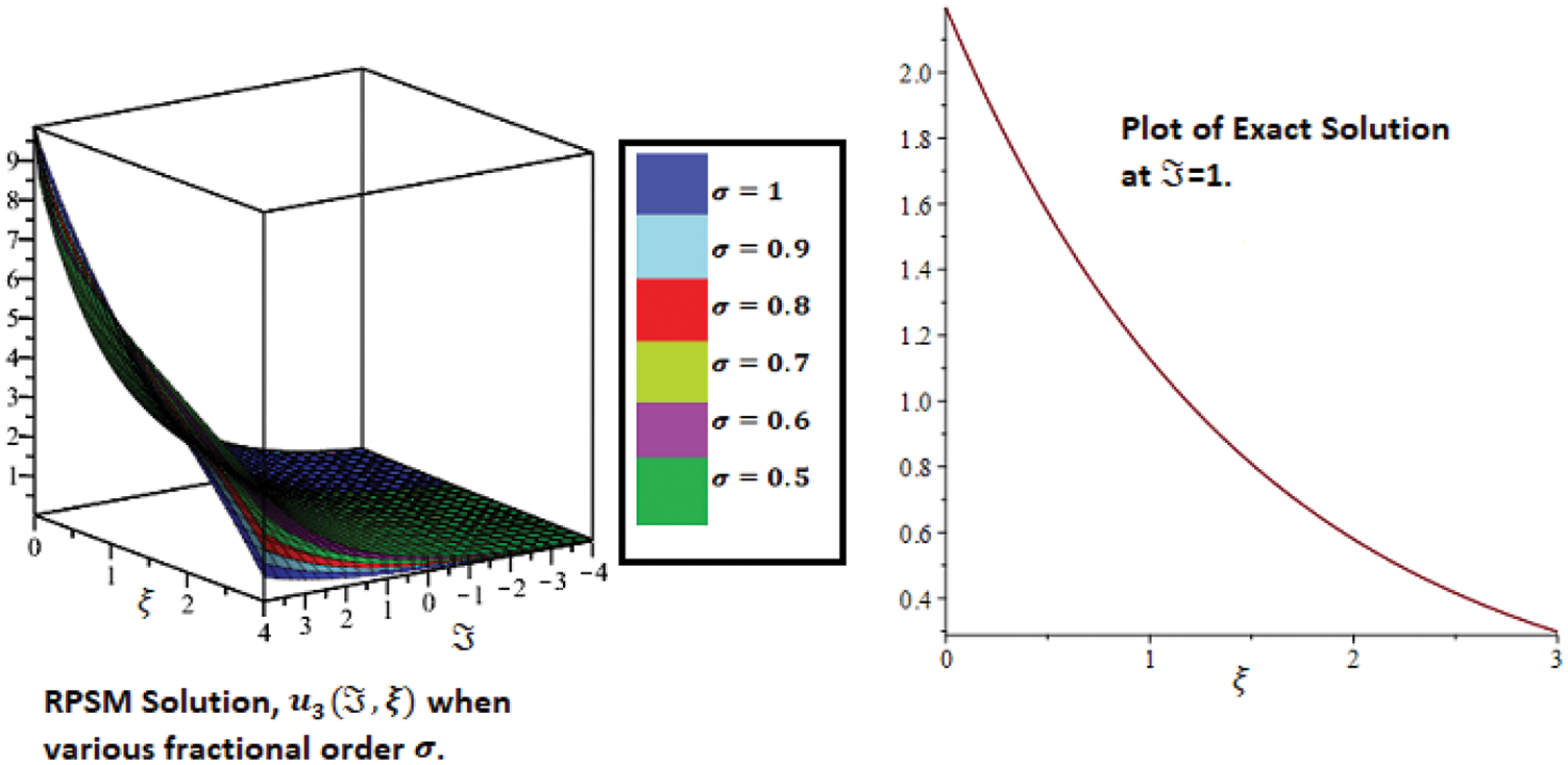
Figure 3: Combine 3D graphs for different fractional orders σ and exact solution of 2D plot
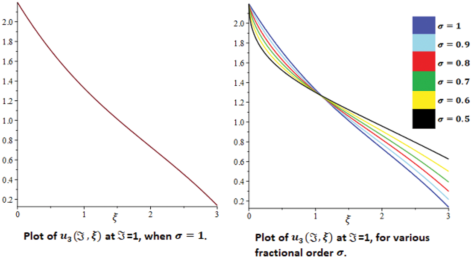
Figure 4: 2D plot and combine plot for various fractional order σ
Table 1 lists the result of RPSM
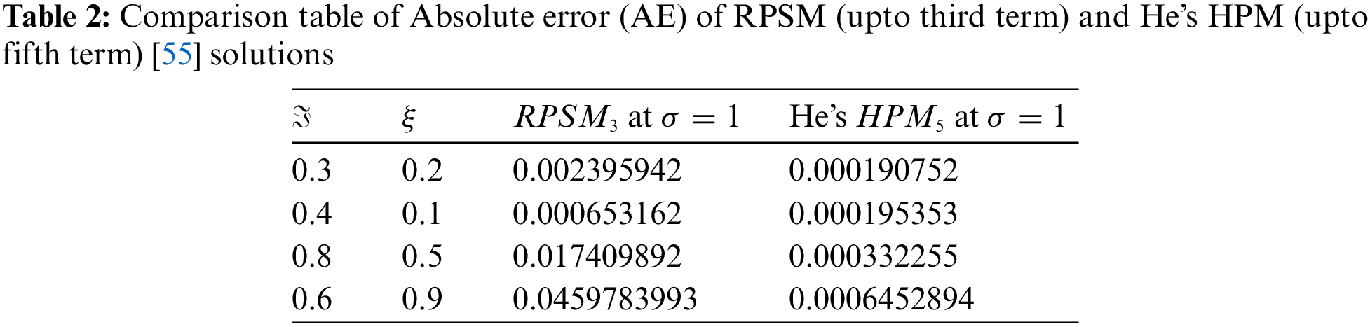
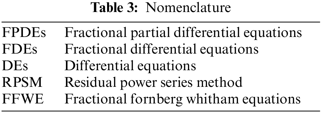
In Table 2, the solutions comparison of RPSM with He’s HPM is discussed. It is analyzed that the RPSM solution up to three terms is quite closed to the He’s HPM solutions which is calculated up to five terms. The tables and graphs have confirmed the higher degree of accuracy of RPSM. In Table 3, some nomenclatures are given which are frequently used in this paper.
In this work, we have implemented an efficient analytical technique, which is known as RPSM, to get an approximate series solution of FFWE with initial conditions. The suggested problems are first converted into their fractional form of the derivative and then incorporated the Caputo definition into the given problem to define FD. The general formulation for the proposed problem is discussed and then implemented for the solutions of FFWE. The proposed technique is applied to both fractional and integer orders of the suggested problem. It is observed that the procedure of the present technique is very effective and straight-forward. For verification and a better understanding of the obtained solutions, the graphical and tabular scenarios are presented. In Figs. 1–3, the exact and approximate solutions of the problem are presented, respectively. The solution graphs are presented at different fractional orders of the derivatives and show the various useful dynamics of the problem. It is investigated through numerical results and graphs that the fractional solutions are convergent to the integer-order solution. The analysis has shown the best contact between the RPSM and the exact solutions to the problem. For this purpose, the 2D graphs are discussed through Graphs 3 and 4. The 2D graphs clearly indicate that the proposed technique provides sufficient accuracy for problems with fractional orders. On the basis of the above analysis, it can be concluded that the proposed technique can be expanded easily to solve other problems in science and engineering. The values of the exact and approximate solutions of various fractional orders of the proposed method are given in Table 1, respectively. The exact and RPSM solution analyses given in Table 1 confirmed the higher accuracy.
Authors Contribution: Hassan Khan (Supervision), Poom Kumam (Funding, Draft Writing), Asif Nawaz (Methodology), Qasim Khan (Methodology, Investigation), Shahbaz Khan (Draft Writing).
Availability of Data and Material: Not applicable.
Funding Statement: The authors acknowledge the financial support provided by the Center of Excellence in Theoretical and Computational Science (TaCS-CoE), KMUTT. This research project is supported by Thailand Science Research and Innovation (TSRI) Basic Research Fund: Fiscal year 2022 under Project No. FRB650048/0164.
Conflicts of Interest: The authors declare that they have no conflicts of interest to report regarding the present study.
References
1. Jimenez, J., Whitham, G. B. (1976). An averaged lagrangian method for dissipative wavetrains. Proceedings of the Royal Society. A. Mathematical and Physical Sciences, 349(1658), 277–287. London. [Google Scholar]
2. Fornberg, B., Whitham, G. B. (1978). A numerical and theoretical study of certain nonlinear wave phenomena. philosophical transactions of the royal society of London. series A. Mathematical and Physical Sciences, 289(1361), 373–404. [Google Scholar]
3. Miller, K. S., Ross, B. (1993). An Introduction to the fractional calculus and fractional differential equations. New York: Wiley. [Google Scholar]
4. Debnath, L. (2003). Fractional integral and fractional differential equations in fluid mechanics. Fractional Calculus and Applied Analysis, 6(2), 119–155. [Google Scholar]
5. Caputo, M. (1969). Elasticita e dissipazione. Italy: Zanichelli. [Google Scholar]
6. Singh, J., Kumar, D., Nieto, J. J. (2016). A reliable algorithm for a local fractional tricomi equation arising in fractal transonic flow. Entropy, 18(6), 206. DOI 10.3390/e18060206. [Google Scholar] [CrossRef]
7. Srivastava, H. M., Kumar, D., Singh, J. (2017). An efficient analytical technique for fractional model of vibration equation. Applied Mathematical Modelling, 45, 192–204. DOI 10.1016/j.apm.2016.12.008. [Google Scholar] [CrossRef]
8. Gupta, P. K., Singh, M. (2011). Homotopy perturbation method for fractional Fornberg-Whitham equation. Computers & Mathematics with Applications, 61(2), 250–254. DOI 10.1016/j.camwa.2010.10.045. [Google Scholar] [CrossRef]
9. Merdan, M., Gökdoğan, A., Yildirim, A., Mohyud-Din, S. T. (2012). Numerical simulation of fractional Fornberg-Whitham equation by differential transformation method. In: Abstract and applied analysis, vol. 2012. Hindawi. [Google Scholar]
10. Singh, J., Kumar, D., Kumar, S. (2013). New treatment of fractional Fornberg−Whitham equation via Laplace transform. Ain Shams Engineering Journal, 4(3), 557–562. [Google Scholar]
11. Neirameh, A., (2018). New fractional calculus and application to the fractional-order of extended biological population model. Boletim da Sociedade Paranaense de Matemática, 36(3), 115–128. DOI 10.5269/2175-1188. [Google Scholar] [CrossRef]
12. Cao, K., Chen, Y. (2018). Fractional order crowd dynamics. De Gruyter, 4. DOI 10.1515/9783110473988. [Google Scholar] [CrossRef]
13. Luchko, Y., Yamamoto, M. (2016). General time-fractional diffusion equation: Some uniqueness and existence results for the initial-boundary-value problems. Fractional Calculus and Applied Analysis, 19(3), 676–695. DOI 10.1515/fca-2016-0036. [Google Scholar] [CrossRef]
14. Shokhanda, R., Goswami, P., He, J. H., Althobaiti, A. (2021). An approximate solution of the time-fractional two-mode coupled burgers equation. Fractal and Fractional, 5(4), 196. DOI 10.3390/fractalfract5040196. [Google Scholar] [CrossRef]
15. He, C. H. (2016). An introduction to an ancient Chinese algorithm and its modification. International Journal of Numerical Methods for Heat & Fluid Flow, 26(8), 2486–2491. DOI 10.1108/HFF-09-2015-0377. [Google Scholar] [CrossRef]
16. Dai, D. D. (2021). The piecewise reproducing kernel method for the time variable fractional order advection-reaction-diffusion equations. Thermal Science, 25, 1261–1268. [Google Scholar]
17. Han, C., Wang, Y. L., Li, Z. Y. (2022). A high-precision numerical approach to solving space fractional gray-scott model. Applied Mathematics Letters, 125, 107759. DOI 10.1016/j.aml.2021.107759. [Google Scholar] [CrossRef]
18. Han, C., Wang, Y. L., Li, Z. Y. (2021). Numerical solutions of space fractional variable-coefficient KdV-modified KdV equation by Fourier spectral method. Fractals, 29(8), 2150246. DOI 10.1142/S0218348X21502467. [Google Scholar] [CrossRef]
19. He, J. H., Moatimid, G. M., Mostapha, D. R. (2021). Nonlinear instability of two streaming-superposed magnetic reiner-rivlin fluids by He-laplace method. Journal of Electroanalytical Chemistry, 895, 115388. DOI 10.1016/j.jelechem.2021.115388. [Google Scholar] [CrossRef]
20. Khan, Y., Faraz, N., Yildirim, A., Wu, Q. (2011). Fractional variational iteration method for fractional initial-boundary value problems arising in the application of nonlinear science. Computers & Mathematics with Applications, 62(5), 2273–2278. DOI 10.1016/j.camwa.2011.07.014. [Google Scholar] [CrossRef]
21. Khan, Y., Ali Beik, S. P., Sayevand, K., Shayganmanesh, A. (2015). A numerical scheme for solving differential equations with space and time-fractional coordinate derivatives. Quaestiones Mathematicae, 38(1), 41–55. DOI 10.2989/16073606.2014.981699. [Google Scholar] [CrossRef]
22. Khan, Y., Fardi, M., Sayevand, K., Ghasemi, M. (2014). Solution of nonlinear fractional differential equations using an efficient approach. Neural Computing and Applications, 24(1), 187–192. DOI 10.1007/s00521-012-1208-7. [Google Scholar] [CrossRef]
23. Khan, Y., Wu, Q. (2011). Homotopy perturbation transform method for nonlinear equations using He’s polynomials. Computers & Mathematics with Applications, 61(8), 1963–1967. DOI 10.1016/j.camwa.2010.08.022. [Google Scholar] [CrossRef]
24. Madani, M., Fathizadeh, M., Khan, Y., Yildirim, A. (2011). On the coupling of the homotopy perturbation method and laplace transformation. Mathematical and Computer Modelling, 53(9–10), 1937–1945. DOI 10.1016/j.mcm.2011.01.023. [Google Scholar] [CrossRef]
25. Khan, Y., Faraz, N. (2021). Simple use of the maclaurin series method for linear and non-linear differential equations arising in circuit analysis. COMPEL-The International Journal for Computation and Mathematics in Electrical and Electronic Engineering, 40(3), 593–601. DOI 10.1108/COMPEL-08-2020-0286. [Google Scholar] [CrossRef]
26. Ain, Q. T., Anjum, N., Din, A., Zeb, A., Djilali, S. et al. (2022). On the analysis of caputo fractional order dynamics of Middle East lungs coronavirus (MERS-CoV) model. Alexandria Engineering Journal, 61(7), 5123–5131. DOI 10.1016/j.aej.2021.10.016. [Google Scholar] [CrossRef]
27. Anjum, N., Ain, Q. T. (2020). Application of He’s fractional derivative and fractional complex transform for time fractional camassa-holm equation. Thermal Science, 24, 3023–3030. DOI 10.2298/TSCI190930450A. [Google Scholar] [CrossRef]
28. Ain, Q. T., He, J. H., Anjum, N., Ali, M. (2020). The fractional complex transform: A novel approach to the time-fractional Schrödinger equation. Fractals, 28(7), 2050141. DOI 10.1142/S0218348X20501418. [Google Scholar] [CrossRef]
29. Anjum, N., He, C. H., He, J. H. (2021). Two-scale fractal theory for the population dynamics. Fractals, 29(7), 2150182. DOI 10.1142/S0218348X21501826. [Google Scholar] [CrossRef]
30. Anjum, N., Ain, Q. T., Li, X. X. (2021). Two-scale mathematical model for Tsunami wave. GEM-International Journal on Geomathematics, 12(1), 1–12. DOI 10.1007/s13137-021-00177-z. [Google Scholar] [CrossRef]
31. El-Sayed, A. M. A., Nour, H. M., Raslan, W. E., El-Shazly, E. S. (2015). A study of projectile motion in a quadratic resistant medium via fractional differential transform method. Applied Mathematical Modelling, 39(10–11), 2829–2835. DOI 10.1016/j.apm.2014.10.018. [Google Scholar] [CrossRef]
32. Kumar, M., Rawat, T. K. (2015). Design of a variable fractional delay filter using comprehensive least square method encompassing all delay values. Journal of Circuits, Systems and Computers, 24(8), 1550116. DOI 10.1142/S0218126615501169. [Google Scholar] [CrossRef]
33. Alomari, A. K., Syam, M. I., Anakira, N. R., Jameel, A. F. (2020). Homotopy sumudu transform method for solving applications in physics. Results in Physics, 18, 103265. DOI 10.1016/j.rinp.2020.103265. [Google Scholar] [CrossRef]
34. Prakash, A., Veeresha, P., Prakasha, D. G., Goyal, M. (2019). A new efficient technique for solving fractional coupled Navier-Stokes equations using Q-homotopy analysis transform method. Pramana, 93(1), 1–10. DOI 10.1007/s12043-019-1763-x. [Google Scholar] [CrossRef]
35. Kocak, H., Pinar, Z. (2018). On solutions of the fifth-order dispersive equations with porous medium type non-linearity. Waves in Random and Complex Media, 28(3), 516–522. DOI 10.1080/17455030.2017.1367438. [Google Scholar] [CrossRef]
36. Momani, S., Odibat, Z. (2006). Analytical solution of a time-fractional navier-stokes equation by adomian decomposition method. Applied Mathematics and Computation, 177(2), 488–494. DOI 10.1016/j.amc.2005.11.025. [Google Scholar] [CrossRef]
37. Bayrak, M. A., Demir, A. (2018). A new approach for space-time fractional partial differential equations by residual power series method. Applied Mathematics and Computation, 336, 215–230. DOI 10.1016/j.amc.2018.04.032. [Google Scholar] [CrossRef]
38. Senol, M., Iyiola, O. S., Daei Kasmaei, H., Akinyemi, L. (2019). Efficient analytical techniques for solving time-fractional nonlinear coupled Jaulent-Miodek system with energy-dependent Schrödinger potential. Advances in Difference Equations, 2019(1), 1–21. [Google Scholar]
39. Korpinar, Z., Inc, M., Hinçal, E., Baleanu, D. (2020). Residual power series algorithm for fractional cancer tumor models. Alexandria Engineering Journal, 59(3), 1405–1412. DOI 10.1016/j.aej.2020.03.044. [Google Scholar] [CrossRef]
40. Kurt, A. (2020). New analytical and numerical results for fractional Bogoyavlensky-Konopelchenko equation arising in fluid dynamics. Applied Mathematics–A Journal of Chinese Universities, 35(1), 101–112. DOI 10.1007/s11766-020-3808-9. [Google Scholar] [CrossRef]
41. Xu, F., Gao, Y., Yang, X., Zhang, H. (2016). Construction of fractional power series solutions to fractional boussinesq equations using residual power series method. Mathematical Problems in Engineering, 2016, 1–15 DOI 10.1155/2016/5492535. [Google Scholar] [CrossRef]
42. Freihet, A. A., Zuriqat, M. (2019). Analytical solution of fractional burgers-huxley equations via residual power series method. Lobachevskii Journal of Mathematics, 40(2), 174–182. DOI 10.1134/S1995080219020082. [Google Scholar] [CrossRef]
43. Jena, R. M., Chakraverty, S. (2019). Residual power series method for solving time-fractional model of vibration equation of large membranes. Journal of Applied and Computational Mechanics, 5(4), 603–615. [Google Scholar]
44. Sakar, M. G., Erdogan, F., Yildirim, A. (2012). Variational iteration method for the time-fractional Fornberg-Whitham equation. Computers & Mathematics with Applications, 63(9), 1382–1388. DOI 10.1016/j.camwa.2012.01.031. [Google Scholar] [CrossRef]
45. Podlubny, I. (1998). Fractional differential equations: An introduction to fractional derivatives, fractional differential equations, to methods of their solution and some of their applications. USA: Academic Press. [Google Scholar]
46. Luchko, Y. F., Srivastava, H. M. (1995). The exact solution of certain differential equations of fractional order by using operational calculus. Computers & Mathematics with Applications, 29(8), 73–85. DOI 10.1016/0898-1221(95)00031-S. [Google Scholar] [CrossRef]
47. El-Ajou, A., Arqub, O. A., Momani, S. (2015). Approximate analytical solution of the nonlinear fractional KdV-burgers equation: A new iterative algorithm. Journal of Computational Physics, 293, 81–95. DOI 10.1016/j.jcp.2014.08.004. [Google Scholar] [CrossRef]
48. El-Ajou, A., Arqub, O. A., Zhour, Z. A., Momani, S. (2013). New results on fractional power series: Theories and applications. Entropy, 15(12), 5305–5323. DOI 10.3390/e15125305. [Google Scholar] [CrossRef]
49. Alquran, M. (2015). Analytical solution of time-fractional two-component evolutionary system of order 2 by residual power series method. Journal of Applied Analysis and Computation, 5(4), 589–599. DOI 10.11948/2015046. [Google Scholar] [CrossRef]
50. Alquran, M., Jaradat, H. M., Syam, M. I. (2017). Analytical solution of the time-fractional Phi-4 equation by using modified residual power series method. Nonlinear Dynamics, 90(4), 2525–2529. DOI 10.1007/s11071-017-3820-7. [Google Scholar] [CrossRef]
51. Freihet, A., Hasan, S., Al-Smadi, M., Gaith, M., Momani, S. (2019). Construction of fractional power series solutions to fractional stiff system using residual functions algorithm. Advances in Difference Equations, 2019(1), 95. [Google Scholar]
52. Hasan, S., Al-Smadi, M., Freihet, A., Momani, S. (2019). Two computational approaches for solving a fractional obstacle system in hilbert space. Advances in Difference Equations, 2019(1), 55. DOI 10.1186/s13662-019-1996-5. [Google Scholar] [CrossRef]
53. Prakasha, D. G., Veeresha, P., Baskonus, H. M. (2019). Residual power series method for fractional Swift-Hohenberg equation. Fractal and Fractional, 3(1), 9. DOI 10.3390/fractalfract3010009. [Google Scholar] [CrossRef]
54. Tchier, F., Inc, M., Korpinar, Z. S., Baleanu, D. (2016). Solutions of the time fractional reaction-diffusion equations with residual power series method. Advances in Mechanical Engineering, 8(10). DOI 10.1177/1687814016670867. [Google Scholar] [CrossRef]
55. Wang, K. L., Liu, S. Y. (2017). He’s fractional derivative and its application for fractional Fornberg-Whitham equation. Thermal Science, 21(5), 2049–2055. DOI 10.2298/TSCI151025054W. [Google Scholar] [CrossRef]
Cite This Article
 Copyright © 2023 The Author(s). Published by Tech Science Press.
This work is licensed under a Creative Commons Attribution 4.0 International License , which permits unrestricted use, distribution, and reproduction in any medium, provided the original work is properly cited.
 Downloads
 Citation Tools