Application of Automated Guided Vehicles in Smart Automated Warehouse Systems: A Survey

1  Introduction

Smart automated warehouse systems are important parts of the smart world, and the application of Automated Guided Vehicles (AGVs) is essential to applications in smart cities, and even more than 40% of its cost can be saved using AGVs. The application of AGVs in automated warehouses is both a management and a technology issue. The management issue refers to consider many experimental conditions, user demands, and environmental changes; the technology issue refers to make a tradeoff between quantity, quality, and efficiency. The application of AGVs has been widely studied.

AGVs have abilities of autonomous planning and coordination. AGVs systems can be classified into centralized and decentralized systems [1]. The centralized systems are convenient for applications, but may not work well in large environments. The decentralized systems work well in large environments, but the requirements of hardware and software are comparatively high. However, approximately 20%–50% of costs can be avoided by employing a practical warehouse layout and efficient work [2]. There are two types of materials flows in warehouses: receiving and delivering. The most time-consuming task is picking up goods (i.e., shelves). Reducing the travel time and system energy costs of AGVs is a critical problem for industries. However, in most publications, it failed to notice the problem of operation optimization in warehouse layout.

To complete an issued task, warehouses need to find an AGV that can reach the start node of the task as soon as possible. The period for an AGV moving to the start node is called the gap period. The shorter the gap period, the more efficient the warehouses. The objective of AGVs scheduling is to find an optimal AGV that can respond to the order as soon as possible [3]. Although there are many state-of-the-art methods related to AGVs scheduling [4,5], the performance of the algorithms in chessboard-like environments is rarely verified. Herein, we illustrated key models and present our ideas in detail.

AGVs route planning is both a single- and multi-objective optimization problem [6,7]. There are several requirements on such a route-planning algorithm: (a) shortest route, i.e., the length of the route should be minimized; (b) minimized time consumption, i.e., the system’s energy cost should be the least; (c) efficient route planning, i.e., the algorithm can compute an optimal route quickly in real-time. Although the classical AGVs route-planning algorithms (e.g., Dijkstra’s algorithm [8], A* algorithm [9], D* algorithm [10]) can work well in small warehouses, they could be inefficient in environments with many nodes. Recently, Artificial Intelligence (AI) has become a helpful tool in autonomous decision-making areas [11]. Reinforcement Learning (RL), more specifically, the Q-learning algorithm has shown significant advantages and has been used in route planning [12–14], but the convergence time is extended when the number of nodes becomes large. Although the importance of computation amount has been addressed in most publications, only a few effective policies were proposed in the regard of reducing the time of convergence. Here, we present a promising direction to shortening the iteration time of the Q-learning algorithm by integrating RL and Dijkstra’s algorithm.

The multi-AGV route planning belongs to the multi-agent path-finding problem [15], and its objective is to transport shelves to goal nodes without collisions while multiple AGVs travel together. The commonly used strategy for multi-AGV route planning is the prediction method [16], i.e., systems can detect whether the route conflicts exist or not by consulting AGVs’ planned routes and if they exist, the systems employ solutions to solve conflicts. However, most publications focus only on collisions avoidance effectiveness, ignoring the travel time and energy cost of AGV systems. With increased warehouses, the scenarios can be more complex (e.g., there are more nodes and uncertainties), but few publications comprehensively considered routes computation time, multi-AGV travel distance, multi-AGV travel time, energy cost, and dynamics of systems.

Many publications are related to the application of AGVs in smart automated warehouses, but few of them made systematic overviews of the problems in the real world. The following research contributions are made in this study:

1.    We attempted to fill the gap by addressing minor extent research on AGVs systems, warehouses layouts and operations optimization, AGVs scheduling, AGVs route planning, and some areas that have received little attention from researchers.

2.    The common layouts of warehouses (i.e., horizontal pattern, vertical pattern, and fish-bone pattern) are presented. Moreover, popular methods of modeling storage environments (e.g., topological map method, free space method, and grid method) are compared based on the characteristics of automated warehouses.

3.    Based on the classical AGVs scheduling methods, a novel idea of scheduling methods in chessboard-like warehouses is proposed, i.e., the method of adding penalty factors to the classical Dijkstra’s algorithm.

4.    The popular classical route-planning algorithms are presented and compared. Moreover, a novel AGVs route-planning method by combing the classical Dijkstra’s algorithm and the RL algorithm is proposed.

5.    Some promising research directions are presented after conducting the survey.

2  Motivation and Methodology

In this paper, we employed four filtering and analysis steps. (1) More than 300 related publications were analyzed from databases, such as Web of Science, Science Direct, Elsevier Digital Library, ACM Digital Library, and IEEE Explore. (2) Since some papers accessed above were behind a paywall, about 250 publications were obtained for further analysis and about 200 of them were related to the application of AGVs. (3) The abstracts and introductions of the remaining 200 publications were skimmed through. This was done to select the publications with the following demands: (a) they proposed efficient algorithms for AGVs scheduling or AGV route planning; (b) the environments are related to materials flow (e.g., automated warehouses or logistic industries); (c) the proposed algorithms could be implemented in realtime. Finally, the remaining 136 publications were read in detail and classified into four according to their characteristics. These publications were selected because they were involved in describing the future prospective of AGVs applications. Moreover, at the end of each part, we presented some of our standpoints for future research.

The rest of this paper is organized into Sections 3–7. In Section 3, we review the key publications related to AGVs systems. Based-on the review of the advantages and drawbacks of the centralized systems, it is concluded that AGVs can obtain more flexibility in the decentralized systems. In Section 4, we present several common warehouses layouts and storage allocation policies. Some easy-overlooked issues are also analyzed, e.g., the influence of electrical energy management and AGVs fleet size. In Section 5, several AGVs scheduling algorithms are reviewed, and a novel idea of scheduling AGVs in chessboard-like warehouses is proposed. In Section 6, the AGVs route-planning algorithms are presented, including the traditional and AI-based route-planning algorithms. In Section 7, we conclude the paper and point out the promising research directions for the future.

3  Establishment of AGVs Control Systems

3.1 Centralized Control Systems

The typical centralized AGVs systems are hierarchy systems, as shown in Fig. 1 [17]. The server has functions of supervising and decision-making, and the sub-system consists of many AGVs equipped with several independent models. The collision-free routes are computed using route-planning algorithms, then the planned routes are dispatched to every AGV, and the server will monitor every AGV’s traveling status, e.g., AGV’s location and electric energy, at the same time.

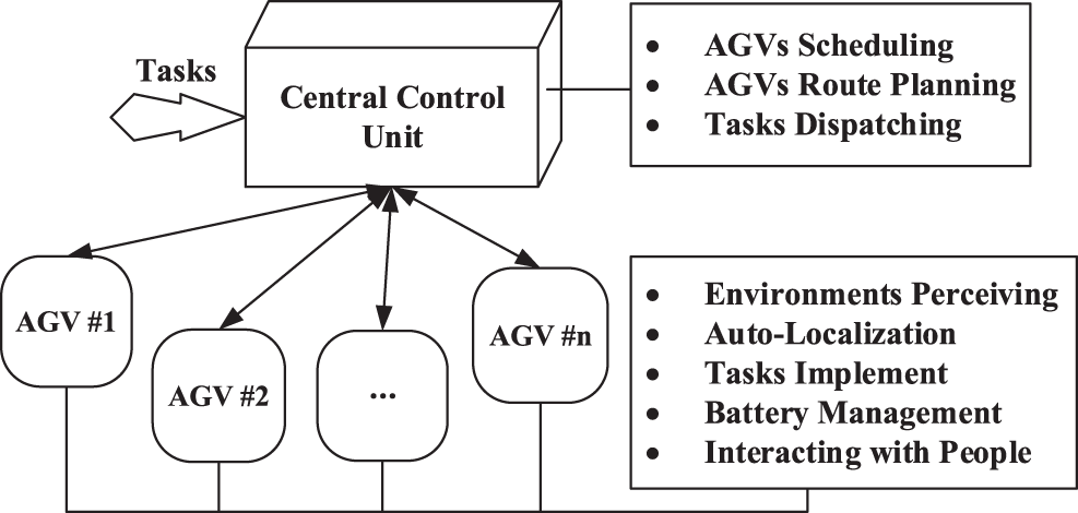
Figure 1: Centralized AGVs systems architecture

Since multiple AGVs are controlled by a server directly, the computational complexity of the server is large. Therefore, the decoupled operations are necessary [18–21], where the private zone mechanism-based coordination algorithm can satisfy the robustness under different collisions scenarios [22]. Moreover, it is necessary to employ effective information management methods to optimize the storage of goods, and the Intelligent & Agile Warehouse System (IAWS) can provide more flexible storage ways, increase accuracy and improve operation efficiency [23].

The advantages of centralized control systems are as follows [24]: (a) the global optimal solution can be obtained because routes are generated based on the global environments information; (b) it is robust and easy to follow in the real world because we needn’t equip computer on every AGV. On the other hand, the disadvantages are as follows [24]: (a) AGVs have limited autonomy; (b) the computation amount may be heavy in large-scale environments because the server should perform many complex tasks at the same time.

3.2 Decentralized Control Systems

The decentralized AGVs systems can provide a high level of autonomy since they are characterized by distributed computation, and the typical decentralized control systems are shown in Fig. 2 [1], where AGVs’ controllers can be divided into route-planning modules, which is responsible for computing the initial routes and the motion-coordinating modules, and motion coordination module, which is responsible for collision-free motions among AGVs. However, such decentralized systems were proposed based on unlimited environments, different from automated warehouses.

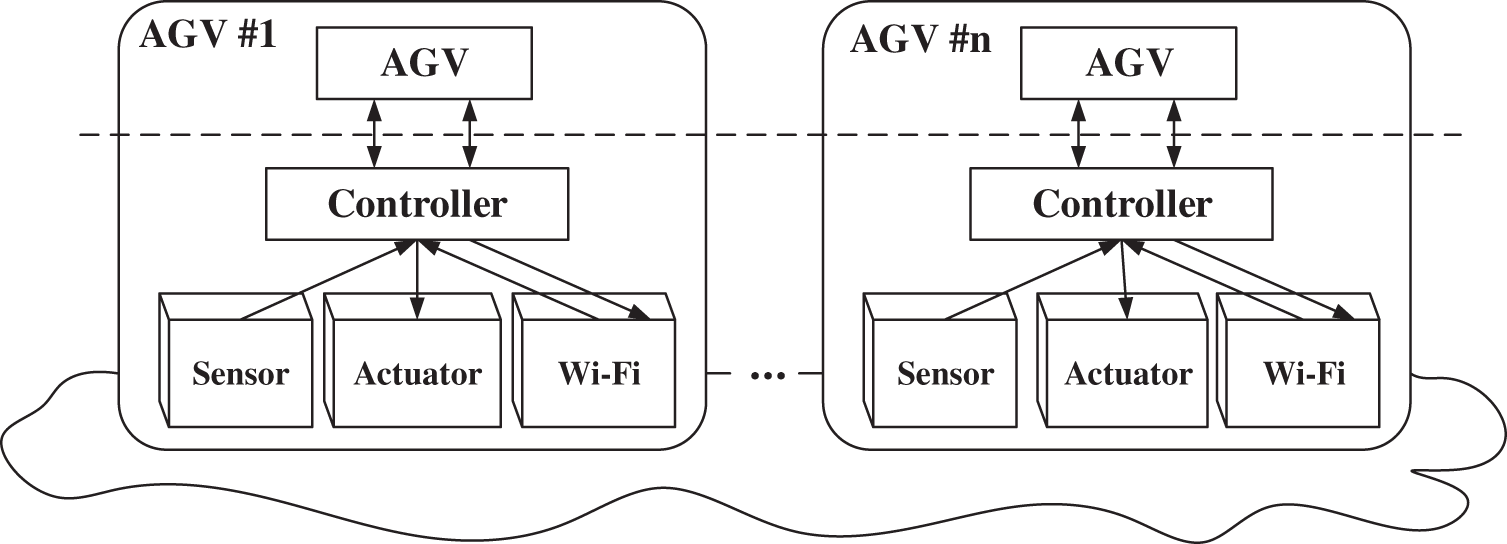
Figure 2: Decentralized control system architecture

The advantages of the decentralized systems are as follows [25]: (1) the data congestion could be avoided because every AGV can plan its route and just communicate with related AGVs instead of the server when conflicts occur; (2) they are easily scaled and can work well in large-scale environments. On the other hand, the disadvantages are as follows [25]: (1) it is a challenge to guarantee the optimal solution because AGVs can just obtain partial information about environments; (2) it has a high demand for hardware because every AGV should be equipped with a microcomputer.

4  Warehouse Layout and Operation Optimization

4.1 Environment Layout in Automated Warehouses

Without a proper layout, AGVs could not implement transportation tasks (i.e., shelf picking-up and delivery) efficiently. Several factors [26] that influence the automated warehouse layout as shown in Fig. 3.

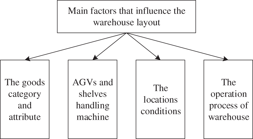
Figure 3: Factors that influence the automated warehouse layout

4.1.1 Paths Arrangement

There are three popular patterns for paths arrangement as shown in Fig. 4 [27,28]: (a) single one-way route pattern; (b) single two-way route pattern; (c) double one-way route pattern.

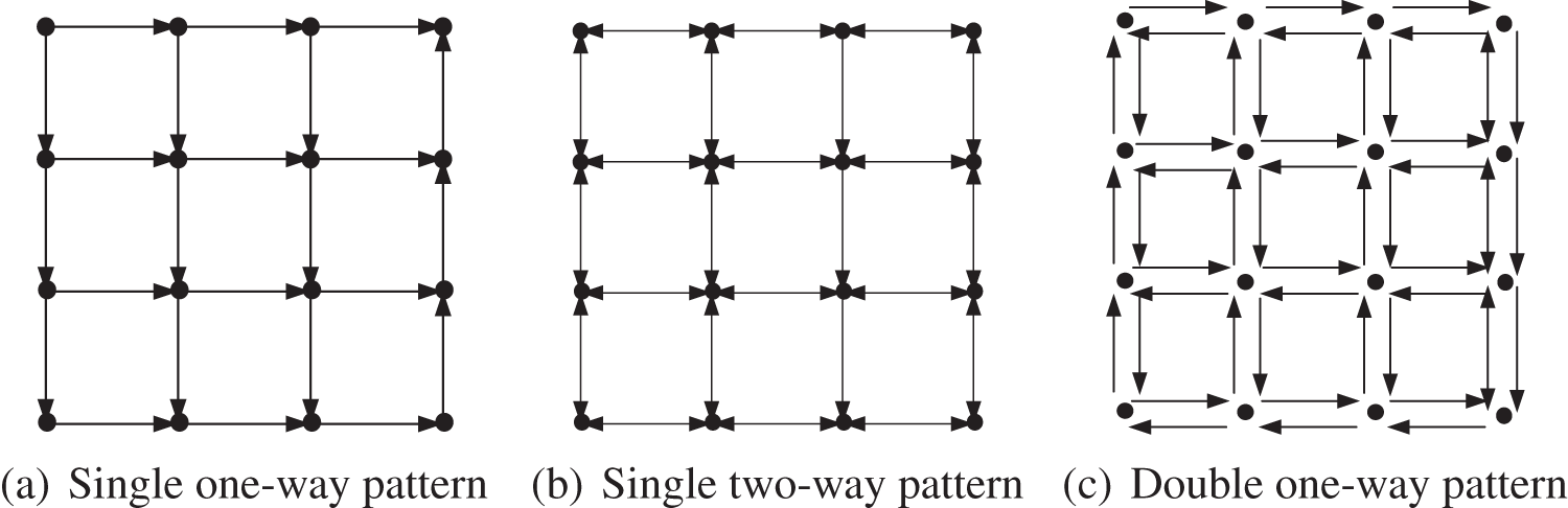
Figure 4: Common paths arrangement patterns

In the single one-way pattern, AGVs travel along with the exact directions, so the probability of collisions can be decreased significantly. However, it may reduce throughput because AGVs could not travel backward.

In the single two-way pattern, the flexibility of systems is improved since the map is bi-directional. However, the route planning becomes complicated because there may exist more types of collisions (e.g., head-on and cross-road collisions), and thus the probability of collisions is increased.

The double one-way pattern is the combination of the above two patterns. It brings benefits in regard of both systems’ flexibility and route-planning complicity. However, it needs more space to arrange workstations. Therefore, it is suitable for super-large-scale environments.

4.1.2 Facilities Arrangement

There are four popular warehouse layouts, as shown in Fig. 5 [29,30].

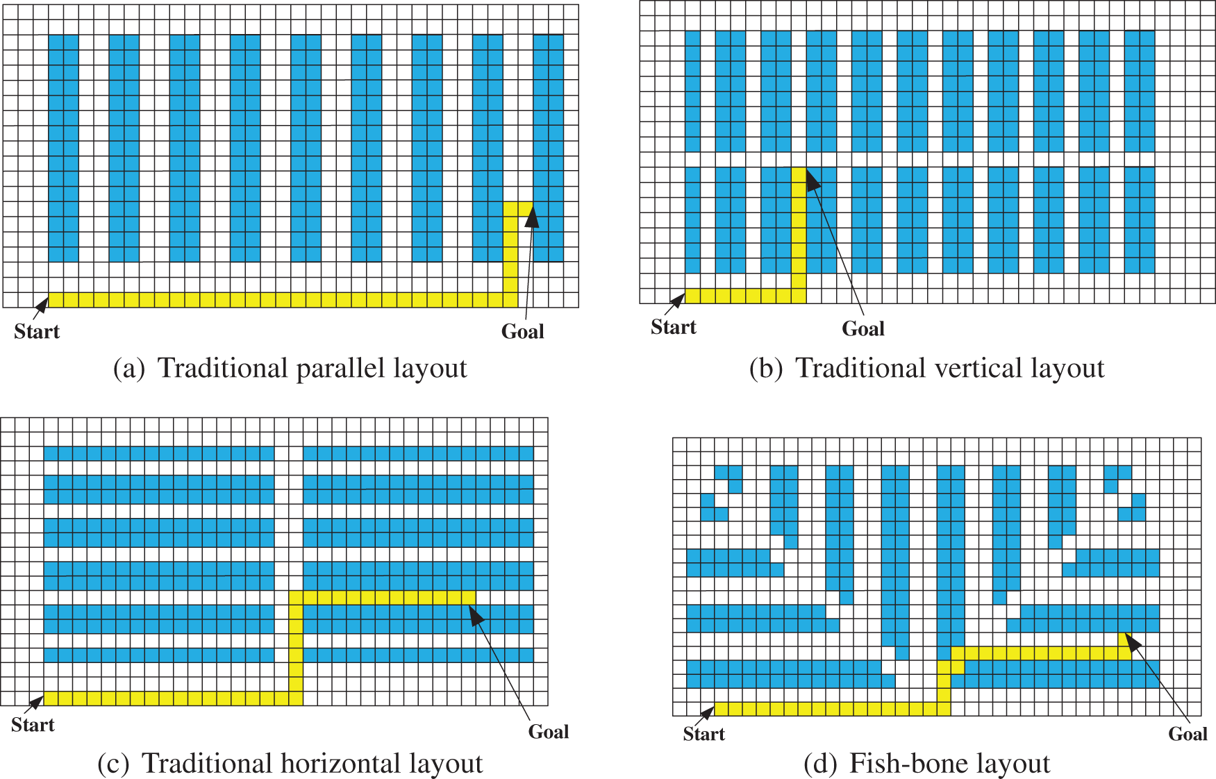
Figure 5: Common warehouse layouts

Figs. 5a–5c are three common environments, where shelves are arranged according to the rules of rows and columns, and there is a channel beside them for accesses; Fig. 5d is a recently developed map due to the rapid development of automated warehouses, and it looks like fish bones. In fish-bone environments, shelves are arranged on both sides of the diagonal. Theoretically, it can increase the storage of goods, but it is inconvenient for AGV access and may lead to a system deadlock because signals may be blocked.

4.1.3 Storage Environments Modeling Methods

The objective of environment modeling is to arrange many workstations and paths in limited areas and present them using mathematics language, and several modeling methods are as follows:

(a) Topological Map Method

The topological map method belongs to graph theory [31], as shown in Fig. 6, where nodes indicate workstations with specific significance, e.g., paths intersections, AGVs parking areas, and AGVs charging locations, etc. The arcs connected between related nodes indicate AGVs’ paths.

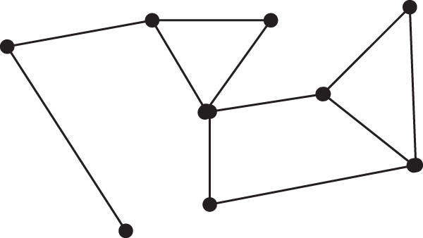
Figure 6: Example of the topological method

A topological map is a high abstraction of natural environments. Instead of measuring the sizes of AGVs or obstacles, we can pay more attention to route-planning strategies.

However, the accuracy is not very satisfying since it neglects the sizes of objects.

(b) Free Space Method

The free-space method operates “bloating” based on the max diameters of obstacles [32]. It considers the obstacles as convex polygons, and divides the environment into obstacles areas (i.e., the grey areas), the obstacles-free regions, and the solid lines indicate AGVs’ paths, as shown in Fig. 7.

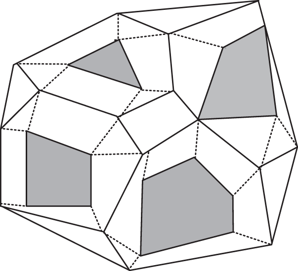
Figure 7: Example of free space method

However, the disadvantage of the method is it may not work well in environments with many obstacles.

(c) Grid Method

The grid method is one of the prevalent environment modeling methods, which has been widely used in mobile robot route planning. The natural environments are abstracted using rasterizing, as shown in Fig. 8. The environment is divided into small grids, and every grid connects others without overlaps [33–35].

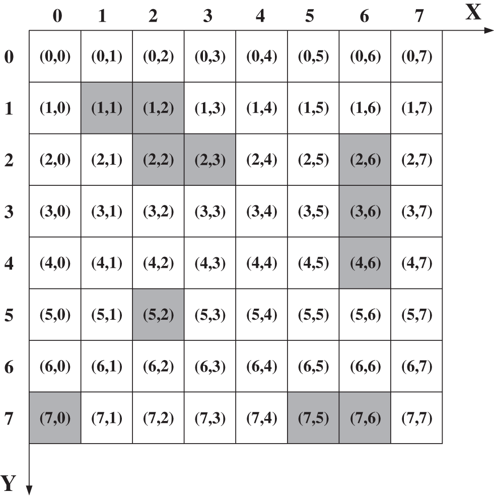
Figure 8: Map of the grid method

The grid map can be classified into the following categories: (a) free grid map, where no obstacles are inside the map; (b) obstacle grid map, where the grid is wholly or partly filled by some obstacles. Every grid denotes a workstation, where the grey grids denote obstacles and the numbers in grids denote the coordinates.

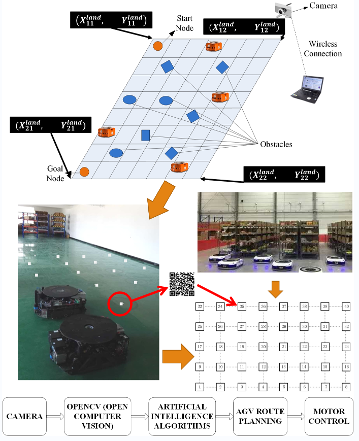
4.1.4 Storage Environments Rasterization and Establishment

In an m×n warehouse, the coordinates of the upper-left corner are (x = 0, y = 0), the lower-right corner is (x = n − 1, y = m − 1), as shown in Fig. 9 [17]. Given the length (or width) of AGVs is LAGV; the length (or width) of each grid is Lgrid=LAGV+δ (δ is a positive number, which indicates the safety margin for AGVs); the length of the storage environment is Lenv and the width is Wenv, so the number of grids in columns is Rgrid=[WenvLgrid] and the number of grids in rows is Cgrid=[LenvLgrid], where [⋅] means down-rounding. Then, the storage environments are divided into n=[Rgrid×Cgrid]′ grids, where [⋅]′ means up-rounding.

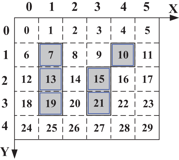
Figure 9: Example of rasterizing storage environments

According to the above rasterizing method, the warehouse environments are designed and planned using OpenCV-Python as follows [36]: (a) taking a picture of the vacant ground and converting it into a standard quadrilateral using Field-Programmable Gate Array (FPGA) [37] and perspective transformation [38,39]; (b) drawing the approximate storage area boundary on the above standard rectangular image, i.e., extracting the storage area using the background filtering and the foreground extraction [40,41]; (c) computing the external enclosing rectangle to obtain the exact area boundary [42]; (d) completing grids division of the storage area, i.e., computing the number of workstations in rows and columns; (e) finishing the environment layout, i.e., reviewing whether the planning results are consistent with the requirements. Since the optimal storage environment layout can be obtained automatically, it significantly reduces the labor force and the energy cost.

4.2 Operation Optimization in Automated Warehouses

4.2.1 Materials Flow in Warehouse

The materials flow consists of the following parts: (a) receiving, i.e., picking up shelves from input locations and transporting them to designated locations; (b) delivering, i.e., picking up shelves from designated locations and transporting them to output locations.

Most of the existing publications conducted shelves-picking decisions sequentially, so the time delay of the previous step may affect the next operations [43]. Xie et al. [44] proposed an integrated shelves-picking procedure by integrating receiving and delivering operations to reduce the influence of delays, and they adopted the conventional task-split following [45] into receiving operations. Moreover, de Koster et al. [26,46] divided the storage area into multiple zones by combining the idea of task-split and zone-control. However, the task splitting may generate additional waiting time because AGVs should visit many stations to collect all parts of the order.

4.2.2 AGVs Fleet Size

Overestimating AGVs fleet size could lead to high cost and frequent congestion, while underestimating may not ensure the completion of tasks [47]. The methods of estimating the optimal AGVs fleet size can be categorized as follows: (a) simulation-based methods; (b) analysis-based methods. To the best of our knowledge, Muller et al. [48] is the first focused on analysis-based methods, he determined the optimal number of AGVs by approximately calculating the total travel time, and they showed that with the increase of the number of AGVs, the average operation time decreases and the average throughput volume increases. Moreover, Ji et al. [49] developed an approximately analysis-based method to estimate the number of AGVs when the total number of idle AGVs is stable. Newton [50] is the first proposed simulation-based method to estimate the minimum of AGVs fleet size, and then Kasilingam et al. [51] developed the model of the method. Although the analysis-based methods may underestimate AGVs’ fleet size compared to simulation-based methods [52], the simulation-based methods are time-required techniques.

4.2.3 Electrical Energy Management

Although the electrical energy management is essential, it is often neglected in publications. A new energy supply way (i.e., Inductive Power Transfer System (IPTS)) is developed currently to replace the traditional way of using batteries, but nearly 8% of the European producers employed IPTS in 2006, and the energy supply using batteries is the most widely used manner [53].

The factors that affect battery management are as follows [54]: (1) the number of charging positions in charging stations; (2) the working time of AGVs before the electric energy level is low. Berenz et al. [55] developed the method of evaluating the risk of battery depletion for AGVs using probability density functions. Kabir et al. [56] developed a method to achieve more running time for AGVs using Targeted State of Charge (TSC), and they showed that the charging time for AGVs could be obtained using optimization, e.g., Petri Net, and applied it in environments such as container terminals and hospitals.

4.2.4 Storage Allocation Policies

(a) Random-Storage Allocation

The random-storage allocation refers to assigning shelves to empty locations with equal probability (e.g., the same travel distance or the same travel time) [57].

However, the policy may lead to low space utilization and increase AGVs travel distances.

(b) Cheapest-Storage Allocation

Herein, the “cheapest” refers to the distance (e.g., Euclidean or Manhattan) being the shortest, or travel time is the least.

The advantages of the policy are as follows [58]: (a) it is easily applied for complex environments; (b) it could perform well if all shelves can be used with the same frequencies. On the other hand, it may lead to imbalance since goods are often stacked around the entrance but emptier gradually towards the back.

(c) Specific-Storage Allocation

It classifies goods into several categories based on their characteristics and stores them in many specific areas, and then it uses a random-storage allocation policy to further choose the storage location in the region [59]. Cruz-DomAnguez et al. [60] employed two-level neural networks in storage allocation, the first level has one neuron, which receives input information and dispatches goods specific channels; the second level has eight neurons, which arrange goods to designated areas.

The objective of the specific-storage allocation is to satisfy the low-storage space requirements, and its advantages are as follows [61]: (a) it can shorten decision-making time if servers are familiar with the layouts; (b) it is suitable for scenarios that goods have different weights and sizes. On the other hand, the space utilization is not high because some locations are reserved only for certain goods.

(d) Full-Turnover-Storage Allocation

The main mechanic of the policy is the Cube-per-Order Rate (COR), i.e., the ratio of total required space and number of AGVs travels.

Therefore, the goods with higher CORs are located at the most accessible locations, and those with lower CORs are located towards the back of the warehouses [54]. Moreover, the turnover rates can change constantly and it may lead to goods overstocks.

(e) Similar-Storage Allocation

The goods allocation belongs to goods clustering problems, which can be solved using median methods. For example, when an AGV needs to pick up two similar goods, it can save more energy if they are closer to each other.

However, most publications fail to notice the possible relationship among goods.

5  Automated Guided Vehicles Scheduling in Warehouses

AGVs can become idle when they finish their current tasks, and the goal nodes of previous tasks are often not the start nodes of the following tasks. Common principles of AGVs scheduling are as follows [62,63]: (a) minimizing AGVs’ travel distances; (b) minimizing AGVs’ waiting time; (c) minimizing number of AGVs; (d) minimizing warehouses’ operation cost.

The scheduling method in warehouses includes: (a) offline AGVs scheduling; (b) online AGVs scheduling, and the methods can be classified into the following categories [64]: (a) First-Come-First-Served (FCFS), which is one of the most widely used methods, and the operation orders entirely depend on the issued time of tasks; (b) greedy method, which is used to minimize operation cost; (c) task priority-based method, the objective of the method is to deliver emergent goods (e.g., fresh foods) to customers as soon as possible.

5.1 Classical AGVs Scheduling Methods

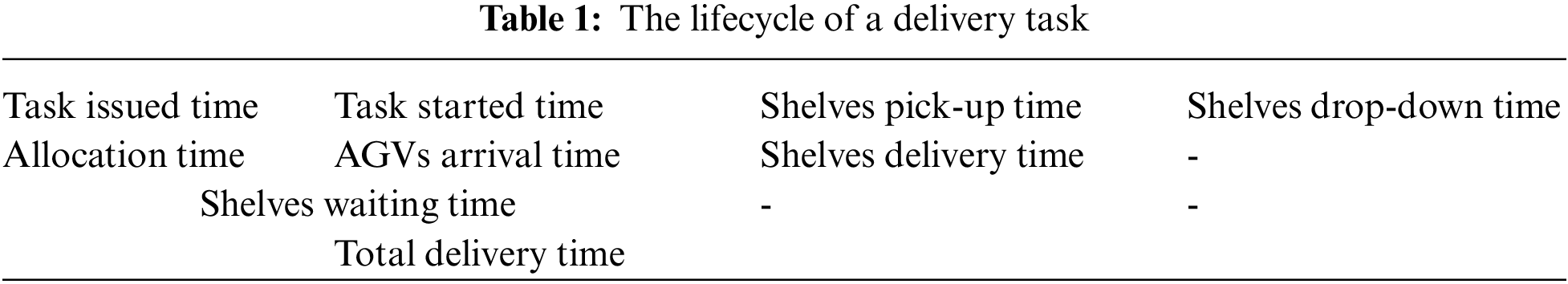
The process of AGVs schedule is as follows [26]: (a) when a task is issued, the start/goal nodes and the expected delivery time are sent to the scheduler at the same time; (b) all possible combinations between AGVs and tasks are generated in scheduler; (c) the distances between AGVs and tasks are computed, an idle AGV with the minimum travel time is selected as the optimal AGV; (d) the computation results are dispatched to the selected AGV. The lifecycle of a delivery task is shown in Table 1.

In general, AGVs scheduling could be categorized as Single-Task Allocation (STA) and Multi-Task Allocation (MTA) [65]: an AGV conducts one task once in STA, which is a commonly used method; MTA refers to assigning multiple tasks to an AGV. However, there are few publications related to MTA even though it can increase the efficiency of systems [66].

Yalcin et al. [67] focused on Puzzle-Based Storage (PBS) scenarios with the minimum number of moves: first, they transformed the problem into a state-space problem; then, they employed the A* algorithm to find an optimal AGV for new issued tasks. Moreover, they presented three estimating functions to estimate the upper bound of escorts’ number in each episode. However, the conventional methods assign tasks only based on the distances between AGV and tasks, which may lead to a local minimum, and traffic congestion may have a significant influence on the performance. Fazlollahtabar et al. [68,69] developed a mathematical model and proposed a heuristic solution by considering the traffic congestions, and they showed that AGVs scheduling and route planning could be combined, but most publications only focused on one of them.

In our opinion, the RL algorithms used in the existing publications can allow AGVs to have learning capabilities (i.e., decide which actions to take at the moment), but the AGVs’ scheduling problem in dynamic or stochastic environments is barely tackled.

5.2 AGVs Scheduling in Chessboard-Like Warehouses

The classical AGVs scheduling methods are not suitable for current environments with many nodes. They failed to notice the problem of energy cost and indicate the characteristics of chessboard-like warehouses, i.e., AGVs can only travel in the cardinal directions and turn at nodes [70].

Most publications used Euclidean distance, i.e., k-Nearest Neighbor (k-NN), to evaluate distance, but the disadvantages of it are as follows: (a) it may not work well when data samples are imbalanced; (b) the computation amount is large for large-scale environments, so it requires data pre-processing; (c) the shortest Euclidean distance does not mean the shortest AGVs traveling distance in grid environments. Therefore, Euclidean distance-based scheduling method is not suitable for chessboard-like warehouses [71].

Manhattan distance represents the sum of the projection lengths of lines between two nodes, i.e., Dm(i,j)=|xi−xj|+|yi−yj|, which indicates the Manhattan distance between Pi(xi,yi) and Pj(xj,yj). Although the computation amount is decreased significantly in grid environments, it does not consider the turns, so the scheduling results may not be the least energy-cost [70]. The Dijkstra’s algorithm is a classical routing algorithm based on graph theory, and we can integrate the AGVs route planning into AGVs scheduling, i.e., the present Dijkstra’s algorithm-based scheduling algorithm. The Dijkstra’s algorithm-based AGVs scheduling algorithm computes the optimal solution using Breadth-First Search (BFS), so that we can obtain not only the location of the optimal agent but also the time-shortest route [72]. Although Dijkstra’s algorithm-based AGVs scheduling algorithm is superior to other algorithms in chessboard-like environments, there are few publications related to chessboard-like warehouses [70] and this research area needs to be further investigated.

6  Automated Guided Vehicles Route Planning in Warehouses

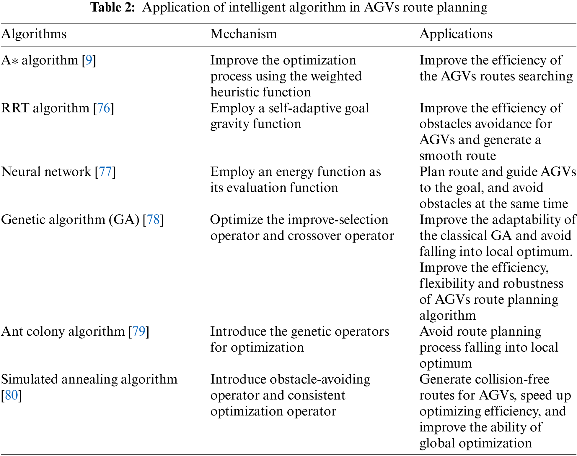
AGVs route planning belongs to the shortest route optimization problem. Common methods include Dijkstra’s algorithm [8], A* algorithm [9], D* algorithm [10,73], Artificial Potential Field (APF) [74], Probabilistic Roadmap (PRM) [75], Rapid Random Tree (RRT) [76], Neural Network [77], Genetic Algorithm [78], Ant Colony Algorithm and other intelligent algorithms [79–81]. Their mechanisms and performs are shown in Table 2. However, management is a challenge because collisions and deadlocks may occur in bidirectional environments, moreover, it is essentially different from the route selection problems of graph theory.

6.1 Single-AGV Route-Planning Methods

6.1.1 Classical Single-AGV Route Planning

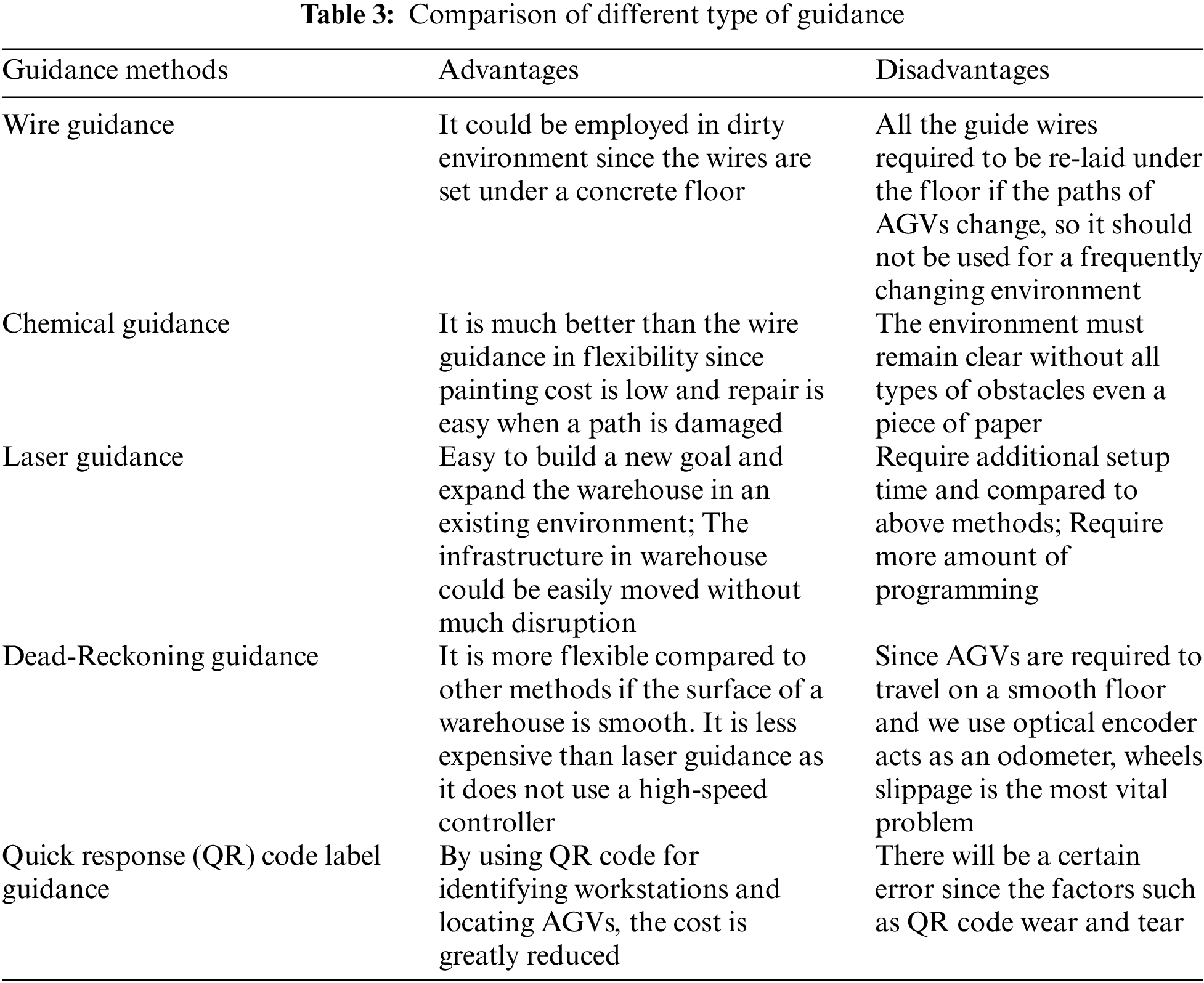
The advantages and disadvantages of several commonly used AGVs guidance systems [82,83] are shown in Table 3.

Single-AGV route planning can be used both in static and dynamic environments, we can use environments perception and local propagation algorithm in static environments, but it is not a trivial task in dynamic environments because the planned routes may be unavailable at some time [84].

Radio-Frequency Identification (RFID) is one of the common route-planning methods, and warehouses could be extended easily using RFID, but the main disadvantage is that accuracy will reduce with the increase of speed under the same weights of shelves [85], as shown in Table 4. Since the sampling frequency is fixed, when AGVs travel faster, the time delay can be more apparent, so we should reduce the speed of AGVs while turning. We can fix a camera at the overhead corner to obtain the locations of AGVs using OpenCV (refer to Section 4), and we can determine their next move using Robot Operating System (ROS), as shown in Fig. 10 [86].

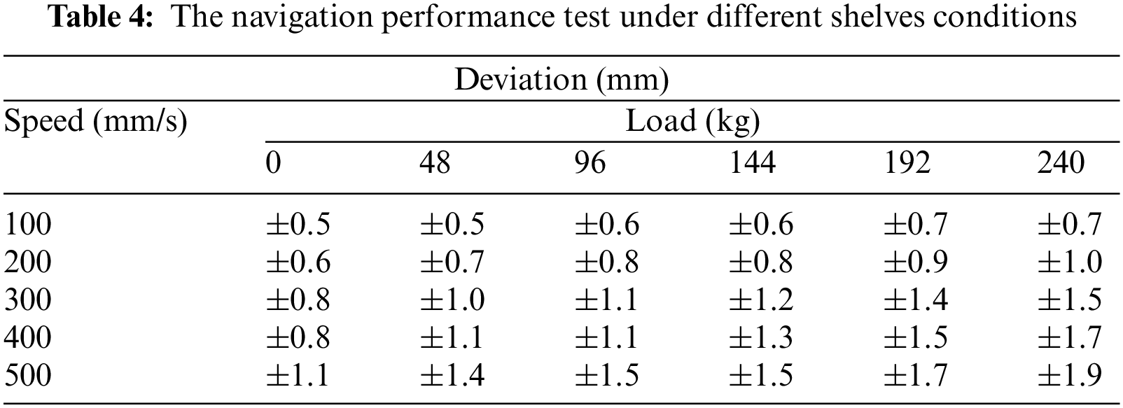
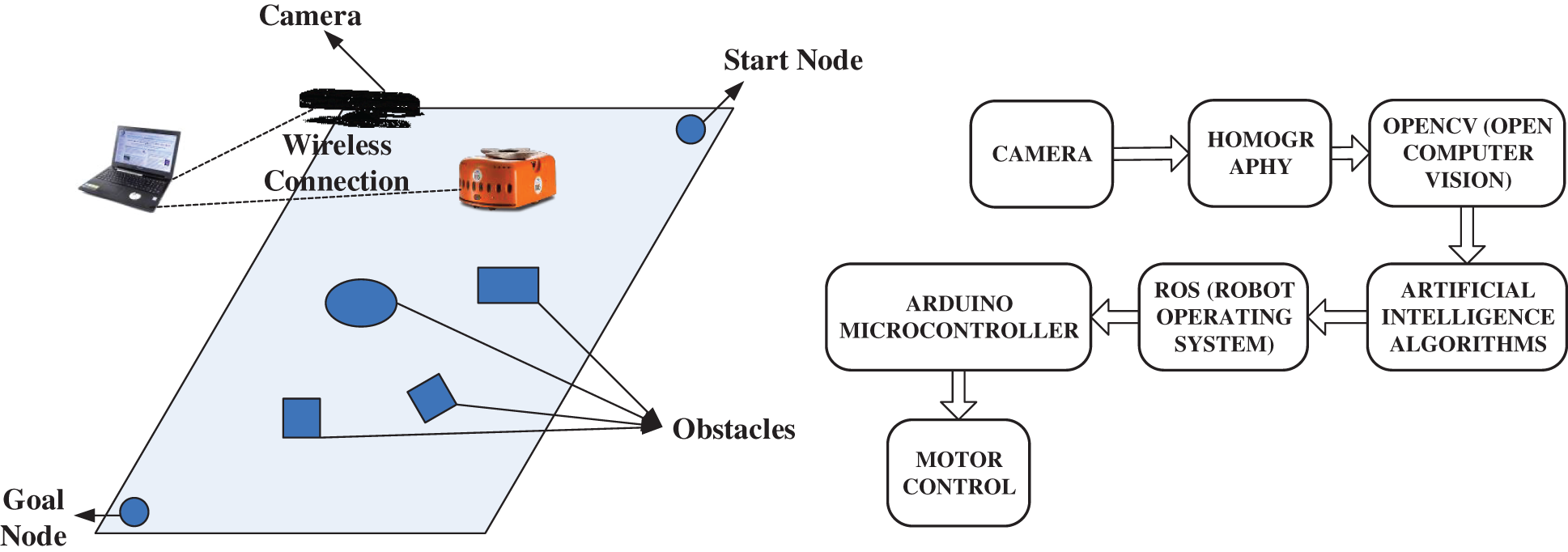
Figure 10: The mechanical design of visual navigation

Since the structure of the Dijkstra’s algorithm is simple, it had been used to perfectly solve the route-planning problem in a small-scale environment [8,72,87–89]. Ogata [90] compared the Dijkstra’s algorithm, the A* algorithm, and the LPA* algorithm (i.e., improved version of the A* algorithm). Since the A* algorithm (or the LPA* algorithm) contains heuristic mechanisms [91], it is more efficient than the Dijkstra’s algorithm in large environments. However, the planned routes may not be optimal sometimes. Moreover, Wu et al. [92,93] presented Colored Resource-Oriented Petri Net (CROPN) models, which can be employed to solve AGVs route-planning problems in environments with a few nodes. Lim et al. [81] divide the free-range environments into many grids to solve the route planning for Unmanned Aerial Vehicles (UAVs).

For simplicity, as shown in Fig. 11, the process of generating equidistant shortest routes from node 1 to node 15 is shown in Table 5.

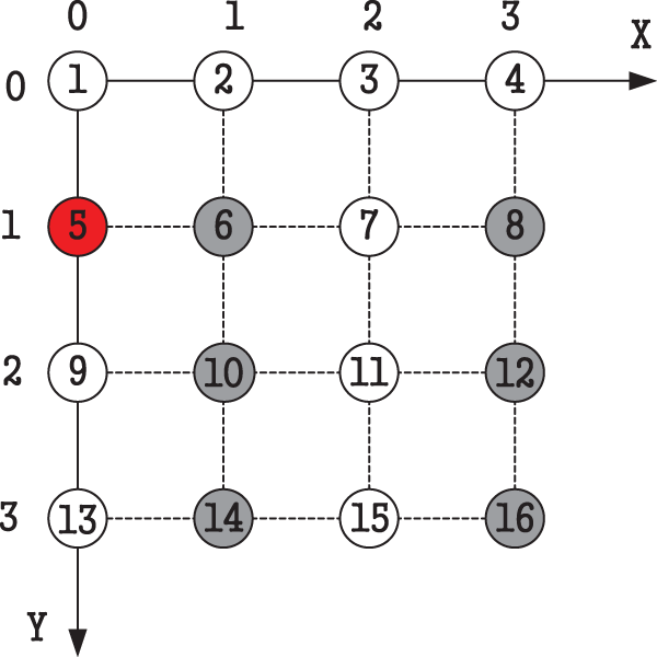
Figure 11: Simplified rasterized warehouse environment

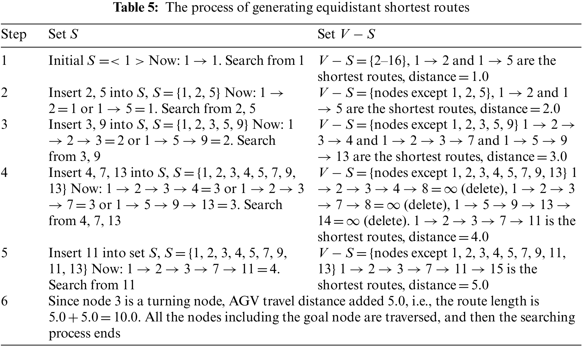
However, the above publications failed to verify the route-planning efficiency of the algorithm in environments with many nodes. The m×n automated warehouses focused in this paper are as shown in Fig. 12a–12c, where m and n represent the number of rows and columns of the environments, respectively. The grey grids indicate obstacles, white grids indicate the channels for AGVs, and numbers in grids indicate the number of nodes (i.e., the number of nodes starting from (x = 0, y = 0) and marked as 1, 2, 3 … n). Red, green, and blue solid squares indicate the start nodes of AGVs, and solid circles indicate their goal nodes [94].

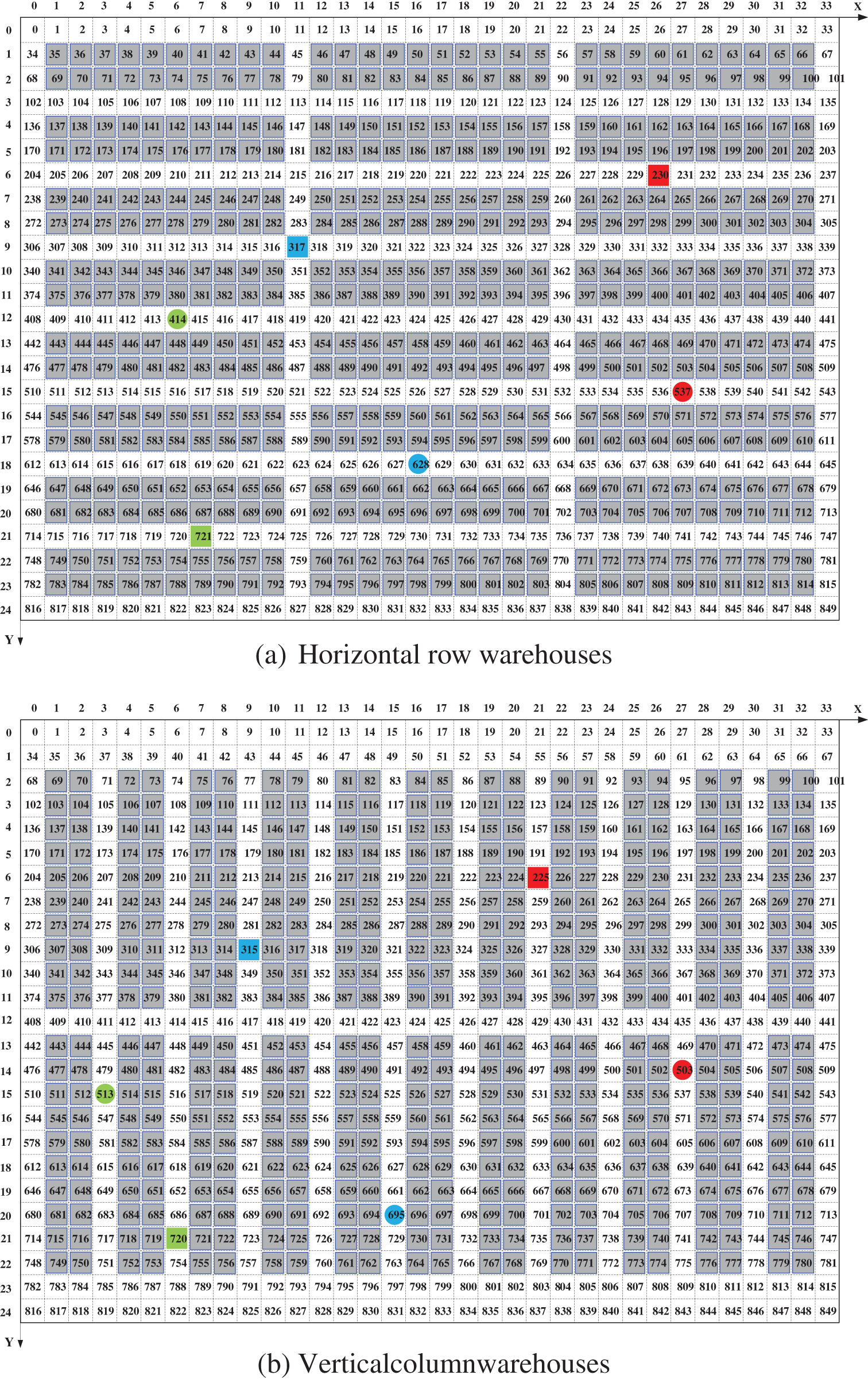
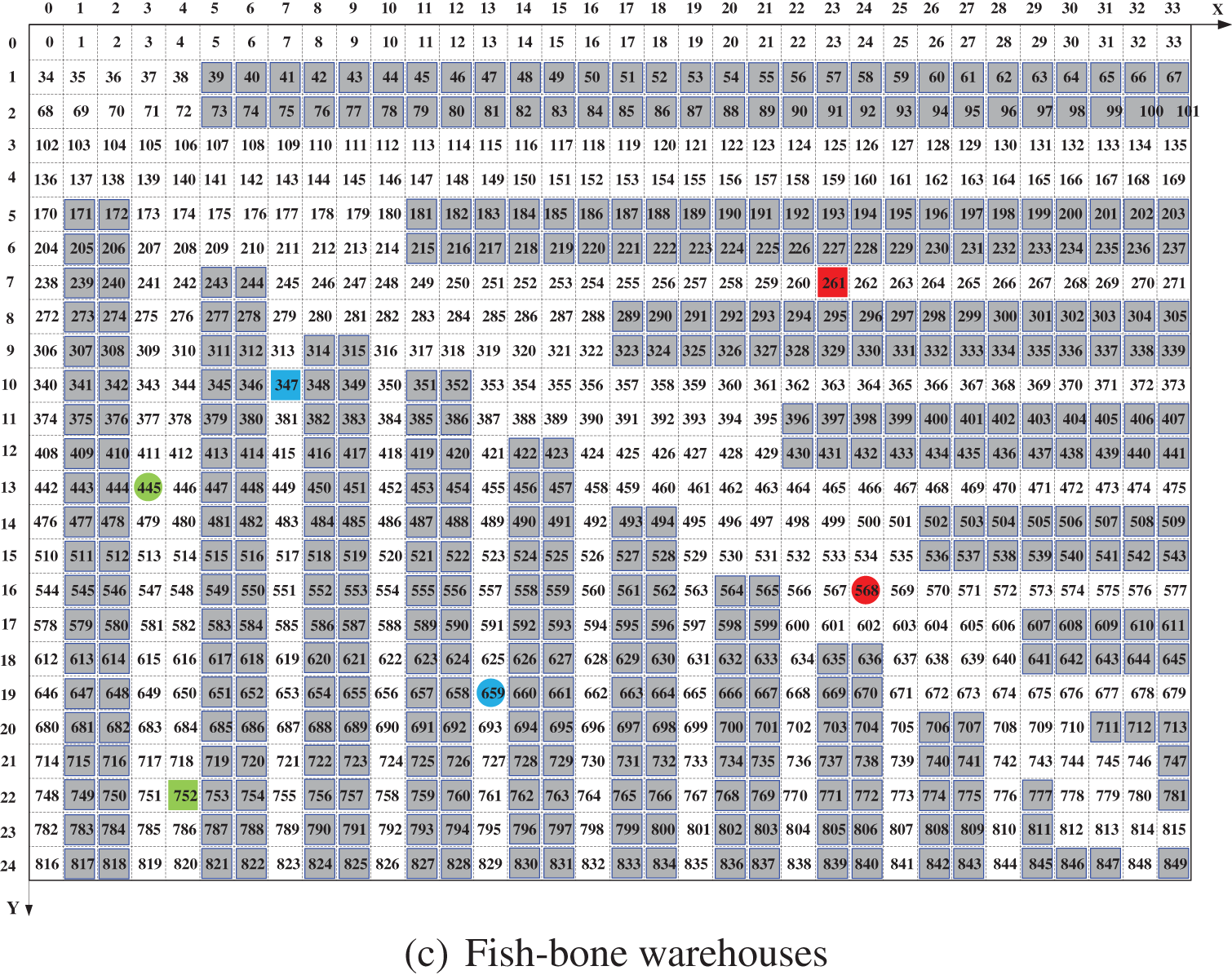
Figure 12: Common paths arrangement patterns

6.1.2 The Shortest Length-Time Dijkstra’s Algorithm-Based Single-AGV Route-Planning Methods

As shown in Fig. 12, the route-planning environments are more complex because more than one equidistant shortest route can exist between two nodes. However, the classical Dijkstra’s algorithm can only find one shortest route and skip over other routes with the same distance.

In our previous work, we improved the classical Dijkstra’s algorithm by considering turns of AGVs to find the optimal routes with both the shortest distance and travel time [72]. The improved Dijkstra’s algorithm reserved all nodes with the same lengths to the source as the intermediate nodes, then searched again from all intermediate nodes until to the goal node. Through multiple iterations, all the shortest routes with the same distance can be found. Moreover, we considered whether a node is a turn or not based on Eq. (1) to reduce the number of turns in the route to improve the efficiency of warehouses.

(Xm+1,Ym+1)−(Xm,Ym)≠(Xm,Ym)−(Xm−1,Ym−1),(1)

where (Xm,Ym) denotes the coordinates of current nodes; (Xm+1,Ym+1) the next nodes; (Xm−1,Ym−1) the previous nodes.

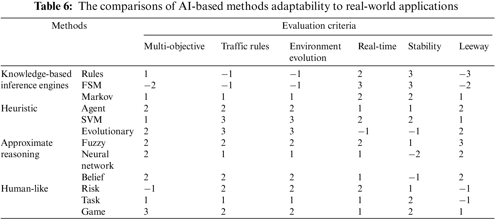
6.1.3 AI-Based Decision-Making Algorithms

The AI-based algorithms are introduced in route planning due to the abilities of thinking, reasoning, and memory, and they can be categorized as follows [95]: (a) knowledge-based algorithm; (b) heuristic algorithm; (c) approximate logic algorithm; (d) cognitive algorithm. The comparisons of the above algorithms in real-world scenarios are shown in Table 6 [96], where the evaluation was indicated with a number scale.

(a) Human-like decision-making algorithms

The learning steps of humans are shown in Table 7 [95].

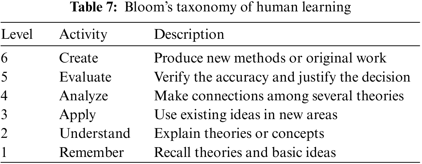
The 1st level is the traditional ability that both humans and computers can have, and no AI is required; the 2nd level refers to extend theories based on current situations; the 3rd level refers to applying AI to test, describe or validate new input data; the 4th level refers to predict, compare and analyze relationships among different elements; the 5th level can be used to make a trade-off in complex systems; the 6th level refers to create new methods, which is the highest level of the human learning.

From our perspective, AI can assist humans for the first three levels and replace humans in the 5th and 6th levels, the successful cases (e.g., parameter setting networks) indicates the possibility of creating.

(b) Heuristic algorithms

The heuristic algorithms were inspired by the natural evolution process, many effective learning methods (e.g., Support Vector Machines (SVM) and Evolutionary Algorithm (EA)) can be employed, and the most common heuristic algorithm for AGVs route planning is the A* algorithm [97].

The advantages of heuristic algorithms are as follows: (a) reducing computation complexity in small environments; (b) running faster than exhaustive methods. However, it uses the current state rather than the global state, so that it could lead to a locally optimal solution.

(c) Approximate reasoning algorithms

The approximate reasoning algorithms contained multi-valued logic, so the solutions have approximation dimensions. Recently, Artificial Neurons Networks (ANNs) have contributed an alternative method for approximating, and the approximate reasoning algorithm is close to the human reasoning process.

The advantage of approximate reasoning algorithms is they are fuzzy-based methods, so the demand for accuracy is not strict. On the other hand, the challenging problem is to ensure learning correctly [98], so some labeled data is needed to increase the accuracy.

(d) Knowledge-based inference engines

The knowledge-based inference engines rely on deductive reasoning mechanisms, and the most popular algorithm is the rules-based reasoning algorithm (e.g., Expert System (ES)) [99]. Another common model is Finite State Machine (FSM), i.e., the systems are described using several states and transitions among them, and both the ES and the FSM are triggered by environmental changes. Moreover, warehouses could be extended to dynamic Bayesian networks with Markov properties [100,101].

The advantage of knowledge-based inference engines is they are robust in any unexpected situations. On the other hand, they are prior knowledge required methods.

6.1.4 AI-based Single-AGV Route-Planning Algorithms

(a) Artificial Neural Networks

Due to the merit of nonlinear functional approximation, Artificial Neural Networks (ANNs) [102,103] are commonly used in route planning [104], and the process is as follows: (a) choosing the maximum incentive from receiving domain like the main input stimulus; (b) choosing a neuron with the maximum incentive as the next neuron if there is a path to the target neuron; (c) repeating above steps, the routes from the start nodes to the goal nodes are obtained.

The common ANNs are as follows [105,106]: (a) multi-layer Forward Networks, which can be used in any unknown environments [107]; (b) Hopfield Neural Networks (HNNs) [108]; (c) Fuzzy Neural Networks (FNNs); (d) Radial Basis Function Neural Networks (RBFNNs); (e) Adaptive Resonance Theory Neural Networks (ARTNNs) [109], which belong to competitive neural networks. Since ARTNNs do not forget the old knowledge while learning new knowledge, they can avoid local minimum; (f) Self-Organizing Map Neural Networks (SOMNNs) [110], which also belong to competitive neural networks. Since the optimization process can run automatically, they have some similarities with the human brain;

The advantages of ANNs are as follows [111]: (a) they have strong robustness and fault tolerance, and information is stored in distributed ways; (b) they are easy for parallel processing; (c) they can be employed in uncertain systems because they can approximate any nonlinear function; (d) they have strong ability of information processing, and they can deal with both quantitative and qualitative problems. On the other hand, the convergence time of ANNs is long for large-scale environments, so there are no applications in real-world warehouses.

(b) Markov Decision Process

Markov Decision Process (MDP) is a fundamental theory of Reinforcement Learning (RL) [112–115]. MDP can be described as a quintuple (i.e., ⟨S,A,P,R,γ⟩), where S indicates the finite states set, A the actions set, and P the state transition probability matrix [116]. Based on the outputs of P and R, MDP can be classified as deterministic MDP and stochastic MDP, where the outputs are fixed in deterministic MDP, but they are certain distributions in stochastic MDP. Given the probability for entering any adjacent node of AGVs in m×n warehouses are Pij, where i indicates the current state of the AGV (i.e., St), j indicates its next state (i.e., St+1), and P matrix can be described as follows [17]:

P=[P11P12P13…P1nP21P22P23…P2nP31P32P33…P3n……………Pm1Pm2Pm3…Pmn].(2)

The objective of the MDP method is to find a policy to minimize cost function (e.g., time or energy) and maximize positive function (e.g., routes reward or efficiency).

(c) Q-Learning Algorithm

(i) The Classical Q-Learning Algorithm

The supervised learning algorithms are commonly used in route planning, but they are often non-robust to even small environmental changes [117]. The Q-learning algorithm belongs to model-free RL [118–120], which can be considered as asynchronous Dynamic Programming. The Q-learning algorithm relies on rewards and punishments, rather than prior training instances. The learning process of the Q-learning is similar to the classical Temporal Differences (TD) [121], i.e., agents choose proper actions as the next moves to maximize accumulated rewards [122–124]. The pseudo-code of the Q-learning algorithm [125,126] is shown in Algorithm 1.

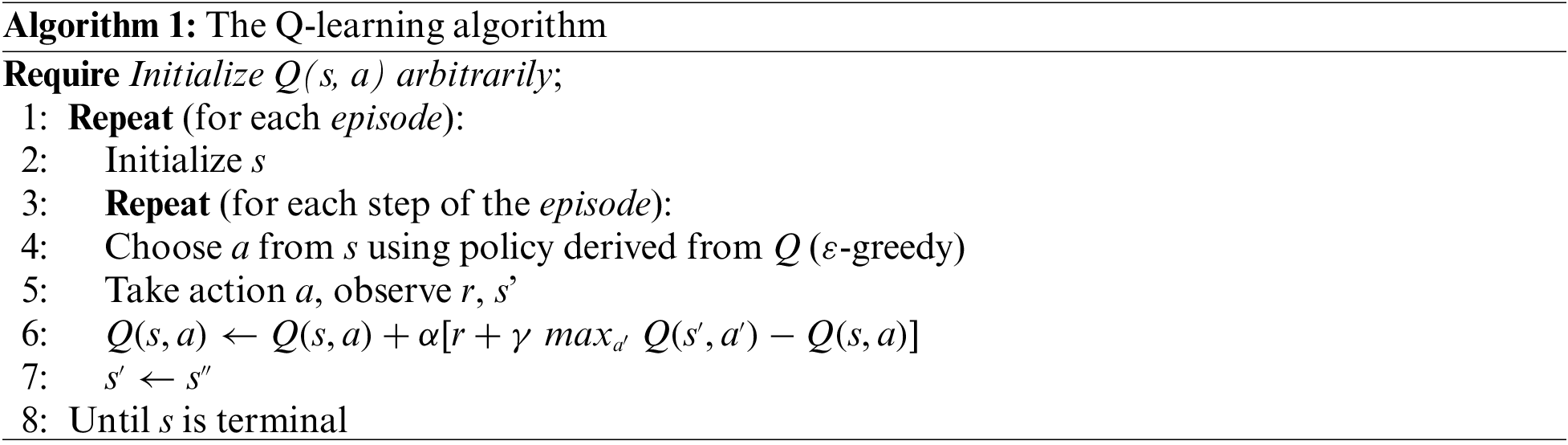
The advantages of the Q-learning-based route-planning algorithm are as follows [127]: (a) it can deal with route-planning problems in any dimension; (b) it is a model-free algorithm, and it can be used to find optimal actions with any given MDPs. On the other hand, it requires large computations for convergence and large storage to save all the possible actions [128].

(ii) Some varieties of Q-Learning Algorithm

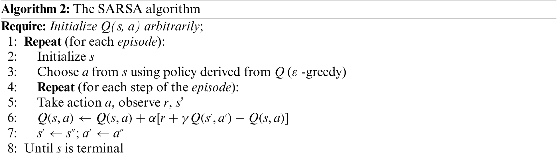
SARSA (State-Action-Reward-State-Action) algorithm uses the form of Q-table and chooses actions with the larger Q-value in the environment as well, as shown in Algorithm 2. But there are some differences between the Q-learning algorithm and the SARSA algorithm, for one thing, the Q-learning algorithm is an off-policy algorithm, but the SARSA algorithm is an on-policy algorithm; for another, the Q-learning algorithm uses Bellman Equation with max Q to update Q(s, a), but the SARSA algorithm updates Q(s, a) using Bellman Equation without max Q. Therefore, the Q-learning algorithm will always choose the shortest route to the goal no matter how dangerous it is, but the SARSA algorithm is quite conservative [129].

Aleo et al. [130] focused on constrained route-planning problems with end-effect, and they introduced the SARSA algorithm in robot route-planning areas. Although the SARSA algorithm can converge to the optimal solution with finite state space, its efficiency has become a vital issue regarding further development. SARSA (λ) is an improved version of the SARSA algorithm, and it improved the convergence using Eligibility Trace (i.e., backward propagation). Fu et al. [131] developed a fast SARSA (λ) algorithm based on 2nd order TD error (i.e., SOE-SARSA (λ)) to improve the convergence rate.

Moreover, Adaptive Heuristic Critic (AHC) algorithm is another alternative method, which used critic-learning mechanisms, and Gachet et al. [132] were the first to employ the AHC algorithm in mobile robot control, they used it to determine proper actions.

From our perspective, it can provide AGVs with the ability to choose optimal actions (i.e., going forward, turning left, turning right, or stopping) by combining the AHC algorithm and the TD algorithm.

(d) ANNs Combined with Q-learning algorithm

Since the learning speed is low only using the ANNs, and it is impossible to learn all the states only using the Q-learning algorithm, we can combine them to overcome the disadvantages of either [133]. In general, there are five outputs for AGVs in warehouses, i.e., travel forward, stop, turn left 90°, turn right 90° and self-rotate 180° [13], Demircan et al. [134] used ANNs to create route-planning controllers and then used Q-learning algorithm to collect training data for ANNs. Zalama et al. [135] developed a control strategy to choose actions, the Q-learning algorithm is used to determine the behavior and compute the travel velocity of AGVs, and ANNs are used to improve learning operation.

Deep Q-Networks (DQN) is generated by combining the ANNs and the Q-learning algorithms. The preliminary studies of employing the DQN in AGVs route planning on square grids world, showed that the DQN can perform robustly on square grids world [133,136,137].

(e) Reducing Iteration Time of Q-Learning Algorithm

Smart automated warehouses are real-time requirement systems, AGVs should respond to tasks as soon as possible, so we need to pay more attention to computing time. No matter Q-learning algorithm, AHC algorithm, or other RL algorithms, they are operated based on Q-table, i.e., learning from behaviors of agents through trial-and-error to build the optimal Q-table. We can learn from graph theory to decrease the Q-table convergence time.

Since there are many obstacles (i.e., negative rewards) in warehouses, the iteration for the classical Q-learning algorithm is very time-consuming. On the other hand, the Dijkstra’s algorithm uses an adjacency matrix to describe environments, so it runs faster than the Q-learning algorithm in the presence of obstacles. Inspired by this observation, we can develop a novel method by integrating the Dijkstra’s algorithm and the Q-learning algorithm to reduce the iteration time and improve the efficiency of systems: First, we could combine the adjacency matrix of the Dijkstra’s algorithm and reward matrix of the Q-learning algorithm into a new matrix (i.e., Adjacency-Reward (A-R)), and use it to describe environments. Moreover, before AGVs travel, we need to iterate the A-R matrix multiple times to obtain the optimal Q-table, and the dimension of the reward matrix and adjacency matrix are both n2×n2 for n×n environments and it takes a long time for iterating. We propose a low-dimensional A-R matrix to describe the environment by considering AGVs’ start (and goal) nodes.

(f) Dynamic Programming and Monte-Carlo Search Tree Algorithms

(i) Dynamic Programming-Based Route-Planning Algorithm

The computation of value function is a recursive process, and we need to evaluate the rewards of all adjacent states based on the current state, and the state with the largest reward is taken as AGV’s next state. As shown in Fig. 12, the method of computing relationship between the current node and all adjacent nodes is [17]:

VT+1(s)=∑s+1p(st+1|st,at)[ratst+1+γVst+1T],(3)

where p(st+1|st,at) indicates the probability of transferring to adjacent state st+1 based on the current state st by taking action at; ratst+1 indicates the reward of transferring to state st+1 by taking action at; γ the discount factor, γ∈[0,1]; VT(st+1) the value of each state adjacent to state st.

Without considering obstacle nodes in warehouses, the probability is the same for traveling to surrounding nodes, i.e., p(st+1|st,at)=14, γ=1. Eq. (3) can be rewritten as [94]:

VT+1=14×[(−1+1×VuT)+(−1+1×VdT)+(−1+1×VlT)+(−1+1×VrT),(4)

where VuT, VdT, VlT,VrT denote the state value of upper, lower, left, and right adjacent nodes of AGV’s current nodes, respectively.

(ii) Route-Planning Method of Combining Dynamic Programming and Monte-Carlo Search Tree

The Monte-Carlo Search Tree algorithm can be combined with the Dynamic Programming to improve the speed of route planning [94]. First, the classical Monte-Carlo Search Tree algorithm is improved by following steps: (1) the “cutting” operations is added into the “searching” process to determine the expanding directions of search trees; (2) the single-step update is employed for establishing search trees to move the “back-propagation” process ahead of the “simulation” process; (3) the evaluation criteria based on “Move value” is proposed to find the time shortest routes.

Then, the idea of the multi-stage optimization of the Dynamic Programming is introduced, the warehouses are divided based on AGVs’ start nodes and their goal nodes. The objective is to increase the efficiency of route planning by reducing the range of route searching.

6.2 Multi-AGV Collision-Free Route-Planning Methods

6.2.1 Classical Multi-AGV Route-Planning Methods

Multi-AGV collision-free route planning belongs to the Multi-Agent Path-Finding (MAPF) problem [138–141], and the most popular methods are time window-based methods [21]. There was an improved Dijkstra’s algorithm-based multi-AGV self-adaptive collision-free route-planning approach as follows [87]: it planned routes for each task based on the improved Dijkstra’s algorithm [72]; then, it detected and classified potential collisions upon the comparison of nodes’ coordinates and occupancy time; finally, a self-adaptive strategy is proposed to solve the potential collisions according to the collisions’ types. It presented three strategies as follows: (a) one of the AGVs waits for 5 s or slows down before entering the node; (b) the computer modifies the route of one of AGVs; (c) the system reissues the tasks.

Another common multi-AGV route-planning method is zone-based strategy, i.e., dividing the route-planning area into many non-overlapping zones and only one AGV in a zone at a time. The traditional zone-based strategy belongs to fixed strategies, where AGVs are not allowed to access other areas, but it can’t work well if the loads are imbalanced among different zones. Ho et al. [20] developed a dynamic zone-based strategy, which improved the traditional strategy in the following aspects: (a) it used zone partition design to maintain balance among different zones, where the zone partition was determined by a relationship coefficient; (b) it improved the traditional design using Simulated Annealing.

The multi-AGV systems are timed discrete event systems and Colored Timed Petri Net (CTPN) is an effective method for modeling, Wu et al. [93] developed a deadlock-free modeling method based on CTPN, and they integrated it with colored edges to build digraphs of routes. However, most publications considered route-planning problems as static problems [142,143], they built time windows for dynamic obstacles and then used local route-planning methods to solve collision-free problems. Despite the effectiveness, it may lead to a sub-optimal solution. Phillips et al. [144] developed an algorithm based on contiguous safe intervals, and the process is as follows: (a) graph construction, i.e., creating timelines for every spatial configuration using predicted obstacle trajectories; (b) graph search, i.e., operating route planning using A* algorithm. However, the proposed method does not work well in larger environments. However, the proposed method does not work well in larger environments.

Yan et al. [145] presented two types of travel patterns for AGVs to simplify route planning: (a) cross model; (b) local loop model. As shown in Fig. 13, the shaded grids represent the locations of shelves and other grids represent channels, the grids marked with dots represent intersections, and the arrows indicate directions of channels.

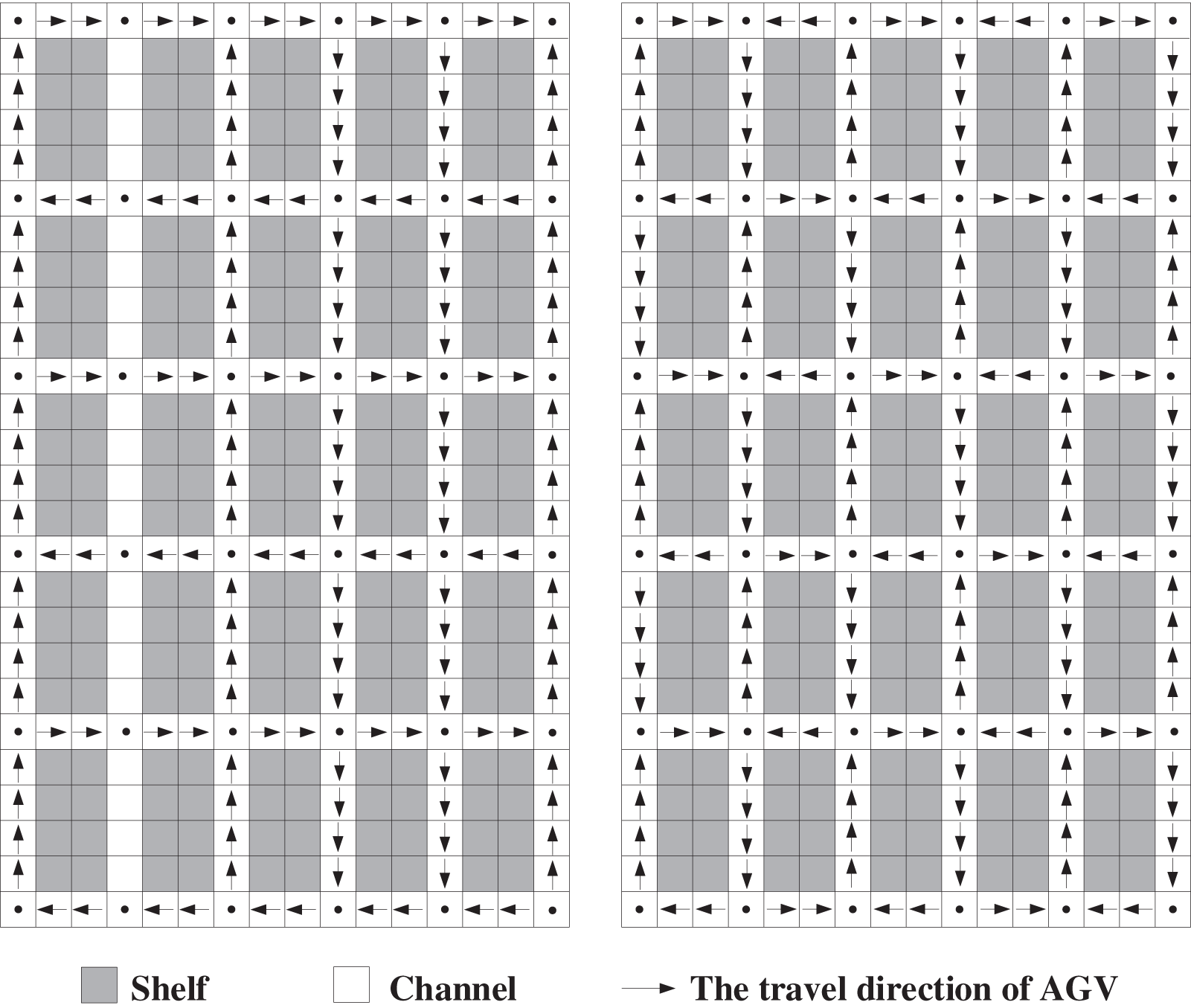
Figure 13: AGVs travel direction patterns

If there are two AGVs in a collision, the most straightforward routes re-planned method is to delete one of AGV’s routes and plan the sub-optimal shortest route for it [146], but it may be difficult for route planning using if-then rules when the number of AGVs becomes large. We can employ the human mind, more specifically, Artificial Intelligence (AI), in route planning to develop the ability of learning.

6.2.2 AI-Based Multi-AGV Route-Planning Algorithms

The state-of-the-art multi-AGV route planning algorithms considered every AGV as an individual with the ability to act autonomously, i.e., AGVs are equipped with sensors to measure distances to others and detect their positions [147].

Recent work in RL and Deep Reinforcement Learning (DRL) have shown their effectiveness in multi-AGV decision-making problems. Zhang et al. [148] employed the Q-learning algorithm to solve the multi-AGV route-planning problem in urban roads networks scenarios, and they presented that the optimal route may not always be available if an unknown emergency occurs. Panov et al. [133] proposed a multi-AGV fleet coordination algorithm in smart city environments, they combined Convolutional Neural Networks (CNNs) and DRL to make AGVs fulfill tasks in large environments, and they employed the Transfer Learning (TL) to balance multiple objectives. We noticed the paper because the urban scenarios are similar to warehouses.

Similar to single-AGV AI-based route planning, there is also the problem of the “curse of dimensionality” and it needs to reduce state space for route planning. For example, Burkov et al. [149] used the Adaptive Play Q-Learning (APQ) algorithm [150] to restrict the searching space for multi-AGV route planning.

6.2.3 Collisions Resolution Policies Based on Conflicts Classifications

When environments become larger, the number of AGVs and collisions may increase significantly. Despite its effectiveness, the self-adaptive multi-AGV collisions resolution may increase the computation burden of warehouses [87]. Therefore, a collision classification-based approach is proposed to improve the real-time performance of systems [88]: First, the collisions in warehouses can be classified into four classifications, as shown in Fig. 14.

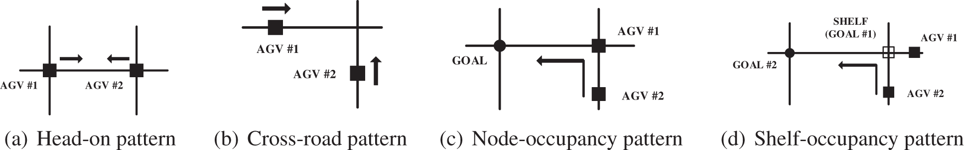
Figure 14: Common collision classifications

Second, the collision in Fig. 14d can be further classified into two types based on whether AGVs are loaded or not. Third, four feasible solutions for the above collisions classifications are presented as follows: (a) selecting the alternative route; (b) waiting for a period before starting to reduce the energy cost of multiple starts and stops; (c) modifying the planned routes; (d) re-dispatching tasks. Fourth, the corresponding solution for each collision classification is selected based on experiments and analyses results. It is worth mentioning that solution (a) and (c) is suitable for collision classification of Fig. 14a; solution (b) is suitable for Fig. 14b; solution (a) and (c) are both suitable for Fig. 14c.

6.2.4 Collisions Resolution Policies Based on Critical Sections

The critical section refers to the parts that contain repeated nodes. This section discusses the location of the collision, and AGVs cannot be regarded as nodes because AGVs should have safety distances to others.

The function of critical sections is to reduce the time wasted finding exact locations of collisions. Manhattan distance indicates the sum of the projection distances of lines formed by two nodes, for example, the Manhattan distance between node Pi(xi,yi) and node Pj(xj,yj) is dm(Pi,Pj)=|xi−xj|+|yi−yj|. The AGV with a smaller Manhattan distance is considered to be modified to minimize the total time of systems, and resolution is as follows [70]: (i) if the goal node of the AGV with a bigger Manhattan distance (i.e., AGV1) is on the route of the AGV with smaller Manhattan distance (i.e., AGV2), AGV2 should wait for Len×tc+tw (s) before entering the critical sections; (ii) if not, it should wait for Len×tc (s).

The advantages of the critical section-based method compared to the time window-based method [21] are as follows: (1) improves system robustness: it ensures that only one AGV in a certain section avoids collision and ensures the safety margin for AGVs driving; (2) improves the conflict detection efficiency: the coordinates of each of the two nodes and the time of AGVs passing through this node are compared in time window-based method. Although the detection accuracy is improved, the detection efficiency is reduced. In this method, the routes of AGVs are compared in pairs, and if the repeated nodes exist, the length of the critical sections is calculated, otherwise, exiting, so the numbers of comparisons are significantly reduced; (3) reduces computing complexity: it omits the division of conflict types, which improves algorithm’s robustness, reduces the difficulty in applicability, and increases practicability.

7  Conclusion

This paper presented a comprehensive survey on the application of AGVs in warehouses while discussing some key issues, i.e., AGVs systems, warehouse layout, operation optimization, AGVs scheduling, AGVs routing problem, and AI applications in warehouses. Both centralized and decentralized AGVs systems have their advantages and disadvantages. The warehouse layout and operation optimization (including AGV electrical energy management) play significant roles in building flexible logistic systems. Moreover, AGVs scheduling and route planning are essential for minimizing tasks operation time in current chessboard-like environments. By employing the AI (e.g., RL algorithms), we can avoid the effectiveness of route-planning algorithms being afflicted by any minor environmental changes. However, the efficiency of RL algorithms can be reduced with the increasing environmental scales. Thus, we proposed an original novel method to accelerate the route-planning efficiency by combining the RL algorithms and Dijkstra’s algorithm.

After reviewing key publications on applications of AGVs in warehouses, we found some problems needed to be further concerned as follows:

•   Although the problem of AGVs scheduling has been researched for a long time, the dynamic scheduling methods in chessboard-like warehouses are not adequately attended and discussed. Moreover, integrating idle AGV parking factors into scheduling problems is necessary.

•   With the increase of environmental scales, AGVs route planning becomes more complex because the number of nodes is large and routes with the shortest distance may not be the most energy-saving routes. Although the classical AI-based route-planning algorithms (e.g., the Q-learning algorithm) work well in AGV route planning, they have some limitations (e.g., the convergence time is large). However, very few publications fundamentally reduce the training time. Therefore, it is an important part of our future work.

•   Smart automated warehouses have become more popular. Also, AGVs should be capable of self-learning and self-adaption. Therefore, the flexibility of dealing with environmental changes is more important and few studies have been conducted in this research direction. It is another important part of our future work.

Funding Statement: The authors received no specific funding for this study.

Conflicts of Interest: The authors declare that they have no conflicts of interest to report regarding the present study.

References

 1.  Kvasnica, I., Kvasnica, P. (2015). Accuracy of mathematical models in simulator distributed computing. Computer Modeling in Engineering & Sciences, 107(6), 447–462. DOI 10.3970/cmes.2015.107.447. [Google Scholar] [CrossRef]

 2.  Serrato-Garcia, M. A., Mora-Vargas, J., Murillo, R. T. (2016). Multi objective optimization for humanitarian logistics operations through the use of mobile technologies. Journal of Humanitarian Logistics and Supply Chain Management, 6(3), 399–418. DOI 10.1108/JHLSCM-01-2015-0002. [Google Scholar] [CrossRef]

 3.  Vengerov, D. (2009). A reinforcement learning framework for utility-based scheduling in resource-constrained systems. Future Generation Computer Systems, 25(7), 728–736. DOI 10.1016/j.future.2008.02.006. [Google Scholar] [CrossRef]

 4.  Poullet, J., Parmentier, A. (2020). Shift planning under delay uncertainty at air France: A vehicle-scheduling problem with outsourcing. Transportation Science, 54(4), 956–972. DOI 10.1287/trsc.2019.0960. [Google Scholar] [CrossRef]

 5.  Oh, B. H., Kim, K., Choi, H. L., Hwang, I. (2018). Cooperative multiple agent-based algorithm for evacuation planning for victims with different urgencies. Journal of Aerospace Information Systems, 15(6), 382–395. DOI 10.2514/1.I010589. [Google Scholar] [CrossRef]

 6.  Koeln, J. P., Alleyne, A. G. (2018). Robust hierarchical model predictive control of graph-based power flow systems. Automatica, 96, 127–133. DOI 10.1016/j.automatica.2018.06.042. [Google Scholar] [CrossRef]

 7.  Jiang, B., Bishop, A. N., Anderson, B. D., Drake, S. P. (2015). Optimal path planning and sensor placement for mobile target detection. Automatica, 60, 127–139. DOI 10.1016/j.automatica.2015.07.007. [Google Scholar] [CrossRef]

 8.  Dijkstra, E. W. (1959). A note on two problems in connexion with graphs. Numerische Mathematik, 1, 269–271. DOI 10.1007/BF01386390. [Google Scholar] [CrossRef]

 9.  Pal, A., Tiwari, R., Shukla, A. (2012). Modified A* algorithm for mobile robot path planning. In: Soft computing techniques in vision science. Germany: Springer. [Google Scholar]

10. Jiang, L., Wang, S., Meng, J., Zhang, X., Xie, Y. (2019). A fast path planning method for mobile robot based on voronoi diagram and improved D* algorithm. 2019 IEEE/ASME International Conference on Advanced Intelligent Mechatronics (AIM), Hong Kong, China. [Google Scholar]

11. Xu, Z., Guo, S., Song, T., Li, Y., Zeng, L. (2022). Localization of mobile robot aided for large-scale construction based on optimized artificial landmark map in ongoing scene. Computer Modeling in Engineering & Sciences, 130(3), 1853–1882. DOI 10.32604/cmes.2022.018004. [Google Scholar] [CrossRef]

12. Wang, F. Y., Zhang, J. J., Zheng, X., Wang, X., Yuan, Y. et al. (2016). Where does alphago go: From church-turing thesis to alphago thesis and beyond. IEEE/CAA Journal of Automatica Sinica, 3(2), 113–120. DOI 10.1109/JAS.2016.7471613. [Google Scholar] [CrossRef]

13. Dubey, A., Mishra, R., Jha, A. (2013). Path planning of mobile robot using reinforcement based artificial neural network. International Journal of Advances in Engineering & Technology, 6(2), 780–788. [Google Scholar]

14. Hang, M., Koenig, S., Ayanian, N., Cohen, L., Sharon, G. (2016). Overview: Generalizations of multi-agent path finding to real-world scenarios. IJCAI-16 Workshop on Multi-Agent Path Finding, New York, USA. [Google Scholar]

15. Barenji, A. V., Barenji, R. V., Roudi, D., Hashemipour, M. (2017). A dynamic multi-agent-based scheduling approach for smes. The International Journal of Advanced Manufacturing Technology, 89(9–12), 3123–3137. DOI 10.1007/s00170-016-9299-4. [Google Scholar] [CrossRef]

16. Yu, J., LaValle, S. M. (2013). Multi-agent path planning and network flow. In: Algorithmic foundations of robotics X, pp. 157–173. Germany: Springer. [Google Scholar]

17. Cardarelli, E., Digani, V., Sabattini, L., Secchi, C., Fantuzzi, C. (2017). Cooperative cloud robotics architecture for the coordination of multi-AGV systems in industrial warehouses. Mechatronics, 45, 1–13. DOI 10.1016/j.mechatronics.2017.04.005. [Google Scholar] [CrossRef]

18. Olmi, R., Secchi, C., Fantuzzi, C. (2011). An efficient control strategy for the traffic coordination of AGVs. 2011 IEEE/RSJ International Conference on Intelligent Robots and Systems, Japan, IEEE. [Google Scholar]

19. Secchi, C., Olmi, R., Fantuzzi, C., Casarini, M. (2014). Trafcon–Traffic control of AGVS in automatic warehouses. In: Gearing up and accelerating cross-fertilization between academic and industrial robotics research in europe, pp. 85–105. Germany: Springer. [Google Scholar]

20. Ho, Y. C., Liao, T. W. (2009). Zone design and control for vehicle collision prevention and load balancing in a zone control AGV system. Computers & Industrial Engineering, 56(1), 417–432. DOI 10.1016/j.cie.2008.07.007. [Google Scholar] [CrossRef]

21. Smolic-Rocak, N., Bogdan, S., Kovacic, Z., Petrovic, T. (2009). Time windows based dynamic routing in multi-AGV systems. IEEE Transactions on Automation Science and Engineering, 7(1), 151–155. DOI 10.1109/TASE.2009.2016350. [Google Scholar] [CrossRef]

22. Draganjac, I., Miklic, D., Kovacic, Z., Vasiljevic, G., Bogdan, S. (2016). Decentralized control of multi-AGV systems in autonomous warehousing applications. IEEE Transactions on Automation Science and Engineering, 13(4), 1–15. DOI 10.1109/TASE.2016.2603781. [Google Scholar] [CrossRef]

23. Liu, C., Fan, M., Song, R. (2013). A novel intelligent and agile warehouse system for energy meter storage. 2013 IEEE Third International Conference on Information Science and Technology (ICIST), Yangzhou, China, IEEE. [Google Scholar]

24. Barritt, W. D. (2002). Centralized control system for appliances. IEEE Transactions on Industry Applications, 24(2), 328–331. DOI 10.1109/28.2874. [Google Scholar] [CrossRef]

25. Nishi, T., Ando, M., Konishi, M. (2006). Experimental studies on a local rescheduling procedure for dynamic routing of autonomous decentralized AGV systems. Robotics and Computer-Integrated Manufacturing, 22(2), 154–165. DOI 10.1016/j.rcim.2005.02.010. [Google Scholar] [CrossRef]

26. de Koster, R., Le-Duc, T., Roodbergen, K. J. (2007). Design and control of warehouse order picking: A literature review. European Journal of Operational Research, 182(2), 481–501. DOI 10.1016/j.ejor.2006.07.009. [Google Scholar] [CrossRef]

27. Liu, Z., Hou, L., Shi, Y., Zheng, X., Teng, H. (2018). A co-evolutionary design methodology for complex AGV system. Neural Computing and Applications, 29(4), 959–974. DOI 10.1007/s00521-016-2495-1. [Google Scholar] [CrossRef]

28. Roodbergen, K. J., Vis, I. F., Taylor Jr, G. D. (2015). Simultaneous determination of warehouse layout and control policies. International Journal of Production Research, 53(11), 3306–3326. DOI 10.1080/00207543.2014.978029. [Google Scholar] [CrossRef]

29. de Alvarenga, A. G., Negreiros-Gomes, F. J. (2000). Metaheuristic methods for a class of the facility layout problem. Journal of Intelligent Manufacturing, 11(4), 421–430. DOI 10.1023/A:1008982420344. [Google Scholar] [CrossRef]

30. Barnwal, S., Dharmadhikari, P. (2016). Optimization of plant layout using SLP method. International Journal of Innovative Research in Science, Engineering and Technology, 5(3), 3008–3015. [Google Scholar]

31. Kuipers, B., Byun, Y. T. (1991). A robot exploration and mapping strategy based on a semantic hierarchy of spatial representations. Robotics and Autonomous Systems, 8(1–2), 47–63. DOI 10.1016/0921-8890(91)90014-C. [Google Scholar] [CrossRef]

32. Habib, M. K., Asama, H. (1991). Efficient method to generate collision free paths for an autonomous mobile robot based on new free space structuring approach. Proceedings IROS’91: IEEE/RSJ International Workshop on Intelligent Robots and Systems’ 91, Tokyo, Japan, IEEE. [Google Scholar]

33. Park, J. Y., Chang, P. H., Kim, J. O. (2006). A global optimal approach for robot kinematics design using the grid method. International Journal of Control, Automation, and Systems, 4(5), 575–591. [Google Scholar]

34. Su, W., Eichi, H., Zeng, W., Chow, M. Y. (2011). A survey on the electrification of transportation in a smart grid environment. IEEE Transactions on Industrial Informatics, 8(1), 1–10. DOI 10.1109/TII.2011.2172454. [Google Scholar] [CrossRef]

35. Sabbah, A. I., El-Mougy, A., Ibnkahla, M. (2013). A survey of networking challenges and routing protocols in smart grids. IEEE Transactions on Industrial Informatics, 10(1), 210–221. DOI 10.1109/TII.2013.2258930. [Google Scholar] [CrossRef]

36. Zhang, Z., Chen, J., Zhao, W., Guo, Q. (2021). Rasterized storage environments automatically designing and planning based on monocular camera. 2021 IEEE International Conference on Systems, Man, and Cybernetics (SMC), Melbourne, Australia, IEEE. [Google Scholar]

37. Hernandez, A., Gardel, A., Perez, L., Bravo, I., Mateos, R. et al. (2006). Real-time image distortion correction using FPGA-based system. IECON 2006–32nd Annual Conference on IEEE Industrial Electronics, Paris, France, IEEE. [Google Scholar]

38. Hsieh, J. (2004). Fast stitching algorithm for moving object detection and mosaic construction. Image and Vision Computing, 22(4), 291–306. DOI 10.1016/j.imavis.2003.09.018. [Google Scholar] [CrossRef]

39. Araki, S., Matsuoka, T., Yokoya, N., Takemura, H. (2000). Real-time tracking of multiple moving object contours in a moving camera image sequence. IEICE Transactions on Information and Systems, 83(7), 1583–1591. [Google Scholar]

40. Tissainayagam, P., Suter, D. (2005). Object tracking in image sequences using point features. Pattern Recognition, 38(1), 105–113. DOI 10.1016/j.patcog.2004.05.011. [Google Scholar] [CrossRef]

41. Jiao, J., Ye, Q., Huang, Q. (2009). A configurable method for multi-style license plate recognition. Pattern Recognition, 42(3), 358–369. DOI 10.1016/j.patcog.2008.08.016. [Google Scholar] [CrossRef]

42. Saifudin, A., Zainuddin, N., Isa, M. (2012). Warehouse layout efficiency in small and medium enterprises (SMESLooking at management information system (MIS) mediating effect. Knowledge Management International Conference (KMICE), pp. 572–578. Johor Bahru, Johor, Malaysia. [Google Scholar]

43. Boysen, N., Briskorn, D., Emde, S. (2017). Parts-to-picker based order processing in a rack-moving mobile robots environment. European Journal of Operational Research, 262(2), 550–562. DOI 10.1016/j.ejor.2017.03.053. [Google Scholar] [CrossRef]

44. Xie, L., Thieme, N., Krenzler, R., Li, H. (2019). Efficient order picking methods in robotic mobile fulfillment systems. arXiv preprint arXiv:1902.03092. [Google Scholar]

45. Armstrong, R. D., Cook, W. D., Saipe, A. L. (1979). Optimal batching in a semi-automated order picking system. Journal of the Operational Research Society, 30(8), 711–720. DOI 10.1057/jors.1979.173. [Google Scholar] [CrossRef]

46. De Koster, R. B., Le-Duc, T., Zaerpour, N. (2012). Determining the number of zones in a pick-and-sort order picking system. International Journal of Production Research, 50(3), 757–771. DOI 10.1080/00207543.2010.543941. [Google Scholar] [CrossRef]

47. Valmiki, P., Reddy, A. S., Panchakarla, G., Kumar, K., Purohit, R. et al. (2018). A study on simulation methods for AGV fleet size estimation in a flexible manufacturing system. Materials Today: Proceedings, 5(2), 3994–3999. [Google Scholar]

48. Miller, R. K., Subrin, R. (1987). Automated guided vehicles and automated manufacturing. USA: Society of Manufacturing Engineers. [Google Scholar]

49. Ji, M., Xia, J. (2010). Analysis of vehicle requirements in a general automated guided vehicle system based transportation system. Computers & Industrial Engineering, 59(4), 544–551. DOI 10.1016/j.cie.2010.06.013. [Google Scholar] [CrossRef]

50. Newton, D. (1985). Simulation model calculates how many automated guided vehicles are needed. Industrial Engineering, 17(2), 69–78. [Google Scholar]

51. Kasilingam, R., Gobal, S. (1996). Vehicle requirements model for automated guided vehicle systems. The International Journal of Advanced Manufacturing Technology, 12(4), 276–279. DOI 10.1007/BF01239614. [Google Scholar] [CrossRef]

52. Vis, I. F. (2006). Survey of research in the design and control of automated guided vehicle systems. European Journal of Operational Research, 170(3), 677–709. DOI 10.1016/j.ejor.2004.09.020. [Google Scholar] [CrossRef]

53. Schulze, L., Behling, S., Buhrs, S. (2008). Automated guided vehicle systems: A driver for increased business performance. Proceedings of the International Multiconference of Engineers and Computer Scientists, vol. 2. Hong Kong, China, Citeseer. [Google Scholar]

54. Le-Anh, T., de Koster, M. (2006). A review of design and control of automated guided vehicle systems. European Journal of Operational Research, 171(1), 1–23. DOI 10.1016/j.ejor.2005.01.036. [Google Scholar] [CrossRef]

55. Berenz, V., Tanaka, F., Suzuki, K. (2012). Autonomous battery management for mobile robots based on risk and gain assessment. Artificial Intelligence Review, 37(3), 217–237. DOI 10.1007/s10462-011-9227-9. [Google Scholar] [CrossRef]

56. Kabir, Q. S., Suzuki, Y. (2018). Increasing manufacturing flexibility through battery management of automated guided vehicles. Computers & Industrial Engineering, 117, 225–236. DOI 10.1016/j.cie.2018.01.026. [Google Scholar] [CrossRef]

57. Petersen, C. G. (1997). An evaluation of order picking routeing policies. International Journal of Operations & Production Management, 17(11), 1098–1111. DOI 10.1108/01443579710177860. [Google Scholar] [CrossRef]

58. Malmborg, C. J. (2012). Application of storage consolidation intervals to approximate random storage transaction times with closest open location load dispatching. International Journal of Production Research, 50(24), 7242–7255. DOI 10.1080/00207543.2011.645080. [Google Scholar] [CrossRef]

59. van Den Berg, J. P., Gademann, A. (2000). Simulation study of an automated storage/retrieval system. International Journal of Production Research, 38(6), 1339–1356. DOI 10.1080/002075400188889. [Google Scholar] [CrossRef]

60. Cruz-DomÃnguez, O., Santos-Mayorga, R. (2016). Artificial intelligence applied to assigned merchandise location in retail sales systems. South African Journal of Industrial Engineering, 27(1), 112–124. [Google Scholar]

61. Roodbergen, K. J., de Koster, R. (2001). Routing order pickers in a warehouse with a middle aisle. European Journal of Operational Research, 133(1), 32–43. DOI 10.1016/S0377-2217(00)00177-6. [Google Scholar] [CrossRef]

62. Jeon, S., Lee, J., Kim, J. (2017). Multi-robot task allocation for real-time hospital logistics. 2017 IEEE International Conference on Systems, Man, and Cybernetics (SMC), Banff, Canada, IEEE. [Google Scholar]

63. Rui, L., Qin, Y., Li, B., Gao, Z. (2019). Context-based intelligent scheduling and knowledge push algorithms for AR-assist communication network maintenance. Computer Modeling in Engineering & Sciences, 118(2), 291–315. DOI 10.31614/cmes.2018.04240. [Google Scholar] [CrossRef]

64. Demesure, G., Defoort, M., Bekrar, A., Trentesaux, D., Djemai, M. (2017). Decentralized motion planning and scheduling of AGVs in FMS. IEEE Transactions on Industrial Informatics, 14(4), 1744–1752. [Google Scholar]

65. Jeon, S., Lee, J. (2016). Vehicle routing problem with pickup and delivery of multiple robots for hospital logistics. 2016 16th International Conference on Control, Automation and Systems (ICCAS), Gyeongju, South Korea, IEEE. [Google Scholar]

66. Bloss, R. (2011). Mobile hospital robots cure numerous logistic needs. Industrial Robot, 38(6), 567–571. DOI 10.1108/01439911111179075. [Google Scholar] [CrossRef]

67. Yalcin, A., Koberstein, A., Schocke, K. O. (2019). An optimal and a heuristic algorithm for the single-item retrieval problem in puzzle-based storage systems with multiple escorts. International Journal of Production Research, 57(1), 143–165. DOI 10.1080/00207543.2018.1461952. [Google Scholar] [CrossRef]

68. Fazlollahtabar, H., Saidi-Mehrabad, M. (2015). Methodologies to optimize automated guided vehicle scheduling and routing problems: A review study. Journal of Intelligent & Robotic Systems, 77(3), 525–545. DOI 10.1007/s10846-013-0003-8. [Google Scholar] [CrossRef]

69. Fazlollahtabar, H., Saidi-Mehrabad, M., Balakrishnan, J. (2015). Mathematical optimization for earliness/tardiness minimization in a multiple automated guided vehicle manufacturing system via integrated heuristic algorithms. Robotics and Autonomous Systems, 72, 131–138. DOI 10.1016/j.robot.2015.05.002. [Google Scholar] [CrossRef]

70. Zhang, Z., Chen, J., Zhao, W., Guo, Q. (2021). A least-energy-cost AGVs scheduling for rasterized warehouse environments. 2021 IEEE International Conference on Systems, Man, and Cybernetics (SMC), Melbourne, Australia, IEEE. [Google Scholar]

71. Pestov, V. (2013). Is the k-NN classifier in high dimensions affected by the curse of dimensionality? Computers & Mathematics with Applications, 65(10), 1427–1437. DOI 10.1016/j.camwa.2012.09.011. [Google Scholar] [CrossRef]

72. Qing, G., Zheng, Z., Yue, X. (2017). Path-planning of automated guided vehicle based on improved dijkstra algorithm. 2017 29th Chinese Control and Decision Conference (CCDC), Chongqing, China, IEEE. [Google Scholar]

73. Oral, T., Polat, F. (2015). Mod* lite: An incremental path planning algorithm taking care of multiple objectives. IEEE Transactions on Cybernetics, 46(1), 245–257. DOI 10.1109/TCYB.2015.2399616. [Google Scholar] [CrossRef]

74. Raheem, F. A., Abdulkareem, M. I. (2020). Development of A* algorithm for robot path planning based on modified probabilistic roadmap and artificial potential field. Journal of Engineering Science and Technology, 15(5), 3034–3054. [Google Scholar]

75. Akbaripour, H., Masehian, E. (2017). Semi-lazy probabilistic roadmap: A parameter-tuned, resilient and robust path planning method for manipulator robots. The International Journal of Advanced Manufacturing Technology, 89(5–8), 1401–1430. DOI 10.1007/s00170-016-9074-6. [Google Scholar] [CrossRef]

76. Xu, T., Xu, Y., Wang, D., Chen, S., Zhang, W. et al. (2020). Path planning for autonomous articulated vehicle based on improved goal-directed rapid-exploring random tree. Mathematical Problems in Engineering, 2020, 1–14. DOI 10.1155/2020/7123164. [Google Scholar] [CrossRef]

77. Zhang, Y., Li, S., Guo, H. (2017). A type of biased consensus-based distributed neural network for path planning. Nonlinear Dynamics, 89(3), 1803–1815. DOI 10.1007/s11071-017-3553-7. [Google Scholar] [CrossRef]

78. Tuncer, A., Yildirim, M. (2012). Dynamic path planning of mobile robots with improved genetic algorithm. Computers & Electrical Engineering, 38(6), 1564–1572. DOI 10.1016/j.compeleceng.2012.06.016. [Google Scholar] [CrossRef]

79. Guangrui, L., Hui, H., Jun, L. (2011). Convergence analysis and improvement method of ant colony algorithm of path planning for mobile robot. 2011 2nd International Conference on Artificial Intelligence, Management Science and Electronic Commerce (AIMSEC), Dengfeng, China, IEEE. [Google Scholar]

80. Turker, T., Sahingoz, O. K., Yilmaz, G. (2015). 2D path planning for UAVs in radar threatening environment using simulated annealing algorithm. 2015 International Conference on Unmanned Aircraft Systems (ICUAS), Denver, USA, IEEE. [Google Scholar]

81. Lim, H. S., Chin, C. K., Chai, S., Bose, N. (2020). Online AUV path replanning using quantum-behaved particle swarm optimization with selective differential evolution. Computer Modeling in Engineering & Sciences, 125(1), 33–50. DOI 10.32604/cmes.2020.011648. [Google Scholar] [CrossRef]

82. Lee, S. Y., Yang, H. W. (2012). Navigation of automated guided vehicles using magnet spot guidance method. Robotics and Computer-Integrated Manufacturing, 28(3), 425–436. DOI 10.1016/j.rcim.2011.11.005. [Google Scholar] [CrossRef]

83. Shaofang, L., Dawei, L. (2002). A survey of research situation on navigation by autonomous mobile robot and its related techniques. Transactions of the Chinese Society for Agricultural Machinery, 3(2), 113–116. [Google Scholar]

84. Connell, D., La, H. M. (2017). Dynamic path planning and replanning for mobile robots using RRT. 2017 IEEE International Conference on Systems, Man, and Cybernetics (SMC), Banff, Canada, IEEE. [Google Scholar]

85. Zelbst, P. J., Green, K. W., Sower, V. E., Bond, P. L. (2019). The impact of RFID, IIoT, and blockchain technologies on supply chain transparency. Journal of Manufacturing Technology Management, 31(3), 441–457. DOI 10.1108/JMTM-03-2019-0118. [Google Scholar] [CrossRef]

86. Quigley, M., Conley, K., Gerkey, B., Faust, J., Foote, T. et al. (2009). ROS: An open-source robot operating system. ICRA Workshop on Open Source Software, vol. 3. Kobe, Japan. [Google Scholar]

87. Zhang, Z., Guo, Q., Yuan, P. (2017). Conflict-free route planning of automated guided vehicles based on conflict classification. 2017 IEEE International Conference on Systems, Man, and Cybernetics (SMC), Banff, Canada, IEEE. [Google Scholar]

88. Zhang, Z., Guo, Q., Chen, J., Yuan, P. (2018). Collision-free route planning for multiple AGVs in an automated warehouse based on collision classification. IEEE Access, 6, 26022–26035. DOI 10.1109/ACCESS.2018.2819199. [Google Scholar] [CrossRef]

89. Wu, G., Sun, X. (2020). Research on path planning of locally added path factor Dijkstra algorithm for multiple AGV systems. IOP Conference Series: Materials Science and Engineering, vol. 711. Shanghai, China, IOP Publishing. [Google Scholar]

90. Ogata, K. (2020). A generic approach on how to formally specify and model check path finding algorithms: Dijkstra, A* and lpa. International Journal of Software Engineering and Knowledge Engineering, 30(10), 1481–1523. DOI 10.1142/S0218194020400215. [Google Scholar] [CrossRef]

91. Jeddisaravi, K., Alitappeh, R. J., Guimarães, F. G. (2016). Multi-objective mobile robot path planning based on A* search. 2016 6th International Conference on Computer and Knowledge Engineering (ICCKE), Mashhad, Iran, IEEE. [Google Scholar]

92. Wu, N., Zhou, M. (2005). Modeling and deadlock avoidance of automated manufacturing systems with multiple automated guided vehicles. IEEE Transactions on Systems, Man, and Cybernetics, Part B (Cybernetics), 35(6), 1193–1202. DOI 10.1109/TSMCB.2005.850141. [Google Scholar] [CrossRef]

93. Wu, N., Zhou, M. (2007). Shortest routing of bidirectional automated guided vehicles avoiding deadlock and blocking. IEEE/ASME Transactions on Mechatronics, 12(1), 63–72. DOI 10.1109/TMECH.2006.886255. [Google Scholar] [CrossRef]

94. Zhang, Z., Chen, J., Guo, Q. (2021). Agvs route planning based on region-segmentation dynamic programming in smart road network systems. Scientific Programming, 2021, 1–13. DOI 10.1155/2021/9589476. [Google Scholar] [CrossRef]

95. van der Mei, A., Doomernik, J. P. (2017). Artificial intelligence potential in power distribution system planning. CIRED-Open Access Proceedings Journal, 2017(1), 2115–2117. DOI 10.1049/oap-cired.2017.1031. [Google Scholar] [CrossRef]

96. Claussmann, L., Revilloud, M., Glaser, S., Gruyer, D. (2017). A study on AL-based approaches for high-level decision making in highway autonomous driving. 2017 IEEE International Conference on Systems, Man, and Cybernetics (SMC), Banff, Canada, IEEE. [Google Scholar]

97. Pinkam, N., Bonnet, F., Chong, N. Y. (2016). Robot collaboration in warehouse. 2016 16th International Conference on Control, Automation and Systems (ICCAS), Gyeongju, South Korea. [Google Scholar]

98. Gupta, A., Anpalagan, A., Guan, L., Khwaja, A. S. (2021). Deep learning for object detection and scene perception in self-driving cars: Survey, challenges, and open issues. Array, 10(10), 1–20. DOI 10.1016/j.array.2021.100057. [Google Scholar] [CrossRef]

99. Liu, K., Ding, H., Tang, G., Zhu, A. X., Yang, X. et al. (2017). An object-based approach for two-level gully feature mapping using high-resolution dem and imagery: A case study on hilly loess plateau region, China. Chinese Geographical Science, 27(3), 415–430. DOI 10.1007/s11769-017-0874-x. [Google Scholar] [CrossRef]

100. Freeman, C. T., Lewin, P. L., Rogers, E., Ratcliffe, J. D. (2010). Iterative learning control applied to a gantry robot and conveyor system. Transactions of the Institute of Measurement and Control, 32(3), 251–264. DOI 10.1177/0142331209104155. [Google Scholar] [CrossRef]

101. Ghahramani, Z. (2001). An introduction to hidden markov models and Bayesian networks. hidden markov models: Applications in computer vision. World Scientific, 45, 9–41. [Google Scholar]

102. Sun, Y., Bai, Q., Zhao, X., Tao, M. (2001). Predicting the reflection coefficient of a viscoelastic coating containing a cylindrical cavity based on an artificial neural network model. Computer Modeling in Engineering & Sciences, 130(2), 1149–1170. DOI 10.32604/cmes.2022.017760. [Google Scholar] [CrossRef]

103. Ali, M. K. M., Kamoun, F. (1993). Neural networks for shortest path computation and routing in computer networks. IEEE Transactions on Neural Networks, 4(6), 941–954. DOI 10.1109/72.286889. [Google Scholar] [CrossRef]

104. Fu, Y., Li, C., Yu, F. R., Luan, T. H., Zhang, Y. (2020). A decision-making strategy for vehicle autonomous braking in emergency via deep reinforcement learning. IEEE Transactions on Vehicular Technology, 69(6), 5876–5888. DOI 10.1109/TVT.25. [Google Scholar] [CrossRef]

105. Fan, J., Wu, G., Ma, F., Liu, J. (2004). Reinforcement learning and ART2 neural network based collision avoidance system of mobile robot. International Symposium on Neural Networks, Dalian, China, Springer. [Google Scholar]

106. Agatonovic-Kustrin, S., Beresford, R. (2000). Basic concepts of artificial neural network (ANN) modeling and its application in pharmaceutical research. Journal of Pharmaceutical and Biomedical Analysis, 22(5), 717–727. DOI 10.1016/S0731-7085(99)00272-1. [Google Scholar] [CrossRef]

107. Luo, X., Patton, A. D. (2000). Real power transfer capability calculations using multi-layer feed-forward neural networks. IEEE Transactions on Power Systems, 15(2), 903–908. DOI 10.1109/59.867192. [Google Scholar] [CrossRef]

108. Hopfield, J. J., Tank, D. W. (1985). “Neural” computation of decisions in optimization problems. Biological Cybernetics, 52(3), 141–152. DOI 10.1007/BF00339943. [Google Scholar] [CrossRef]

109. Carpenter, G. A., Grossberg, S., Rosen, D. B. (1991). ART 2-A: An adaptive resonance algorithm for rapid category learning and recognition. Neural Networks, 4(4), 493–504. DOI 10.1016/0893-6080(91)90045-7. [Google Scholar] [CrossRef]

110. Kangas, J. (2014). SOM-PAK: The self-organizing map program package. G3 (Bethesda, Md.), 4(9), 1657–1665. [Google Scholar]

111. Wang, Y. R., Gibson Jr, G. E. (2010). A study of preproject planning and project success using anns and regression models. Automation in Construction, 19(3), 341–346. DOI 10.1016/j.autcon.2009.12.007. [Google Scholar] [CrossRef]

112. Rajabi-Ghahnavie, A., Fotuhi-Firuzabad, M. (2006). Application of markov decision process in generating units maintenance scheduling. 2006 International Conference on Probabilistic Methods Applied to Power Systems, Stockholm, Sweden, IEEE. [Google Scholar]

113. Yu, X., Zhou, X., Zhang, Y. (2017). Collision-free trajectory generation for uavs using markov decision process. 2017 International Conference on Unmanned Aircraft Systems (ICUAS), Miami, USA, IEEE. [Google Scholar]

114. Petković, T., Marković, I., Petrović, I. (2017). Human intention recognition in flexible robotized warehouses based on markov decision processes. Iberian Robotics Conference, Sevilla, Spain, Springer. [Google Scholar]

115. Epperlein, J. P., Zhuk, S., Shorten, R. (2019). Recovering markov models from closed-loop data. Automatica, 103, 116–125. DOI 10.1016/j.automatica.2019.01.022. [Google Scholar] [CrossRef]

116. Nikolova, E., Karger, D. R. (2008). Route planning under uncertainty: The canadian traveller problem. Proceedings of the Twenty-Third AAAI, Chicago, USA, AAAI Press. [Google Scholar]

117. Verma, N. K., Kumar, G., Siddhant, A., Nama, P., Raj, A. et al. (2015). Vision based obstacle avoidance and recognition system. 2015 IEEE Workshop on Computational Intelligence: Theories, Applications and Future Directions (WCI), Hiroshima, Japan, IEEE. [Google Scholar]

118. Liao, Q., Guo, Y., Tu, Y., Zhang, H. (2018). Fidelity-based ant colony algorithm with Q-learning of quantum system. International Journal of Theoretical Physics, 57(3), 862–876. DOI 10.1007/s10773-017-3619-9. [Google Scholar] [CrossRef]

119. Igarashi, H. (2002). Path planning of a mobile robot by optimization and reinforcement learning. Artificial Life and Robotics, 6(1), 59–65. DOI 10.1007/BF02481210. [Google Scholar] [CrossRef]

120. Uragami, D., Takahashi, T., Matsuo, Y. (2014). Cognitively inspired reinforcement learning architecture and its application to giant-swing motion control. Biosystems, 116, 1–9. DOI 10.1016/j.biosystems.2013.11.002. [Google Scholar] [CrossRef]

121. Sutton, R. S. (1988). Learning to predict by the methods of temporal differences. Machine Learning, 3(1), 9–44. DOI 10.1007/BF00115009. [Google Scholar] [CrossRef]

122. Meyes, R., Tercan, H., Roggendorf, S., Thiele, T., Büscher, C. et al. (2017). Motion planning for industrial robots using reinforcement learning. Procedia CIRP, 63, 107–112. DOI 10.1016/j.procir.2017.03.095. [Google Scholar] [CrossRef]

123. Melo, F. S., Ribeiro, M. I. (2007). Convergence of Q-learning with linear function approximation. 2007 European Control Conference (ECC), Island Kos, Greece, IEEE. [Google Scholar]

124. Li, H., Chen, T., Teng, H., Jiang, Y. (2019). A Graph-based reinforcement learning method with converged state exploration and exploitation. Computer Modeling in Engineering & Sciences, 118(2), 253–274. DOI 10.31614/cmes.2019.05807. [Google Scholar] [CrossRef]

125. Zhang, Q., Li, M., Wang, X., Zhang, Y. (2012). Reinforcement learning in robot path optimization. Journal of Software, 7(3), 161–166. DOI 10.4304/jsw.7.3.657-662. [Google Scholar] [CrossRef]

126. Melo, F. S., Ribeiro, M. I. (2007). Q-learning with linear function approximation. International Conference on Computational Learning Theory, San Diego, USA, Springer. [Google Scholar]

127. Chin, Y. K., Kow, W. Y., Khong, W. L., Tan, M. K., Teo, K. T. K. (2012). Q-Learning traffic signal optimization within multiple intersections traffic network. 2012 Sixth UKSim/AMSS European Symposium on Computer Modeling and Simulation, Malta, Malta, IEEE. [Google Scholar]

128. Chakraborty, I. G., Das, P. K., Konar, A., Janarthanan, R. (2011). An improved Q-learning algorithm for path-planning of a mobile robot. International Conference on Industrial Electronics, Dalian, China. [Google Scholar]

129. Corazza, M., Sangalli, A. (2015). Q-Learning and SARSA: A comparison between two intelligent stochastic control approaches for financial trading. University Ca’Foscari of Venice, Department of Economics Research Paper Series No. 15/WP/2015. [Google Scholar]

130. Aleo, I., Arena, P., Patané, L. (2010). Sarsa-based reinforcement learning for motion planning in serial manipulators. The 2010 International Joint Conference on Neural Networks (IJCNN), Barcelona, Spain, IEEE. [Google Scholar]

131. Fu, Q., Quan, L., Fei, X., Chen, G. (2013). The second order temporal difference error for SARSA. IEEE Symposium on Adaptive Dynamic Programming & Reinforcement Learning, Athens, Greece. [Google Scholar]

132. Gachet, D., Salichs, M. A., Moreno, L., Pimentel, J. R. (1994). Learning emergent tasks for an autonomous mobile robot. Proceedings of IEEE/RSJ International Conference on Intelligent Robots and Systems (IROS’94), vol. 1. Munich, Germany, IEEE. [Google Scholar]

133. Panov, A. I., Yakovlev, K. S. (2016). Psychologically inspired planning method for smart relocation task. Procedia Computer Science, 88, 115–124. DOI 10.1016/j.procs.2016.07.414. [Google Scholar] [CrossRef]

134. Demircan, S., Aydin, M., Durduran, S. S. (2011). Finding optimum route of electrical energy transmission line using multi-criteria with Q-learning. Expert Systems with Applications, 38(4), 3477–3482. DOI 10.1016/j.eswa.2010.08.135. [Google Scholar] [CrossRef]

135. Zalama, E., Gomez, J., Paul, M., Perán, J. R. (2002). Adaptive behavior navigation of a mobile robot. IEEE Transactions on Systems, Man, and Cybernetics--Part A: Systems and Humans, 32(1), 160–169. DOI 10.1109/3468.995537. [Google Scholar] [CrossRef]

136. Simões, D., Lau, N., Reis, L. P. (2020). Multi-agent actor centralized-critic with communication. Neurocomputing, 390, 40–56. DOI 10.1016/j.neucom.2020.01.079. [Google Scholar] [CrossRef]

137. Yang, Y., Li, J. T., Peng, L. L. (2020). Multi-robot path planning based on a deep reinforcement learning dqn algorithm. CAAI Transactions on Intelligence Technology, 5(3), 177–183. DOI 10.1049/trit.2020.0024. [Google Scholar] [CrossRef]

138. Standley, T. (2010). Finding optimal solutions to cooperative pathfinding problems. Proceedings of the AAAI Conference on Artificial Intelligence, vol. 24. Atlanta, USA. [Google Scholar]

139. Stone, P., Kaminka, G. A., Kraus, S., Rosenschein, J. S., Agmon, N. (2013). Teaching and leading an ad hoc teammate: Collaboration without pre-coordination. Artificial Intelligence, 203, 35–65. DOI 10.1016/j.artint.2013.07.003. [Google Scholar] [CrossRef]

140. Felner, A., Stern, R., Shimony, S. E., Boyarski, E., Goldenberg, M. et al. (2017). Search-based optimal solvers for the multi-agent pathfinding problem: Summary and challenges. Tenth Annual Symposium on Combinatorial Search, Pittsburgh, USA. [Google Scholar]

141. Liu, S. (2012). Optimization and scheduling of AGV in automated warehouse system based on immune algorithm. International Conference on Automatic Control and Artificial Intelligence (ACAI 2012), Xiamen, China, IET. [Google Scholar]

142. Likhachev, M., Ferguson, D. (2009). Planning long dynamically feasible maneuvers for autonomous vehicles. The International Journal of Robotics Research, 28(8), 933–945. DOI 10.1177/0278364909340445. [Google Scholar] [CrossRef]

143. Rufli, M., Ferguson, D., Siegwart, R. (2009). Smooth path planning in constrained environments. 2009 IEEE International Conference on Robotics and Automation, Anchorage, USA, IEEE. [Google Scholar]

144. Phillips, M., Likhachev, M. (2011). Sipp: Safe interval path planning for dynamic environments. 2011 IEEE International Conference on Robotics and Automation, Shanghai, China, IEEE. [Google Scholar]

145. Yan, J. H., Zhang, M. Y., Fu, Z. M. (2019). Scheduling optimization for multi-AGVs in intelligent assembly workshop. Proceeding of the 24th International Conference on Industrial Engineering and Engineering Management 2018, Changsha, China, Springer. [Google Scholar]

146. Emam, O., Hassan, H., Yassin, A. (2007). Method and system for automatically generating multilingual electronic content from unstructured data. US Patent App. 11/610,676. [Google Scholar]

147. Shoham, Y., Leyton-Brown, K. (2008). Multiagent systems: Algorithmic, game-theoretic, and logical foundations. UK: Cambridge University Press. [Google Scholar]

148. Zhang, X., Li, H., Peng, J., Liu, W. (2015). A cooperative-learning path planning algorithm for origin-destination pairs in urban road networks. Mathematical Problems in Engineering, 2015, 1–10. [Google Scholar]

149. Burkov, A., Chaib-draa, B. (2007). Adaptive play Q-learning with initial heuristic approximation. Proceedings 2007 IEEE International Conference on Robotics and Automation, Roma, Italy, IEEE. [Google Scholar]

150. Young, A., Young, H. P. (1993). Evolution of conventions. Econometrica, 61(1), 57–84. DOI 10.2307/2951778. [Google Scholar] [CrossRef]