Intelligent Traffic Scheduling for Mobile Edge Computing in IoT via Deep Learning

1  Introduction

Since 2005, with the widespread application of cloud computing technology [1], we have changed our way of both recreational life and work. The applications have shifted from server rooms to cloud data centers of well-known IT companies, and built a global real-time sharing network through the Internet and Internet of Things (IoT) technology. IoT aims to be a device-based Internet that uses components such as RADIO frequency identification (RFID) and wireless data communication to share device information globally [2,3]. Compared with the traditional Internet, the IoT increases the interconnection between things [4]. Anything will have the function of context perception and stronger computing power. Meanwhile, the IoT integrates any information into the Internet. The IoT is based on the physical network, adding network intelligence, integration and visualization among other things, to the metaphysical world of the Internet.

With the rapid development and widespread application of IoT, IoT devices are renovating our lives by analyzing the information collected from our daily lives and adapting to user’s behaviors [5]. For example, as an IoT device, smart phones contain more and more new mobile applications such as facial recognition, natural language processing, interactive gaming, and augmented reality [6–8], etc. As a result, IoT devices are not only an important part of the network, but also a target for service providers [9,10]. However, in general, mobile devices are resource-constrained having limited computing resources and limited battery power [11]. In contrast, the intelligent applications which are deployed on mobile devices are processing computationally intensive tasks. Those tasks will bring great challenges to mobile devices with limited battery and computing power [12,13].

Mobile Cloud Computing (MCC) has been proposed as one of the solutions to handle such computation-intensive tasks of mobile devices [14,15]. By using MCC, resource-constrained devices offload their tasks to an abundance of virtual computing resources on the cloud computer center where tasks are executed and then returned to those devices. Some offloading frameworks have been built to support MCC, such as SAMI [16]. And it proves that MCC is better than pure local computing scheme [17]. However, MCC has a critical shortcoming. Fundamentally, the MCC is still using centralized processing, through construction of a large number of cloud computing centers to provide solutions with centralized super computing capacity. Furthermore, there are some inherent problems in the centralized processing mode: 1. The linear growth of centralized cloud computing power and the inability to match the explosive growth of vast amounts of edge data [18]. 2. The increased load of transmission bandwidth from network edge devices [19], etc. Besides, cloud servers are usually logically and spatially far from mobile devices [20], and transferring data to the remote cloud server also consumes extra communication energy at mobile devices.

At present, data processing has shifted from cloud computing as the center of centralized processing to IoT as the core of the edge processing [21]. This transition is due to the context of IoT, and the data generated by network edge node devices have reached a massive level [22,23]. Mobile Edge Computing (MEC) has been proposed to solve the above mentioned problems [24,25]. In MEC, services are deployed to edge nodes to provide services by providing functional interfaces for users [26–28].

In this paper, we jointly design an efficient, intelligent algorithm to optimize energy cost and compute resource allocation in MEC. In view of the advantages of deep learning in classification, we build a Deep Learning-Based Traffic Scheduling system. We translate the scheduling problem into a classification problem of whether the edge server can process the request after receiving it. A fully connected neural network is constructed using the server state and some attributes of the request as input. The network acts as a classifier to determine whether the current server is capable of handling requests. In particular, the system does not consider the performance of IoT devices. IoT devices encapsulate all processing tasks into requests and send them to edge servers for processing. We conduct extensive experiments to evaluate the performance of our Scheduling system. Experiment results show that compared with Random and Roundrobin algorithm, our algorithm can effectively lower the energy cost under various environments.

The rest of this article is organized as follows. In Section 2 we present our work: Deep Learning-Based Traffic Scheduling for Mobile Edge Computing in the IoT and give a method for calculating the cost of a system. In Section 3, we present an evaluation of our work by setting different parameters in our system and compare our algorithm to two traditional scheduling methods. Section 4 summarizes the related work. Finally, Section 5 concludes this article.

2  Deep Learning-Based Traffic Scheduling for Mobile Edge Computing in IoT

In this section, we first introduce the formulation of the MEC traffic scheduling problem in Section 2.1. Then, we propose Deep Learning-Based Traffic Scheduling Approach (DLTSA) to deal with the challenges. Finally, we describe the implementation of DLTSA in Section 2.2.

2.1 System Framework

Generally, to avoid frequent correspondence between IoT devices and server, we consider a scheduling system. In the system, when IoT devices need to process tasks, they will encapsulate the task as a request and send it to the server and let the server process all tasks. Then we divide our system into different region. Each region has it is own server to accept and process the requests sent from IoT devices. Especially, we only allocate one server to one region. According to the characteristic of MEC, each device can only sends the request to the server which in its current region acquiescently. By collecting and analyzing the information of every request processed by each server (region), we can get the advantage of our system compared to traditional methods. Then, the connections of different regions are defined by a graph M=(N,ε), where N represents the set of all nodes and ε denotes the set of all edges. We use an edge without weight to represent that every two nodes are virtually connecting meaning those two nodes can send and receive the requests from each other. Then we will introduce the request and server (node) information used in this system. The notations are shown in Table 1.

2.1.1 Request Information

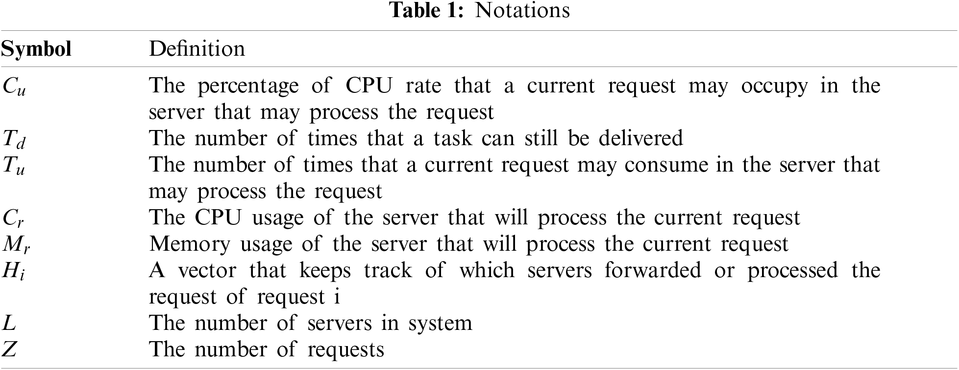
The request has two parts of attributes, Request itself and Server status. The first, request itself has three factors that are CPU Usage, deliver Time, using Time which stand for the percentage of CPU rate that current request may occupy in the server that may process the request, the number of times that a task can still be delivered, the times that a current request may consume in the server that may process the request, respectively. We use Cu to denote CPU Usage, Td to denote deliver Time and Tu to denote using Time. The second, server status has two factors that are CPU Rate and memeory Rate which stand for the CPU usage of the server that will process the current request and memory usage of the server that will process the current request. We use Cr to denote CPU Rate and Mr to denote memeory Rate. Finally, it has a vector Hi to keep track of which servers forwarded or processed the request, which i represents the current request.

2.1.2 Server Information

As mentioned above, each server has a virtual connection, which means both servers can send and receive requests from each other. We assume that each delivery between two server has a constant spend. Besides, each server has a vector R to record the status of connections to other nodes and the length of R is L, the number of server in our system.

After we build up our server and send requests to servers, we aim to schedule those requests to the right server to process and minimize the whole system cost according to every server status. In order to achieve both goals, we propose DLTSA to accomplish it.

2.2 DLTSA: Deep Learning-Based Traffic Scheduling Approach

DLTSA can deal with the problems mentioned in Section 4, which is easily implied. Particularly, the architecture of DLTSA system is given in Fig. 1. DLTSA can be divided into three modules: prepare module, judge module and process module. As you can see in Fig. 1, DLTSA system is a flexible distributed system. You can flexibly add and remove nodes in the system to achieve flexible deployment of edge servers to better provide service to IoT devices. Initially, the IoT devices will send request i to the server j in the area where the IoT device is located, and the request contains {Cu,Tu} mentioned above. Next, we will describe what the server will do.

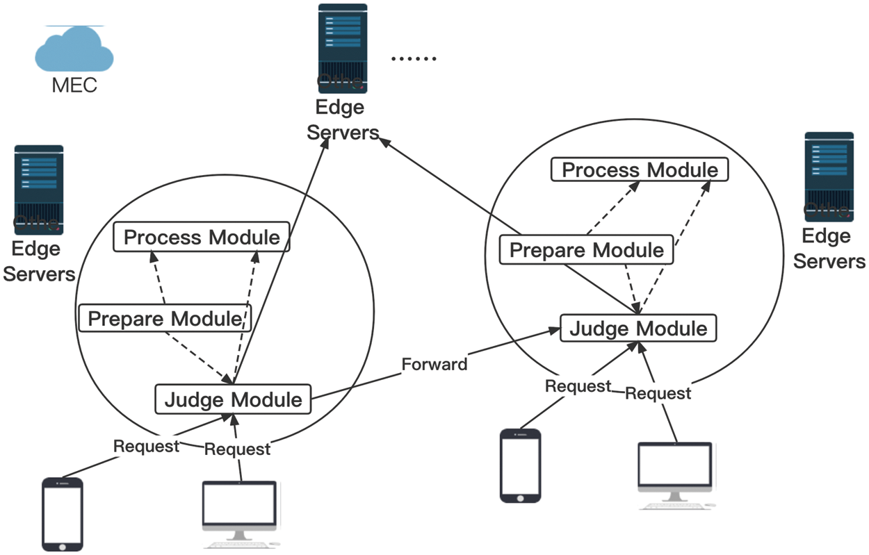
Figure 1: System framework

2.2.1 Implementation of Prepare Module

After receiving the request i, the prepare module in server j will first check whether the request has Td, if not, server will give a default threshold Dt to the request. If yes, the prepare module will check whether Td equals to zero, if yes it will send the request to the process module directly. Then the prepare module extracts Hi and Rj, and generate a relative complement Fu of Hi and Rj. Fu records the servers which the current server can send to. If Fu is empty, prepare module will send the request to process module. Next, the prepare module will obtain the local CPU rate and memory rate of server j and encapsulate those two factors with Cu, Tu, Td into a vector I, and the representation of I is:

I={Cu,Td,Tu,Cr,Mr}. (1)

Then, the server will send this vector to the scheduling module. The scheduling module will decide whether this server can process the request (call business service) or send it to another server. Finally, we give a constraint here:

Dt<=η, (2)

where η denotes the number of servers in the system. We can make sure the request will eventually be processed by the system with this constrain.

2.2.2 Implementation of Judge Module

Judge module is implemented by a two-layer fully connected neural network (NN), we use vector (1) which contains Cu, Td, Tu, Cr, Mr as input to the NN. In the hidden layer we have ten neurons and in the output layer we have one neuron. We use ReLu as our activation function, MSE as the loss function and SGD to update our weight. The structure of NN is shown in Fig. 2. If the result from the NN is greater than zero, the judge module will generate a boolean variable which value is true. Then the judge module will put the flag of the current server into Hi and send the request to other server which is in Fu. In reverse,the judge module will generate a boolean variable which value is false. Then it will send the request to process module. We use NN(⋅) to denote the judge function, and we use Forward(I, Fu) to denote the forward process.

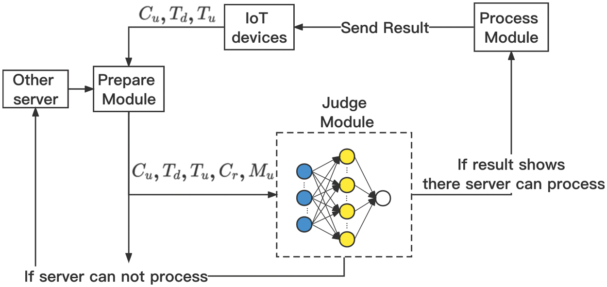
Figure 2: NN structure

At last, we summarize DLTSA in Algorithm 1. With the algorithm we can schedule each request to the right server. Besides with the output, we can know which server finally processed the request and which server forwarded the request and then we can calculate the cost of whole system.

2.3 Cost

As we describe in Section 2.2, the requests will be processed in two ways, either being processed directly or forwarded before being processed. In the second case where requests need to be forwarded, we assume that the network between each node is in the same condition (if two servers have connection with each other). And the delivery speed rate is Sd, request size is Ps, energy consumption per unit time of transmission is Cd, so the consumption of delivering one request from one server to another per times is:

Ce=Ps/Sd∗Cd. (3)

We use μ which is a 0–1 variable to denote whether the request has been delivered before. Then we generate a 1 by L matrix Mi according to Hi. In matrix Mi, we label the location of the server that appears in set Hi as 1; the remaining are 0. Also, we generate a 1 by L matrix Mo of all ones, next we can get the number of requests forwarded Ft:

Ft=Mi∗MoT. (4)

Above all, we can calculate delivery cost of request i:

Cfi=μ∗Ce∗Ft. (5)

Finally, we use Z to denote number of requests, then we get can get total transmission cost of system:

p=∑i=1ZCfi. (6)

We assume that the servers can process multiple requests in parallel and the sever starts to process requests after receiving all parts of a request. The server has two statuses-standby and working. Once the server receives the request then it will turn standby status to working status. We assume that once server goes to working status, it will try its best to provide the service, so we use Wb and Wu to represent the consumption of server per unit time. In the context of this article, Wb and Wu equal to 10W per minute, and 1 W per minute. We use θ to denote the status of the server. The total server cost is shown below:

v=∑i=1LT∗(θ∗Wb+(1−θ)∗Wu). (7)

At last, we can get the total system cost:

Totalcost=p+v. (8)

3  Evaluation

In this section, we evaluate the DLTSA algorithm. The effects of a different number of request sent to DLTSA and different number of servers in DLTSA are analyzed, and comparison experiments validate the effectiveness of the DLTSA algorithm. The servers are set at each region and there is only one server in each region, and each region has an average of fifty IoT devices. In the experiments, we consider two types of IoT devices, namely laptop, mobile phone and both of them can send requests to server according to their demands. We assume that requests come evenly, and every server can process requests parallelly. The size of each request is uniformly distributed in [0.9,1] Mb, the cost of delivery per second is 1W, and the delivery rate is 10Mb per second. Besides, the IoT devices will send 50 requests to the server per 0.1 s. As we mentioned above, the judge module is implied by an NN, and to train our NN, we use the data from Google trace [29]. We mark those tasks as requiring forwarding when the server CPU usage exceeds 70% and memory usage reaches 100%; these task data are randomly divided into training sets and verification sets to train and verify our neural network.

3.1 Effect of Number of Server in System and Requests

Figs. 3 and 4 show the effect of the numbers of servers in the system and requests on delivery cost and total cost. From the vertical view, we can see a different number of servers will lead to different performance of the system. This is because different node number can lead to a different server connection situation so as to bring different node selection in the process of forwarding. We can choose different number of nodes to deployed in a production environment according to different actual situation. Then, from the horizontal view we can see as the number of request increases, the total cost and delivery cost is also increasing. The reason is that the number of requests which need to be forwarded will also increase accordingly.

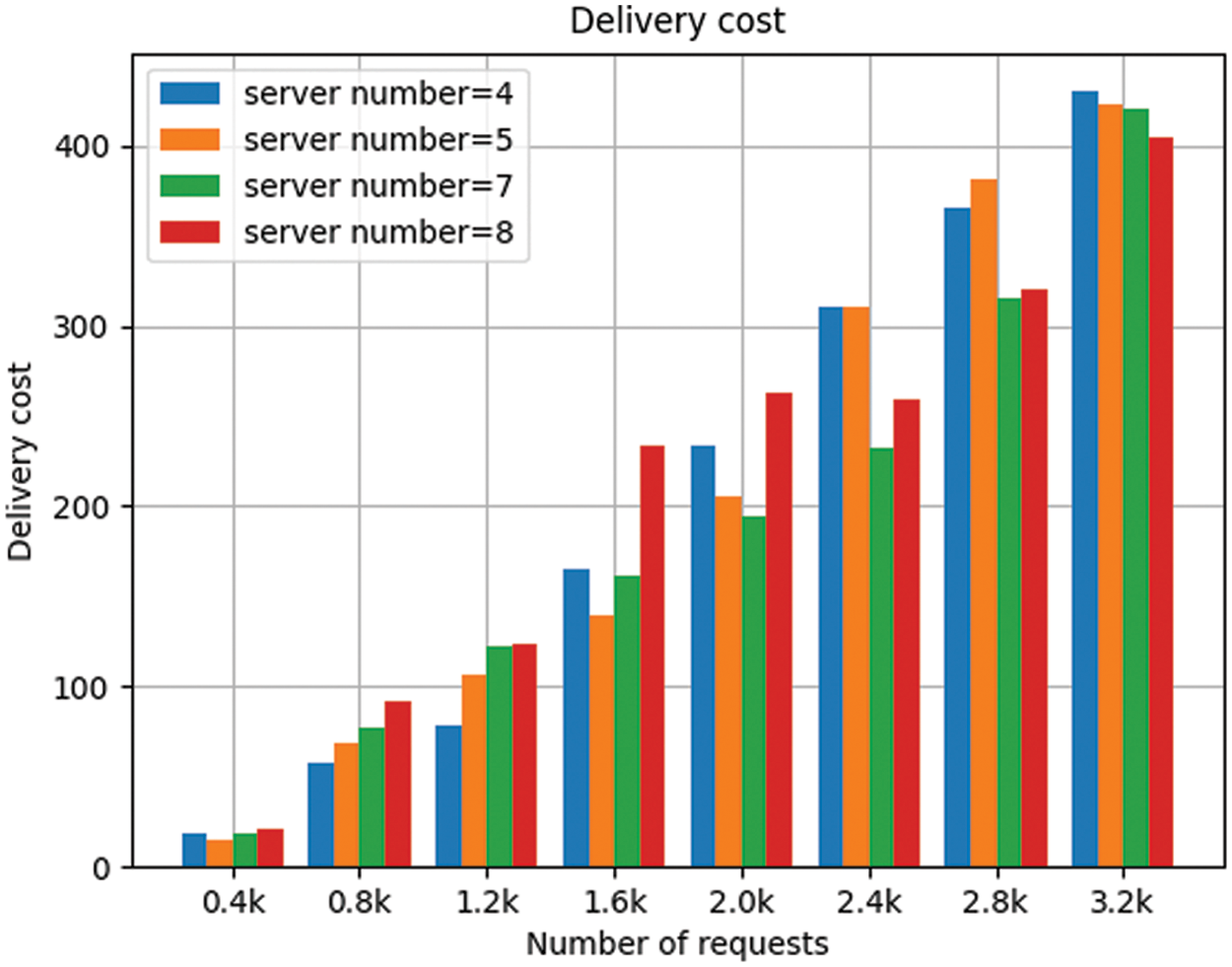
Figure 3: Delivery cost for different number of servers

Figure 4: Total costs for different number of servers

3.2 Comparison Experiment

In order to evaluate the effective performance of the DLTSA algorithm, we compare it with the other two algorithms.

Roundrobin algorithm: In each server, requests are assigned in polling to other servers which current server is connecting (could be it self). In the actual scenario of the random scheduling algorithm, the prepare module of DLTSA system is not change, but the judge module is removed by roundrobin algorithm.

Random scheduling algorithm: In each server, requests are randomly assigned to other servers which current server is connecting (could be it self). In the actual scenario of the random scheduling algorithm, the prepare module of DLTSA system is not change, but the judge module is removed by random scheduling algorithm.

Next, we compare and analyze the three algorithms from two performances metrics: Total cost and delivery cost and with a different number of server in the system.

We set up 4, 5, 7, 8 servers respectively in the system and let IoT devices send requests at intervals of 0.4k from 0k to 3.2k, then we collect processing information. From Figs. 5 to 8, we can see that as the number of requests increases, the delivery cost consumed by the system is increasing. This is because when the number of requests increases, the number of requests which need to be forwarded increases accordingly, resulting in the increase in delivery energy consumption. From Figs. 5 to 8, we can see that in each number of requests and each number of servers in the system, the delivery cost consumed by DLTSA algorithm is smaller than the delivery cost required by Random scheduling algorithm and Roundrobin algorithm. That shows DLTSA algorithm outperforms in saving the delivery cost of the MEC system. This is because, in contrast to random and polling algorithms, DLTSA does not simply send requests to other servers, but processes them themselves when they are not necessary. When the number of requests exceeds the capacity of the current server, the request is forwarded and other servers try to process it. The DLTSA algorithm effectively reduces the delivery cost of the whole system.

Figure 5: Delivery cost of 5 servers

Figure 6: Delivery cost of 5 servers

Figure 7: Delivery cost of 7 servers

Figure 8: Delivery cost of 8 servers

From Fig. 9 to Fig. 12, we can also see that in each number of requests and each number of servers in the system, the total cost consumed by DLTSA algorithm is smaller than the total cost required by Random scheduling algorithm and Roundrobin algorithm. This is because compared to random and roundrobin algorithms, DLTSA does not forward requests to other servers if it has enough processing power. Those servers that do not have requests are not needed to be started, they will stay in standby status. But for random algorithms, each server has a chance to receive and process a request. And for roundrobin algorithms, each server will always get a turn to receive and process a request. For those two algorithms, the servers in system will always in Startup mode. Thus, our DLTSA algorithm can effectively reduce the system cost. Besides, although it can be seen that there is a surge from 1.2k to 1.6k in 4-node system and 8-node system, and a surge from 2.0k to 2.4k in 5-node system. But on the whole, the delivery cost and total cost of DLTSA algorithm will converge as the number of requests increases.

Figure 9: Total cost of 4 servers

Figure 10: Total cost of 5 servers

Figure 11: Total cost of 7 servers

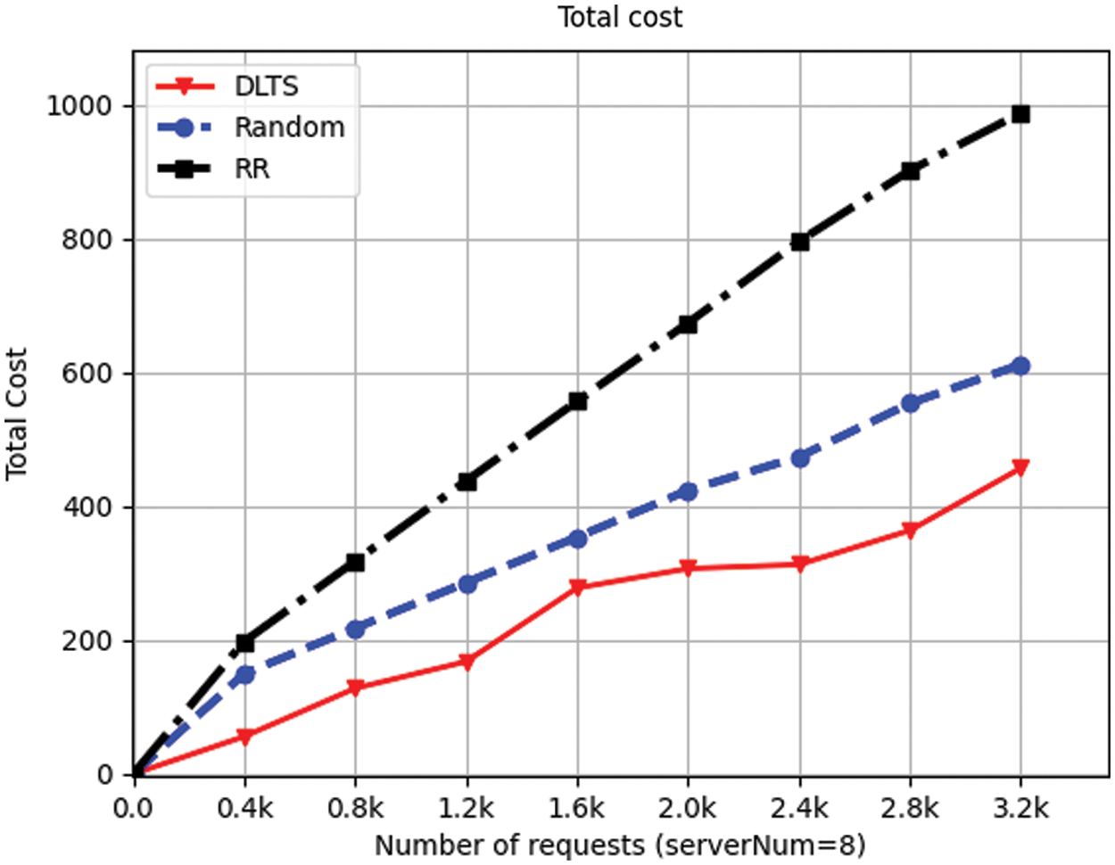
Figure 12: Total cost of 8 servers

Then we compare and analyze the number of tasks delivered by the three algorithms with different number of requests and different number of server in system.

Figs. 13 to 16 show that the task average delivery times of three algorithm with different number of requests and different number of servers. Taking the first column in Fig. 13 as an example, task average delivery times refers to the average number of tasks be delivered in the system when the number of servers in the system is 4 and the number of tasks received is 0.4k. The smaller the value is, the fewer times the task is delivered, that is, the task is more likely to be processed by the local machine. From Figs. 13 to 16, we can see that under different number of servers and different requests, the task average delivery times of our method is smaller than that of the other two methods. This is because the traditional random and the RR algorithm tend to divide all requests equally between each edge server, so that each server is allocated some request processing. But these two algorithms miss a key point: they do not use up every server’s performance. In contrast, the task average delivery times of our algorithm in each case are smaller than those of the two algorithms, which means that our algorithm better considers the performance of each server and determines whether to forward the task according to each edge server performance.

Figure 13: Average delivery times (serverNum = 4)

Figure 14: Average delivery times (serverNum = 5)

Figure 15: Average delivery times (serverNum = 7)

Figure 16: Average delivery times (serverNum = 8)

From Figs. 13 to 16, we can also see that no matter how many servers there are in the system, our algorithm shows a convergence trend in the task average delivery times when the number of requests increases. In other words, the average delivery times growth rate decreases as the number of requests increases. In system of eight servers (Fig. 16), there is a negative growth as the number of requests increased. This is because there is a potential adaptive adjustment in our algorithm that allows a server to expand the list of servers which can be sent when the server load is high for a while. In this way, each times the current server decides to forward a task, the task can be sent to more servers, allowing more servers to serve it. When the server load is down, we remove the redundant servers from the list of available servers. By using this way, service redundancy is avoided and the number of delivering tasks does not increase as the number of requests increases, ensuring the stability of the system. However, the traditional random and RR algorithms cannot do this. These two methods will make all servers in a hot state, resulting in an increase of the task average delivery times and an increase the energy consumption of the system.

Finally, we compare and analyze the total task transmission delay of the three algorithms with different request number and different number of server in system.

Figs. 17 to 20 show that the total task transmission delay of three algorithm with different request number and different number of server. The total task transmission delay is the sum of each task transmission delay. Task transmission delay represents the time it takes for each task to be forwarded in the system. The lower the transmission delay, the less time it takes for each task to be forwarded in the system. In other words, the lower the transmission delay of tasks, the earlier each task is processed by the system servers and the earlier the results are returned to the user to provide better quality of service (QoS).

Figure 17: Total transmission delay (serverNum = 4)

Figure 18: Total transmission delay (serverNum = 5)

Figure 19: Total transmission delay (serverNum = 7)

Figure 20: Total transmission delay (serverNum = 8)

As can be seen from Figs. 17 to 20, under a different number of servers and a different number of requests, the task transmission delay in our method is much lower than that of random algorithm and RR algorithm. This is because, for random algorithm and RR algorithm, their goal is to ensure the fairness of each server in the system, hoping to minimize the variance of the number of tasks per server. But they ignore that it takes time for tasks to be delivered between server nodes. The fundamental purpose of task scheduling is to make the task be processed within the expected time of the user, but the random and RR algorithms do not take this into account, resulting in the task not being processed faster, and the task processing results cannot be returned to the user in time.

From Figs. 17 to 20, we can also see that, in general, the growth rate of task transmission delay actually decreases as the number of requests increases regardless of the number of servers in the system. This shows that our system becomes more stable as more requests increase. Meanwhile, if we observe from Figs. 17 to 20, when our algorithm is faced with a high volume requests like 3.2k (the last column in Figs. 17 to 20), the task transmission delay tends to decrease. This means that our algorithm will not increase the transmission delay due to the increase in the number of servers in the system. On the contrary, our algorithm will fully consider the user’s quality of service, make a more reasonable choice on task scheduling, and make full use of existing resources to process tasks while ensuring the task completion time.

In summary, as shown in Figs. 5 to 12, we can obtain a conclusion that DLTSA algorithm has a good performance on minimizing the total scheduling cost. From Figs. 13 to 16, we can see that DLTSA can effectively reduce the average forwarding times of tasks and achieve global optimization by separately considering the status of each server. From Figs. 17 to 20, we know that DLTSA also makes tasks to be processed more effectively and helps maintaining the stability of the MEC system.

4  Related Work

SAMI [16] leverages Service Oriented Architecture (SOA) to propose an arbitrated multi-tier infrastructure model for MCC. SAMI allocate services with suitable resources according to several metrics. Using SAMI can facilitate development and deployment of service-based platform-neutral mobile applications. You et al. [17] proposed an energy efficient computing framework. This framework translated policy optimization problem into equivalent problems of minimizing the mobile energy consumption for local computing and maximizing the mobile energy savings for offloading. And this framework demonstrated that MCC is better than local computing.

Some methods had been proposed to solve the scheduling problem in MEC. Wu et al. [18] proposed a task offloading method. This method uses DQN to learn offloading strategy at each user equipment. Meanwhile, this method uses optimization algorithm to allocate communication resources at each computational access point. Dinh et al. [20] proved that Mobile Users (MUs) could achieve a Nash equilibrium via a best response-based offloading mechanism. They proposed a model-free reinforcement learning offloading mechanism which helps MUs learn their long-term offloading strategies to maximize their long-term utilities.

Some efforts have been devoted to improving the efficiency of MEC from an energy aspect. To minimize energy cost for a multi-cell multi-user MEC system, MIMO [30] ignores offloading decision making that each of the UEs was assumed to offload its task to a specific server. But it does not take into account server capacity when requests surge in an area, it cannot send tasks from one server the others. Chen et al. [16] put forward a distributed task offloading scheme based on game theory. But it requires each user to frequently obtain information of communication resources and calculation resources from MEC server rather than send tasks to the server and let the server do the scheduling. That will cause great energy consumption burden to IoT devices. Ebrahimzadeh et al. [31] considered using distributed cooperative algorithm in multi-user scenario, combined with wireless power, MEC server resource allocation and communication resource allocation to reduce user energy consumption. However, the additional computing resource consumption by this method is also high.

Recently, deep learning has been applied to solve a variety of problems in classification, e.g., [32,33]. The above methods all consider the task processing attribution of IoT devices and servers and take the entire system into account. But all servers are involved in processing all the tasks rather than having a balance between IoT devices processing tasks the servers processing the tasks. And if we consider each server status in MEC [34], the scheduling problem can be formed as a classification problem for a server to process a task or forward the task to another server. By using the neural network, we take server status and request task information as input to get classification results and build a totally distributed system. It is a novel idea which aims to solve the scheduling problem and workload problem in MEC.

5  Conclusion

In this work, we first gave some previous scheduling strategies in MEC and put forward some related problems. Based on the observations, we considered a multi-server MEC network, formulated these problems to a distributed multi-server MEC system without considering IoT devices processing capacity. We proposed a deep Learning-Based algorithm embedded in a traffic scheduling system. We used server status and request information as the input to build a neural network. And we used that neural network to decide whether the server can process the request itself or let other servers do. Then we gave a method to calculate the cost. We used that method to evaluate the proposed DLTSA by setting different numbers of server and different numbers of request. Then we compare total cost and delivery cost with two traditional distributed algorithms. Experimental results showed that DLTSA significantly outperforms the baselines with cost saving in MEC.

Funding Statement: This work was supported in part by the National Natural Science Foundation of China (61902029), R&D Program of Beijing Municipal Education Commission (No. KM202011232015), Project for Acceleration of University Classification Development (Nos. 5112211036, 5112211037, 5112211038).

Conflicts of Interest: The authors declare that they have no conflicts of interest to report regarding the present study.

References

Armbrust, M., Fox, A., Griffith, R., Joseph, A. D., Katz, R. et al. (2010). A view of cloud computing. Communications of the ACM, 53(4), 50–58. DOI 10.1145/1721654.1721672. [Google Scholar] [CrossRef]

Tan, L., Wang, N. (2010). Future internet: The Internet of Things. 3rd International Conference on Advanced Computer Theory and Engineering (ICACTE), pp. 376–380. Chengdu, China. [Google Scholar]

Qi, L., Yang, Y., Zhou, X., Rafique, W., Ma, J. (2021). Fast anomaly identification based on multi-aspect data streams for intelligent intrusion detection toward secure Industry 4.0. IEEE Transactions on Industrial Informatics, 18(9), 6503–6511. [Google Scholar]

Wang, F., Li, J. S., Wang, Y. L., Rafique, W., Khosravi, M. R. et al. (2022). Privacy-aware traffic flow prediction based on multi-party sensor data with zero trust in smart city. ACM Transactions on Internet Technology. [Google Scholar]

Huang, J., Zhang, C., Zhang, J. (2020). A multi-queue approach of energy efficient task scheduling for sensor hubs. Chinese Journal of Electronics, 29(2), 242–247. DOI 10.1049/cje.2020.02.001. [Google Scholar] [CrossRef]

Chen, X., Jiao, L., Li, W., Fu, X. (2016). Efficient multi-user computation offloading for mobile-edge cloud computing. IEEE/ACM Transactions on Networking, 24(5), 2795–2808. DOI 10.1109/TNET.2015.2487344. [Google Scholar] [CrossRef]

Xu, J., Li, D., Gu, W., Chen, Y. (2022). UAV-assisted task offloading for IoT in smart buildings and environment via deep reinforcement learning. Building and Environment, 2022, 109218. DOI 10.1016/j.buildenv.2022.109218. [Google Scholar] [CrossRef]

Chen, Y., Gu, W., Li, K. (2022). Dynamic task offloading for internet of things in mobile edge computing via deep reinforcement learning. International Journal of Communication Systems. DOI 10.1002/dac.5154. [Google Scholar] [CrossRef]

Huang, J., Tong, Z., Feng, Z. (2022). Geographical POI recommendation for internet of things: A federated learning approach using matrix factorization. International Journal of Communication Systems. DOI 10.1002/dac.5161. [Google Scholar] [CrossRef]

Zhang, Y., Wang, K., He, Q., Chen, F., Deng, S. et al. (2021). Covering-based web service quality prediction via neighborhood-aware matrix factorization. IEEE Transactions on Services Computing, 14(5), 1333–1344. DOI 10.1109/TSC.2019.2891517. [Google Scholar] [CrossRef]

Chen, Y., Liu, Z., Zhang, Y., Wu, Y., Chen, X. et al. (2021). Deep reinforcement Learning-Based dynamic resource management for mobile edge computing in industrial Internet of Things. IEEE Transactions on Industrial Informatics, 17(7), 4925–4934. DOI 10.1109/TII.2020.3028963. [Google Scholar] [CrossRef]

Cuervo, E., Balasubramanian, A., Cho, D. K., Wolman, A., Saroiu, S. et al. (2010). Maui: Making smartphones last longer with code offload. Proceedings of the 8th International Conference on Mobile Systems, Applications, and Services, New York, NY, USA. [Google Scholar]

Lu, Y., Chen, Y., Liu, Z., Zhang, Y. (2022). Cost-efficient resources scheduling for mobile edge computing in ultra-dense networks. IEEE Transactions on Network and Service Management. DOI 10.1109/TNSM.2022.3163297. [Google Scholar] [CrossRef]

Sanaei, Z., Abolfazli, S., Gani, A., Buyya, R. (2014). Heterogeneity in mobile cloud computing: Taxonomy and open challenges. IEEE Communications Surveys Tutorials, 16(1), 369–392. DOI 10.1109/SURV.2013.050113.00090. [Google Scholar] [CrossRef]

Buyya, R., Yeo, C. S., Venugopal, S. (2008). Market-oriented cloud computing: Vision, hype, and reality for delivering it services as computing utilities. 2008 10th IEEE International Conference on High Performance Computing and Communications, pp. 5–13. Dalian, China. [Google Scholar]

Sanaei, Z., Abolfazli, S., Gani, A., Shiraz, M. (2012). Sami: Service-based arbitrated multi-tier infrastructure for mobile cloud computing. 2012 1st IEEE International Conference on Communications in China Workshops (ICCC), pp. 14–19. Beijing, China. [Google Scholar]

You, C., Huang, K., Chae, H. (2016). Energy efficient mobile cloud computing powered by wireless energy transfer. IEEE Journal on Selected Areas in Communications, 34(5), 1757–1771. DOI 10.1109/JSAC.2016.2545382. [Google Scholar] [CrossRef]

Wu, Y. C., Dinh, T. Q., Fu, Y., Lin, C., Quek, T. Q. S. (2021). A hybrid DQN and optimization approach for strategy and resource allocation in MEC networks. IEEE Transactions on Wireless Communications, 20(7), 4282–4295. DOI 10.1109/TWC.2021.3057882. [Google Scholar] [CrossRef]

Shi, W., Cao, J., Zhang, Q., Li, Y., Xu, L. (2016). Edge computing: Vision and challenges. IEEE Internet of Things Journal, 3(5), 637–646. DOI 10.1109/JIOT.2016.2579198. [Google Scholar] [CrossRef]

Dinh, T. Q., La, Q. D., Quek, T. Q. S., Shin, H. (2018). Learning for computation offloading in mobile edge computing. IEEE Transactions on Communications, 66(12), 6353–6367. DOI 10.1109/TCOMM.2018.2866572. [Google Scholar] [CrossRef]

Chen, Y., Xing, H., Ma, Z., Chen, X., Huang, J. (2022). Cost-efficient edge caching for noma-enabled IoT services. China Communications. [Google Scholar]

Global Cloud Index (2018). Forecast and methodology, 2016–2021 white paper. [Google Scholar]

Chen, Y., Zhao, F., Lu, Y., Chen, X. (2021). Dynamic task offloading for mobile edge computing with hybrid energy supply. Tsinghua Science and Technology. DOI 10.26599/TST.2021.9010050. [Google Scholar] [CrossRef]

Huang, J., Lv, B., Wu, Y., Chen, Y., Shen, X. (2022). Dynamic admission control and resource allocation for mobile edge computing enabled small cell network. IEEE Transactions on Vehicular Technology, 71(2), 1964–1973. DOI 10.1109/TVT.2021.3133696. [Google Scholar] [CrossRef]

Chen, Y., Zhao, F., Chen, X., Wu, Y. (2022). Efficient multi-vehicle task offloading for mobile edge computing in 6G networks. IEEE Transactions on Vehicular Technology, 71(5), 4584–4595. DOI 10.1109/TVT.2021.3133586. [Google Scholar] [CrossRef]

Satyanarayanan, M. (2017). The emergence of edge computing. Computer, 50(1), 30–39. DOI 10.1109/MC.2017.9. [Google Scholar] [CrossRef]

Xu, X., Fang, Z., Zhang, J., He, Q., Yu, D. et al. (2021). Edge content caching with deep spatiotemporal residual network for iov in smart city. ACM Transactions on Sensor Networks, 17(3), 1–33. DOI 10.1145/3447032. [Google Scholar] [CrossRef]

Qi, L., Hu, C., Zhang, X., Khosravi, M. R., Sharma, S. et al. (2020). Privacy-aware data fusion and prediction with spatial-temporal context for smart city industrial environment. IEEE Transactions on Industrial Informatics, 17(6), 4159–4167. DOI 10.1109/TII.9424. [Google Scholar] [CrossRef]

Cloud, G. (2011). Google cloud trace data. [Google Scholar]

Sardellitti, S., Scutari, G., Barbarossa, S. (2014). Joint optimization of radio and computational resources for multicell mobile cloud computing. 2014 IEEE 15th International Workshop on Signal Processing Advances in Wireless Communications (SPAWC), Toronto, ON, Canada. DOI 10.1109/SPAWC.2014.6941749. [Google Scholar] [CrossRef]

Ebrahimzadeh, A., Maier, M. (2019). Distributed cooperative computation offloading in multi-access edge computing fiber-wireless networks. Optics Communications, 452, 130–139. DOI 10.1016/j.optcom.2019.06.060. [Google Scholar]

Zhao, P., Hou, L., Wu, O. (2020). Modeling sentiment dependencies with graph convolutional networks for aspect-level sentiment classification. Knowledge-Based Systems, 193, 105443. DOI 10.1016/j.knosys.2019.105443. [Google Scholar] [CrossRef]

Xu, X., Tian, H., Zhang, X., Qi, L., He, Q. et al. (2022). Discov: Distributed COVID-19 detection on X-ray images with edge-cloud collaboration. IEEE Transactions on Services Computing, 15(3), 1206–1219. DOI 10.1109/TSC.2022.3142265 [Google Scholar] [CrossRef]

Zhang, Y., Pan, J., Qi, L., He, Q. (2021). Privacy-preserving quality prediction for edge-based IoT services. Future Generation Computer Systems, 114, 336–348. DOI 10.1016/j.future.2020.08.014. [Google Scholar] [CrossRef]