A Dynamic Maintenance Strategy for Multi-Component Systems Using a Genetic Algorithm

Nomenclature

1  Introduction

As reliability, availability, maintainability and safety are integrated into the traditional maintenance process, people tend to strengthen their ability to predict faults by using the knowledge of the component conditions to take appropriate preventive measures to reduce costs and risks [1–3]. In this context, prognostics and health management (PHM) is playing an increasingly important role. PHM can be combined with multiple disciplines, such as machine learning [4,5] sensor technology [6,7], fault diagnosis [8], statistics [9–12] and reliability engineering [13–16], to realize an online evaluation of system health status and to predict the state of the system based on the current information. PHM converts signals and data detected by sensors into health status information about the system, and it alerts users so that the system can be maintained in a timely manner.

The performance of the components in a system will gradually deteriorate over time [15–17]. Therefore, people need to maintain systems periodically to ensure the function. It is desirable for a maintenance plan to be performed as accurately as possible to achieve optimal cost. In fact, the degradation state of systems changes dynamically, so it is difficult to perform accurate maintenance plans, especially for rotary structures [18–20]. In view of the disadvantages of the existing maintenance policies, a new condition-based maintenance (CBM) strategy is proposed based on PHM, which performs according to the analysis and prediction results of system degradation parameters. In CBM, maintainers can collect sensor data to identify the current system health status. On the basis of CBM, predictive maintenance (PdM) is developed. The CBM strategy only replaces or repairs a damaged part, reducing the cost of the system in the whole life cycle. Maintainers can schedule an appropriate strategy for each device or a single component or subsystem based on the predicted degradation state, then select an appropriate replacement or inspection cycle.

A lot of work with different strategies based on the data and assumptions has been done to solve these issues. Susto et al. [21] proposed a multi-classifier PdM system for integrated faults. Working in parallel with multiple machine learning classifiers, the knowledge of tools/logical variables was renewed in each iteration to enhance decisions, which improved maintenance management decisions to minimize operating costs. Schmidt et al. [22] achieved an improvement in PdM decision-making through a cloud-based approach with the use of wide information content. Wei et al. [23] proposed a CBM strategy that determined the optimal operation according to the system state to minimize the average long-run cost rate. Zhang et al. [24] classified the industrial applications of PdM based on machine learning and deep learning algorithms, compared the performance metrics of each classification such as signal type, application scenario, target, accuracy and data source, and evaluated the metrics of each PdM algorithm. Chen et al. [25] proposed a maintenance decision method considering performance degradation, which determined the optimal time to conduct maintenance activities through an online evaluation of maintenance costs. Theissler et al. [26] proposed a maintenance strategy for automotive systems based on machine learning methods that could ensure product functional safety and control maintenance costs in the life cycle. Ayvaz et al. [27] developed a data-driven predictive maintenance system for manufacturing production lines. Acquiring data generated in real time from IoT sensors, the system aimed to detect signals before potential failures through machine learning methods so that preventive measures could be taken before production was shut down. Arena et al. [28] developed a PdM strategy based on a decision tree, which took into account environmental awareness information, the maturity of the collected data, the detectability of potential failures, and direct and indirect maintenance costs.

In the preventive maintenance activities of multi-component systems, the maintenance strategy of a single component system is often used to determine the maintenance interval, ignoring the dependency between components in the multi-component system. For multi-component systems, it is unreasonable to assume that the components are independent, which means that maintenance strategies may not be the optimal choice at the time. Therefore, to introduce multi-component dependencies in preventive maintenance policies, multi-component systems need grouping. Grouping is a common maintenance strategy for multi-component systems with an arbitrary combination of series and parallel structures.

The existing maintenance strategies mainly have the following problems:

(1)   It is difficult to find the optimal grouping: complex structures may have positive and negative effects on maintenance grouping. In addition, an inappropriate group may lead to higher economic and time costs;

(2)   Only the impact of the critical components on the systems is considered. However, the importance of other components in the structure when they fail is ignored.

This paper proposes a maintenance strategy based on structure dependency for multi-component system PdM:

(1)   The maintenance strategy minimizes the expected depreciation cost of the system and selects the optimal maintenance strategy for each component or subsystem;

(2)   Aiming at the non-deterministic polynomial (NP)-complete problem in the optimization of multi-component system maintenance grouping strategy, a random allocation scheme based on a genetic algorithm is proposed to find the optimal grouping;

(3)   In this paper, an 11-component gearbox system is taken as an example to illustrate the effectiveness of the maintenance strategy, and the influence of the system structure, maintenance cycle and initial parameters on the maintenance strategy is discussed.

2  Multi-Component Grouping Model

It is a difficult task to choose the right maintenance strategy for each device, component or subset in a complex system. In order to minimize the maintenance costs of the entire industrial system under operating conditions, it is necessary to develop an operation plan for each component and to choose the optimal time interval for system maintenance to meet the operator requirements for safety, reliability and economy.

2.1 Component Importance Indicator

We consider a system consisting of n independent components with a complex structure. The structure may contain an arbitrary series, parallel or series–parallel combination. In a multi-component system, especially in the case of a complex structure, it is necessary to determine which components are more “important”; that is, the components that have a more obvious impact on system reliability, availability, productivity, security, etc. [29]. Therefore, it is necessary to introduce a critical component to measure the importance of the components by structure. According to the characteristics of the system structure, the components of a system are divided into two types: critical components and non-critical components. If a component stops for some reason (such as a failure or maintenance operation) and the system then stops, this is called a critical component; a component is a non-critical component if its failure does not stop the system. For a system with n components, an indicator parameter is used to describe whether the ith (i=1,…,n) component is a critical component. When πi=0, the component is not a critical component, and the system will still work when this component stops (fails or is overhauled); when πi=1, the component is a critical component, and its stopping (failure or maintenance) will lead to the failure of the system. Based on the above definition, a critical component can be expressed as Eq. (1):

πi={0(when componentiis non-critical)1(when componentiis critical)(1)

However, using only a binary function to describe the importance of a component is not detailed enough. We take a multi-component series and a parallel system with eight components in Fig. 1 as an example. The number of components is n = 8 in this system. According to the definition of critical components, the system fails when components 1 and 8 stop. Therefore, components 1 and 8 are critical components, and the other components are non-critical components. π1=1,π2=0,π3=0, π4=0,π5=0,π6=0,π7=0,π8=1. Therefore, components 1 and 8 are structurally more important than the other components. When component 7 fails, components 2 and 6 become critical components, and when component 3 fails, components 4 and 5 become critical components. It is not enough to simply describe the importance of components with πi=0 and πi=1.

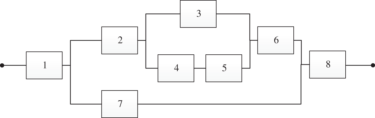
Figure 1: Reliability block diagram of a series and parallel multi-component system with 8 components

Therefore, this section uses the component importance indicator (CII) proposed in [30] to evaluate the importance of each component in the structure. The state vector y=(y1,…yi,…,yn) is used to describe the running state of each component. If the ith component is not running, then yi=0; if component i is running, then yi=1. Therefore, the operating state of the entire system is described as a binary function:

Φ(y)={0(when the system is running)1(when the system is stop running)(2)

Φ(y) is also known as the structural function of the system. A system that is functioning if, and only if, all its n-many components are functioning is called a series structure. A parallel structure function could be expressed by:

Φ(y)=∏i=1n(yi)(3)

A system that is functioning if at least one of its n-many components is functioning is called a parallel structure. A parallel structure function could be expressed by:

Φ(y)=1−∏i=1n(1−yi)(4)

Then, the component importance indicator of the ith component is defined as follows:

CIIi=ηΦ(i)2n−1(5)

where ηΦ(i) is the total number of critical vectors of the ith component.

ηΦ(i)=∑(i,x)[Φ(1i,y)−Φ(0i,y)](6)

where Φ(1i,y) is all the possible state vector values in the system when the ith component runs; Φ(0i,y) is all the possible state vector values in the system when the ith component fails.

The component importance indicator in Fig. 1 is calculated from Eq. (5), as shown in Table 1.

2.2 Failure Probability of Components

The distribution of failure probability within the preventive maintenance cycle satisfies the two-parameter Weilbull distribution. For a system with i components, the system failure probability is defined as follows [31,32]:

pi(t)=ζiψi(tψi)ζi−1(7)

where ζ and ψ are shape and size parameters. Assume that when a component is replaced during a maintenance cycle, the degradation of that component is reset to 0. At this point, the failure probability of the component in the r maintenance cycle is rewritten as:

pi,r(t)=ζi,rψi,r(tψi,r)ζi,r−1(8)

where 0≤pi,r≤1. When the system failure probability pi,r is closer to 0, the system is healthier. When pi,r=0, the system is new; when pi,r=1, the system is faulty and cannot continue to work. ζi,r and ψi,r will increase with an increase in maintenance times r, which reflects the decline in system health in use. For the ith component that has undergone r times of maintenance, its failure probability function is expressed in a piecewise form, as shown in Fig. 2.

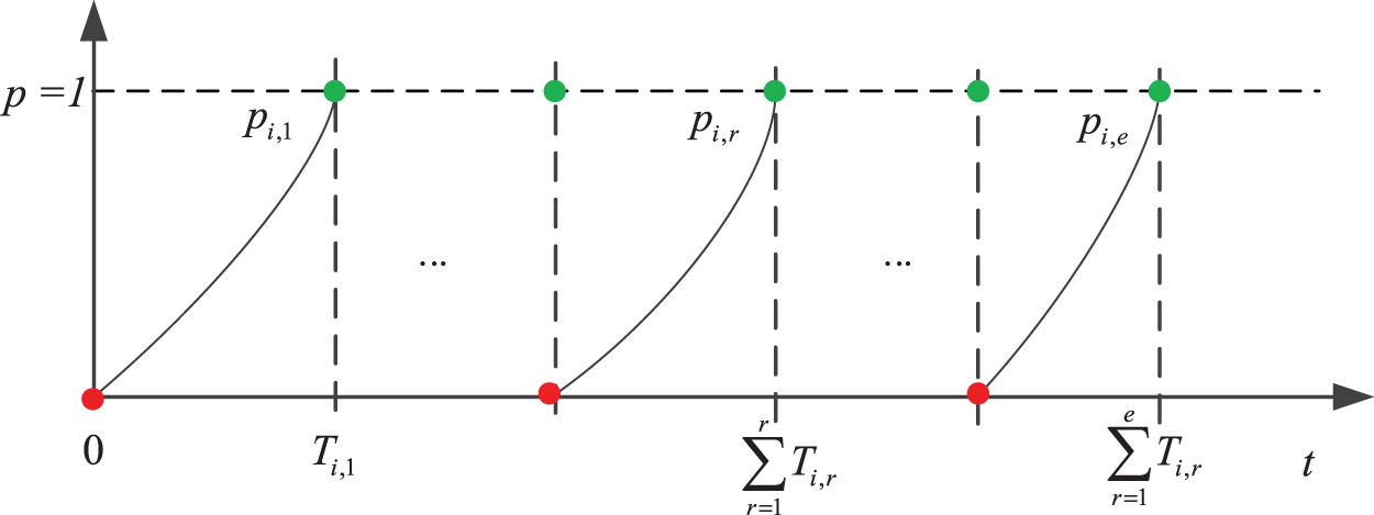
Figure 2: System failure rate after maintenance

The figure shows different maintenance activity cycles Ti,1,…,Ti,r…,Ti,e. As in the Fig. 2, after one maintenance cycle Ti,r, the failure probability of component i drops to 0, but the slope of the system failure probability curve increases. The system arrives at pi,r=1 at a faster “speed”, which leads to the shortening of the maintenance interval. This pattern is carried over into subsequent maintenance cycles; that is, components do not recover as a result of maintenance, but rather deteriorate over time.

In this study, the maximum likelihood method is used to identify the system failure parameters. The maximum likelihood estimation parameter is identified using the Newton iteration method.

2.3 Multi-Component Systems Grouping

In the previous multi-component system maintenance work, a maintenance strategy was proposed for a series system. A grouping strategy needs to find a proper balance between start-up cost, system failure cost and system structure to ensure the economic benefits of the whole system. Proper grouping can significantly reduce system maintenance costs [33].

The following assumptions are made for grouping:

Assumption 1: Assume that critical components and groups do not change during the maintenance cycles. The system structure does not change over time.

Assumption 2: Wear and fatigue are the main causes of industrial machinery equipment failure (rotary bearings, aircraft and marine engines) [34]. In this paper, it is assumed that each component is subject to fatigue mechanisms during its lifetime. The wear/fatigue process of components can be regarded as the degradation behavior of their health state.

Assumption 3: The entire system is maintained with sufficient human resources, and each component is maintained immediately without waiting for downtime.

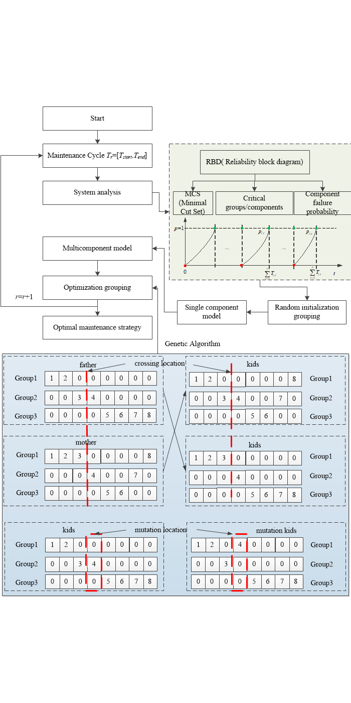
The reliability block diagram (RBD) describes the connection between components in a system, and shows the logical connections of the components needed to implement a particular system function. A set containing the minimum number of component failures sufficient to cause a system shutdown is called the minimal cut set (MCS). If the MCS contains ε components, then the MCS is ε order. If there is one or more critical component in a group, it is considered a critical group (CG); otherwise, it is not regarded as a critical group. The grouping process is shown in Fig. 3, where Tr is the rth maintenance cycle, r = 1, …, e and e is the number of maintenance cycles.

(1)   System analysis: the reliability block diagram is obtained, then relationship of the series and the parallel between multiple components is determined; the failure probability parameters are identified from component degradation status data.

(2)   Random initialization grouping: n components are randomly divided into N groups, including a total of L preventive maintenance activities. For arbitrary grouping, Gkand Gm (m≠k) meet the following conditions:

Gk∩Gm=∅(9)

(3)   Single component economic model: based on the failure probability of single component parameters and the expected maintenance cost model for a long period, a single component maintenance strategy is built. This strategy is built on the basis that each component is independent, which is a tentative maintenance strategy.

(4)   Muti-component economic model: based on the dependency and grouping of components, an optimal maintenance plan is calculated for randomly grouped multiple components in a maintenance cycle [Tstart, Tend].

(5)   Optimization of grouping: a genetic algorithm is used to find the appropriate grouping strategy to minimize the total cost of the preventive maintenance strategy for the whole system.

(6)   Update: the optimal time interval and grouping strategy are obtained in the current maintenance cycle Tr. When the current maintenance is complete, a new maintenance plan for Tr+1 is required. The cost of components in a system varies over time, and the degradation may be more dramatic. The maintenance strategy needs to change as these parameters change. To this end, the failure probability parameters of each component need to be renewed, and the degradation degree and cost of each component in the new maintenance cycle need to be updated r = r + 1. Steps 2–6 are performed and all maintenance cycles are iterated until r = e. The dynamic allocation of the maintenance strategy is implemented.

(7)   Outputting the optimal maintenance policy for each cycle.

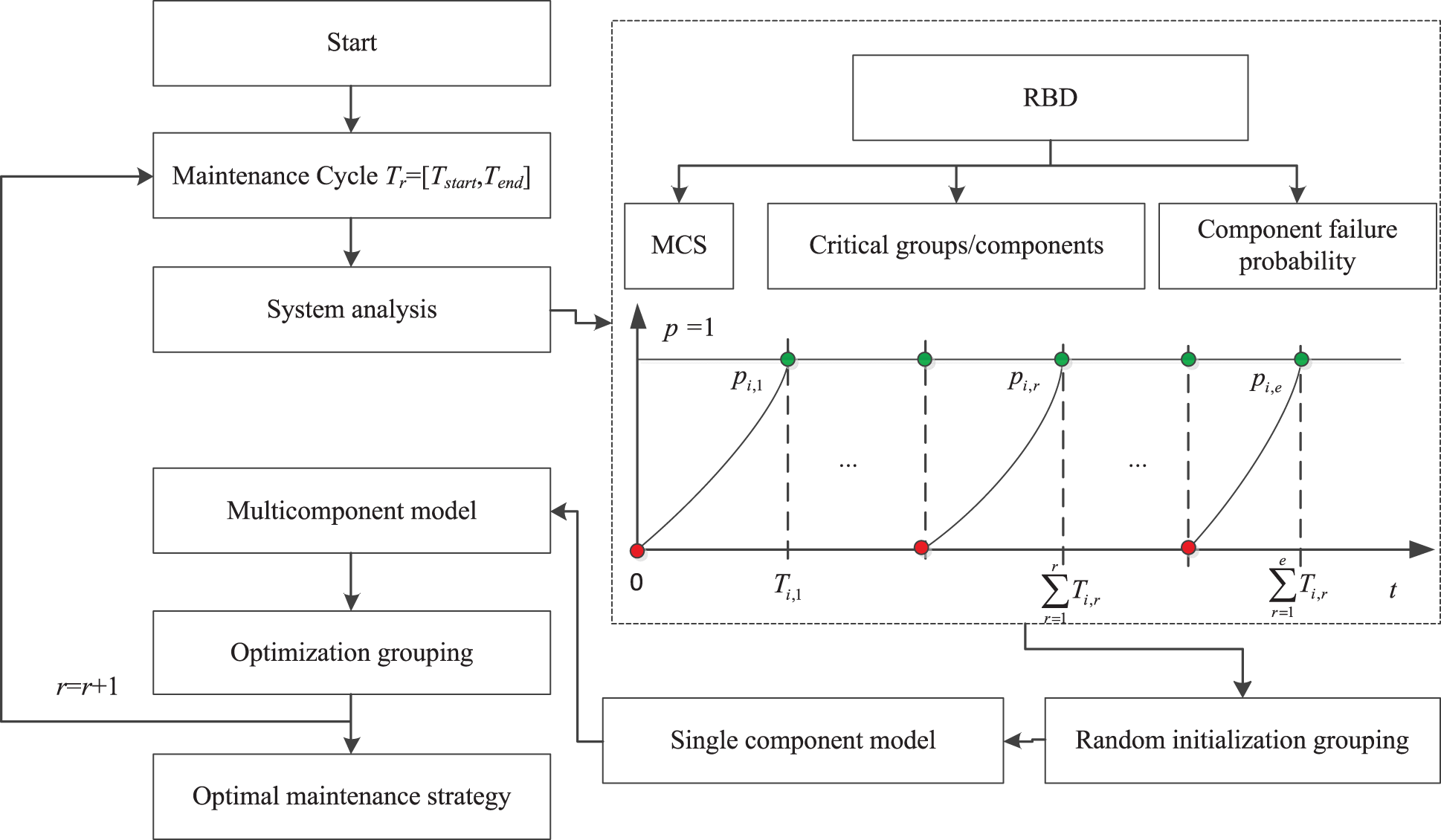
Figure 3: Multi-component systems grouping process

3  Maintenance Policies of Multi-Component System

In order to implement a preventive maintenance policy for multi-component systems, it is necessary to ensure the high reliability and integrity of the system under the preventive maintenance policy. From the perspective of reliability, the more groups and the more frequent maintenance that is undertaken, the better the reliability. However, this will lead to an increase in maintenance costs and a decrease in the available efficiency of the system, making this strategy impractical. Therefore, we propose a preventive maintenance strategy based on the grouping model. According to the maintenance cost of the components, preventive maintenance is performed on the components in a group to meet the requirements of economy and reliability.

3.1 Cost of Single Component

Assuming that the maintenance strategy of each component is independent, for a single component i, its first maintenance interval to obtain an economically optimal response is as follows:

arg⁡minTi,1Ci,1(Ti,1)(10)

The aim of Eq. (10) is to minimize the cost of component i in the first maintenance cycle. Each component can take two maintenance actions: corrective and preventive maintenance. Therefore, maintenance costs can be divided into two types: (1) cost of failure—the direct cost of failure and the indirect cost of an unavailable system; and (2) cost of preventive maintenance—the cost of planned maintenance.

In this paper, maintenance activities and costs are assumed as follows:

(1)   Inspection activities: inspecting any component i will incur cost. The inspection takes no time and does not affect the system health.

(2)   Duration of maintenance activities: each maintenance action usually takes a period of time, but it is usually very small compared to the time interval between two maintenance activities.

(3)   Maintenance resources: there are always sufficient maintenance resources (e.g., spare parts, maintenance tools, maintenance personnel, etc.) to perform maintenance actions during the inspection time.

Based on the assumptions above, the cost of a single component can be divided into the cost of failure and the cost of preventive maintenance. The cost of failure is affected by failure probability, so the cost is:

Ci,r=CPMi,r+Mi,r(Ti,r)(11)

where subscript i represents the ith component, subscript r denotes the rth maintenance cycle, and Ti,r is the interval of the rth maintenance cycle. Mi,r is the expected deterioration cost, which is defined as follows:

Mi,r(Ti,r)=CFi,r⋅∫0Ti,rpi,r(y)dy(12)

According to Eqs. (8) and (12), Mi,r can be rewritten as:

Mi,r(Ti,r)=CFi,r⋅(Ti,rψi,r)ζi,r(13)

According to the definition, the cost of failure in the rth maintenance cycle of the ith component is:

CFi,r=S+cfi,r+πi⋅Cu+(1−πi)⋅cip(14)

where S is the labor and preparation cost; cfi represents the repair cost of component i; and πi denotes the indicator coefficient. If component i is the critical component, then πi=1; if component i is non-critical, then πi=0. Cu is the cost of the unplanned downtime, which is incurred when the system is shut down. cip is the penalty cost. When component i is a non-critical component, the system is still running, but the loss of component i will result in the loss of some functions of the whole system and an increase in the additional operating cost.

Similarly, the preventive maintenance cost in the rth maintenance cycle of the ith component is:

CPMi,r=S+cpi,r+πi⋅Cp+(1−πi)⋅cip(15)

where cpi is the upkeep cost of component i and Cp represents the preventive downtime cost of component i. It is important to note that, because downtime is an unplanned random event and preventive maintenance is performed regularly, the cost of unplanned downtime is usually higher than the cost of planned downtime, namely Cu≥Cp.

Then, the expected maintenance cost in [0, Ti,r] is:

E[Ci,r(Ti,r)]=CPMi,r+Mi,r(Ti,r)=CPMi,r+CFi,r⋅(Ti,rψi,r)ζi,r(16)

After each maintenance cycle, the system health status will be depreciated. The depreciation factor j is introduced to the expected maintenance cost model. Eq. (16) is rewritten as:

E[Ci,r(Ti,r)]=E[Ci,r(Ti,r)]⋅exp⁡(−j⋅r⋅Ti,r)=[CPMi,r+CFi,r⋅(Ti,rψi,r)ζi,r]⋅exp⁡(−j⋅r⋅Ti,r)(17)

When the maintenance cycle r approaches infinity, the expected maintenance cost degenerates into the expected depreciation cost, as shown in Eq. (18):

DCi,r(Ti,r)=limr→∞E[ Ci,r(Ti,r) ] =[ CPMi,r+CFi,r⋅(Ti,rψi,r)ζi,r ]⋅∑r=1+∞exp(−j⋅r⋅Ti,r)                       =CPMi,r+CFi,r⋅(Ti,rψi,r)ζi,rexp(j⋅Ti,r)−1(18)

Then, there is an optimal time interval that minimizes the expected depreciation cost of component i:

argTi,re∗DCi,r(Ti,r)(19)

To differentiate the expected depreciation cost to solve Eq. (19), we set DCi,r′(Ti,r)=0, and the optimal interval for preventive maintenance of component i is obtained:

CFi,r⋅ζi,rψi,r⋅(Ti,r∗ψi,r)ζi,r−1[exp⁡(j⋅Ti,r∗)−1]−j⋅[CPMi,r+CFi,r⋅(Ti,r∗ψi,r)ζi,r]⋅exp⁡(j⋅Ti,r∗)=0(20)

Then, the long-term average maintenance cost per unit time is:

Θi,r∗=Θi,r∗(Ti,r∗)=j⋅CPMi,r+CFi,r⋅(Ti,r∗ψi,r)ζi,rexp⁡(j⋅Ti,r∗)−1(21)

3.2 Cost of Multi-Component

For a single component i, when Ti,r=Ti,r∗, all components have been maintained at the optimal depreciation cost. Assuming that the maintenance activities of each component are independent, the minimum average maintenance cost per unit time of the system in the rth maintenance cycle can be written as:

Θr∗=∑i=1nΘi,r∗(22)

Eq. (22) is the average maintenance cost of the system when each component is maintained in independently. The actual maintenance cost of a multi-component system is not only the sum of the maintenance cost of each component, but also considers the serial–parallel structure of the system. Therefore, it is necessary to establish a multi-component economic model and to optimize the economic model after grouping.

Considering the economic cost of a group of components in a maintenance cycle Tr = [Tstart, Tend], Tstart is the current moment, and Tend is the moment when all components in the system undergo preventive maintenance at least once in this maintenance cycle, then:

Tend=maxiti,r1(23)

where ti,r1 is the tentative maintenance time in Ti,r, and

ti,r1=(Ti,re∗−di)+Tstart(24)

where di is the run time in Ti,r. As shown in Fig. 4, the group contains four components, and the optimal interval for the individual preventive maintenance is calculated according to Eq. (20). Assuming Tstart=0, then (T4,r∗−d4) is maximum and Tend=t4,r1. The planned time horizon is [0, t4,r1]. According to the maintenance policies for components 1–3 in Fig. 4, a component can perform multiple maintenance activities in a maintenance cycle [Tstart, Tend]: components 1–3 perform two maintenance activities in a maintenance cycle at an interval of Ti,r∗. The maintenance activities for four components are seven totals of times. Therefore, the tentative time of the oth maintenance activity in a maintenance cycle is:

ti,ro=ti,ro−1+Ti,r∗(25)

where o>1 and ti,ro≤Tend. In fact, the actual maintenance time is different from the tentative time ti,ro. The actual time of the oth maintenance activity is expressed as follows:

taci,ro=ti,ro+Δti,ro(26)

where Δti,ro>−Ti,r∗.

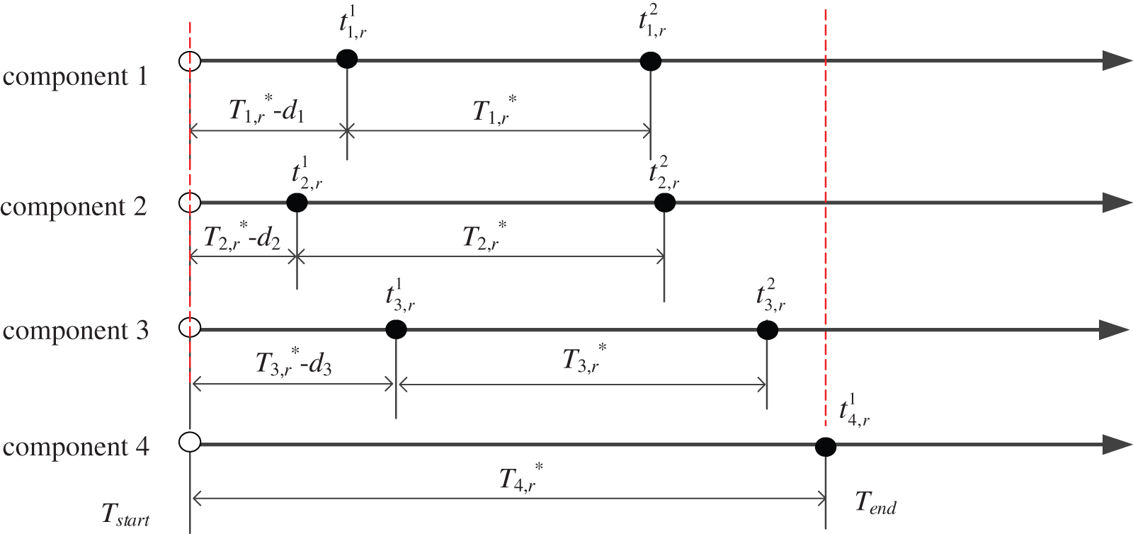
Figure 4: Maintenance activities in planning herizon for a multi-component system with 4 components

Consider grouping n components into N groups. For one of the groups Gk (k=1,…,N), the economic profit is:

EP(Gk)=CSGk−ΔPCGk1(t)+ΔPCGk2(t)(27)

where CSGk is the saving cost caused by grouping; ΔPCGk1∗ represents the penalty cost caused by grouping; and ΔPCGk2∗ denotes the extra profit caused by structure. CSGk is defined as follows:

CSGk=(Lk−1)⋅S(28)

where Lk represents the number of maintenance activities in Gk.

For the penalty cost, the expense of the oth maintenance activity in Ti,r is PCi,r(Δti,ro). According to the definition, PCi,r(Δti,ro) is defined as follows:

PCi,r(Δti,ro)=E[Ci(Ti,r∗+Δti,ro,o)]−E[Ci(Ti,r∗,o)]+Δti,ro⋅Θi,r∗(29)

Then, the penalty cost of all maintenance activities in the maintenance cycles is:

ΔPCGk1(t)=∑LkPCi,r(Δti,ro)(30)

where Δti,ro=t−ti,ro. There is an optimal maintenance time tGk to minimize ΔPCGk1, at which the minimum ΔPCGk1∗ is:

ΔPCGk1∗(t)=mintΔPCGk1∗(tGk)=mint∑LkPCi,r(t−ti,ro)(31)

The additional income ΔPCGk2 is defined as follows:

ΔPCGk2=πGk⋅(CGsum−CGk)(32)

where Gk is the group number and πGk is a critical group indicator function. If Gk contains a critical component, πGk=1; otherwise, πGk=0. Eq. (32) ignores the influence of non-critical components after the failure of some components, so the component importance indicator is introduced into the model, and Eq. (32) is rewritten as:

ΔPCGk2=CIIGk⋅(CGsum−CGk)(33)

where CIIGk is the sum of all component importance indicators in group Gk, and CGsum is the total preventive maintenance and loss cost of all maintenance activities in group Gk during Tr.

CGsum=∑Lk[πi⋅CPMi,r+(1−πi)⋅cip](34)

Then:

CGk=CPMi,r(35)

According to Eqs. (33)–(35), the additional profit is calculated by:

ΔPCGk2=πGk⋅(∑Lk[πi⋅CPMi,r+(1−πi)⋅cip]−CPMi,r)(36)

According to Eqs. (27), (28), (31) and (36), the optimal economic profit of group Gk is calculated by:

EP(Gk)=CSGk−ΔPCGk1∗(t)+ΔPCGk2(t)(37)

The optimal economic profit EP(Gk) is related to the time interval Ti,r∗ of the optimal depreciation cost. When EP(Gk)>0, grouping maintenance is more cost-effective; when EP(Gk)<0, individual maintenance is more cost-effective. Then, the optimal economic profit of the whole system is the sum of the profit of the total groups, as shown in Eq. (38):

EPsum=∑GkEP(Gk)=∑Gk[CSGk−ΔPCGk1∗(t)+ΔPCGk2(t)](38)

We need to find an optimal grouping strategy that maximizes the overall profit of the system as shown in Eq. (39):

PGe∗=argmaxEPsum(PG)(39)

The solution to Eq. (39) is complicated. Considering the optimal group in the partition results of the arbitrary N group, it is a non-deterministic polynomial complete problem (NP-complete problem). The problem cannot obtain a completely accurate analytical solution, it can only obtain an approximate optimal solution. As the number of components n increases, the number of possible groupings will increase rapidly, leading to a dimensional disaster: when the number of components increases, the time to calculate Eq. (39) will increase geometrically. Therefore, a new solution should be considered.

3.3 Optimization of Grouping Models

To solve this combination problem, a genetic algorithm (GA) is used in this section to solve Eq. (39). Engineering optimization problems usually have a large calculation scale, especially NP problems. Therefore, NP problems need to be grouped to save computing resources. A low-level grouping scheme will lead to optimization results that are far from the optimal result. For a grouping of NP problems, the parallel computing feature of a GA can greatly save computing time. The GA concept is an important field in artificial intelligence and operations research. It is a common algorithm for solving NP problems and has been applied in the fields of reliability, risk, safety and maintenance engineering [35]. When dealing with decision-making problems and determining optimal solutions, especially when constraints or multi-criteria are considered, GAs perform well and can significantly reduce the calculation time [36,37]. Consequently, this study uses a genetic algorithm to solve the grouping optimization problem. The GA optimization grouping results are explained in detail in the next paragraph.

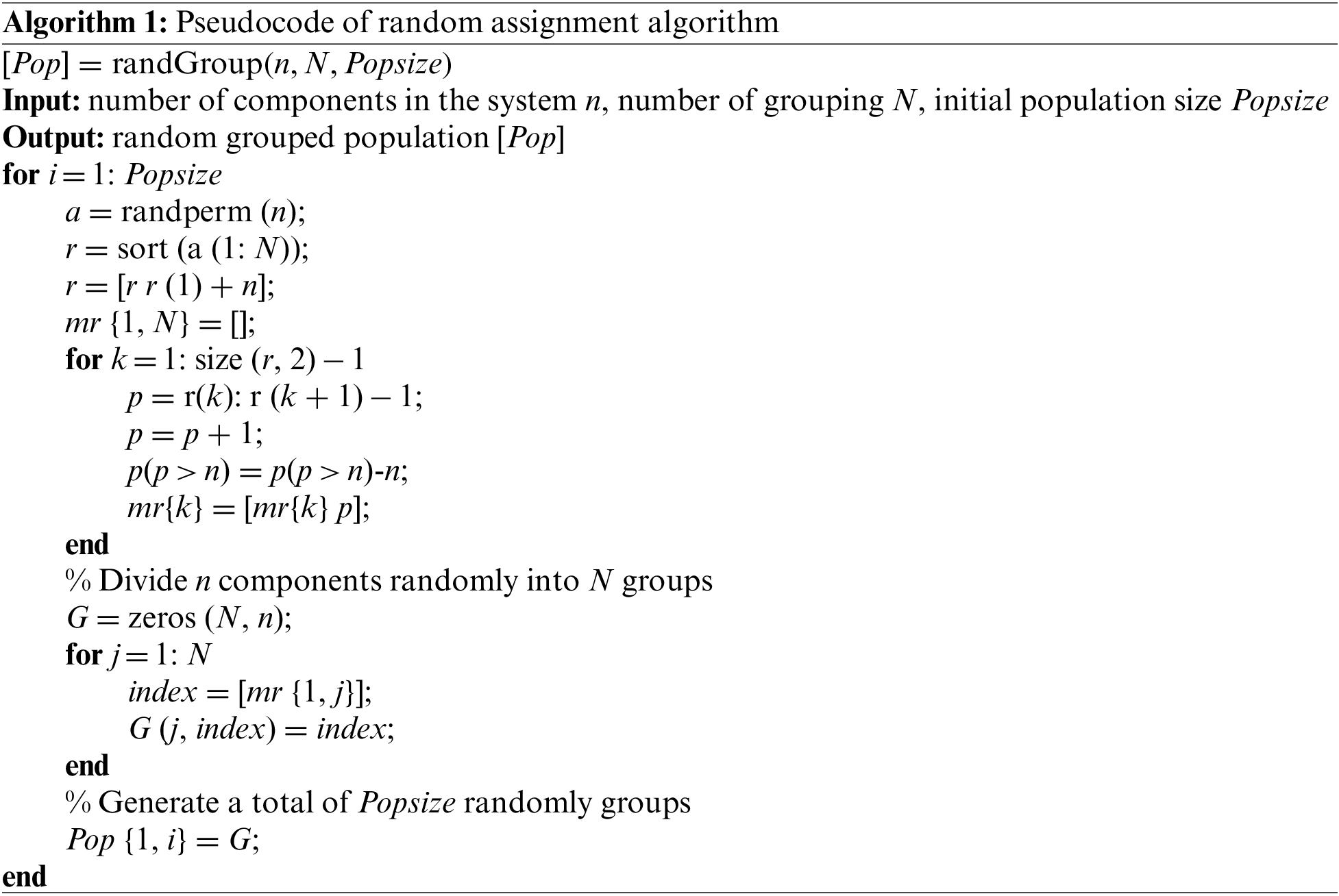
(1)   Initialization

Searching for the optimal solution begins with the generation of the initial population. The methods for initial population generation include random generation and heuristic algorithms, among which the random strategy is the simplest as it has no deviation and does not need initial data.

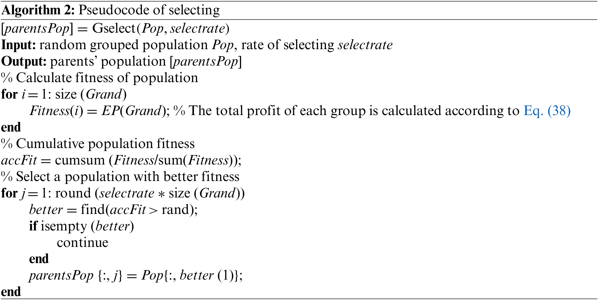
(2)   Selecting

Eq. (38) is a population fitness equation. The selection method is the roulette wheel selection algorithm.

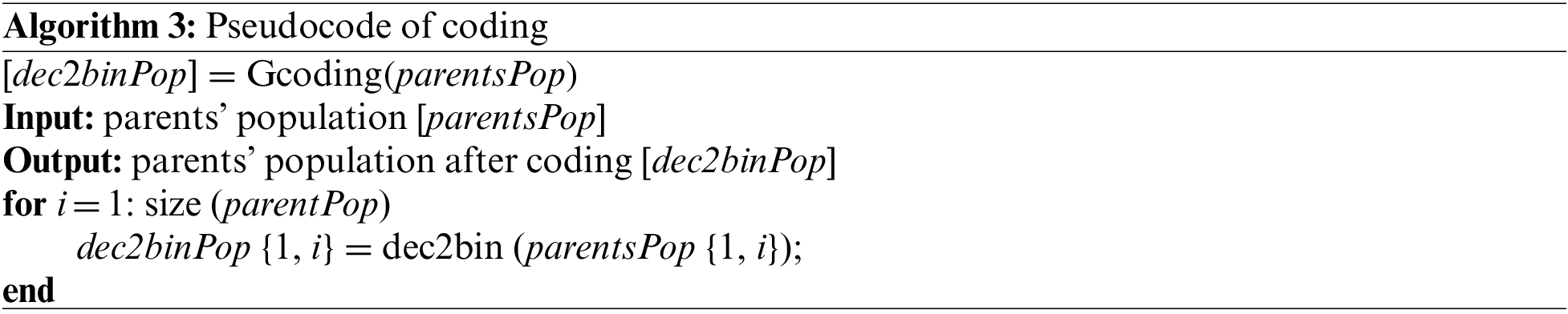
(3)   Coding

The parental population with better fitness is converted into binary code.

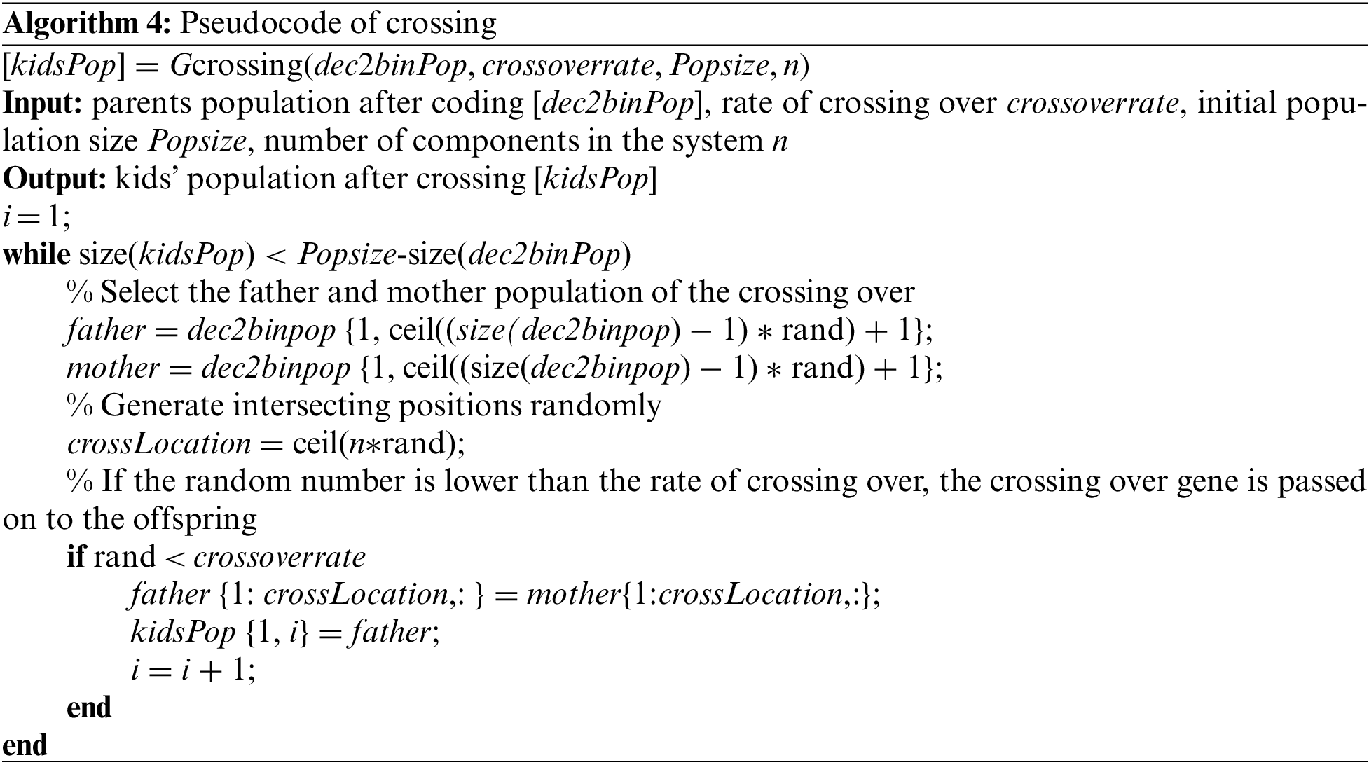
(4)   Crossing

The crossing location is randomly selected in parental generation. The chromosomes of the father population and the mother population interchange after the crossing location. The chromosomes exchanged are passed on to the offspring. The crossing result is shown in Fig. 5 when n = 8 and N = 3. The eight components are randomly divided into three groups and the number 0 is a placeholder, which has no effect on population fitness. The offspring acquires the chromosomes exchanged from the parents.

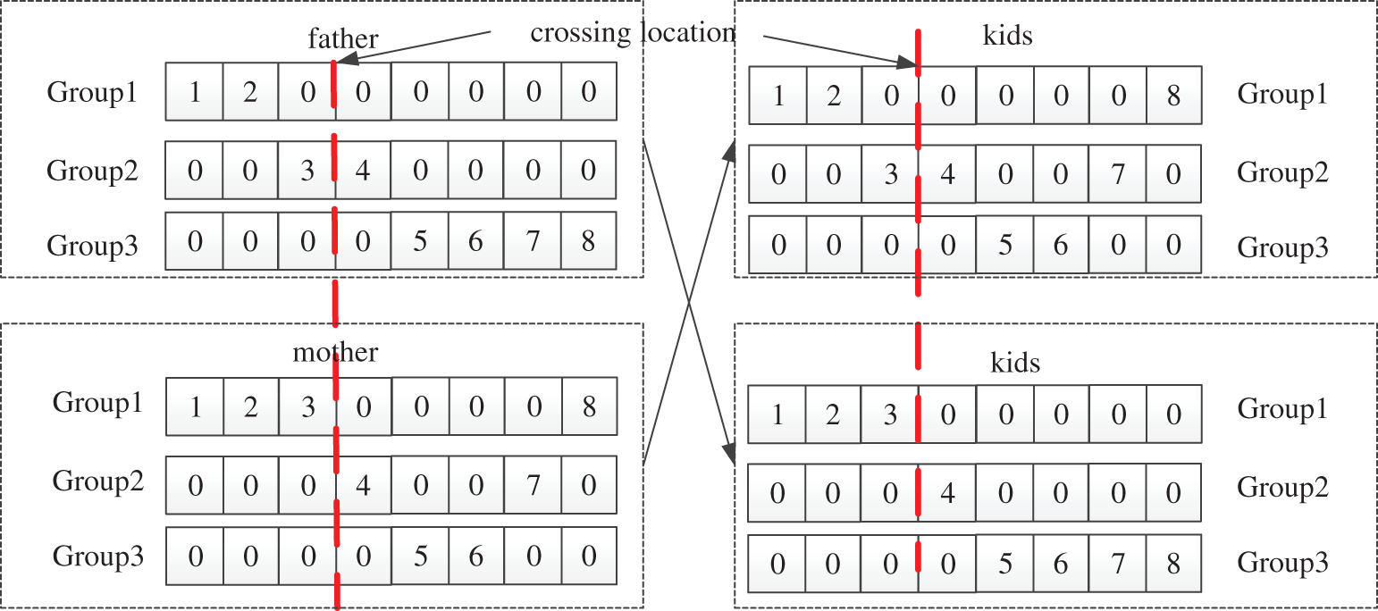
Figure 5: Crossing result

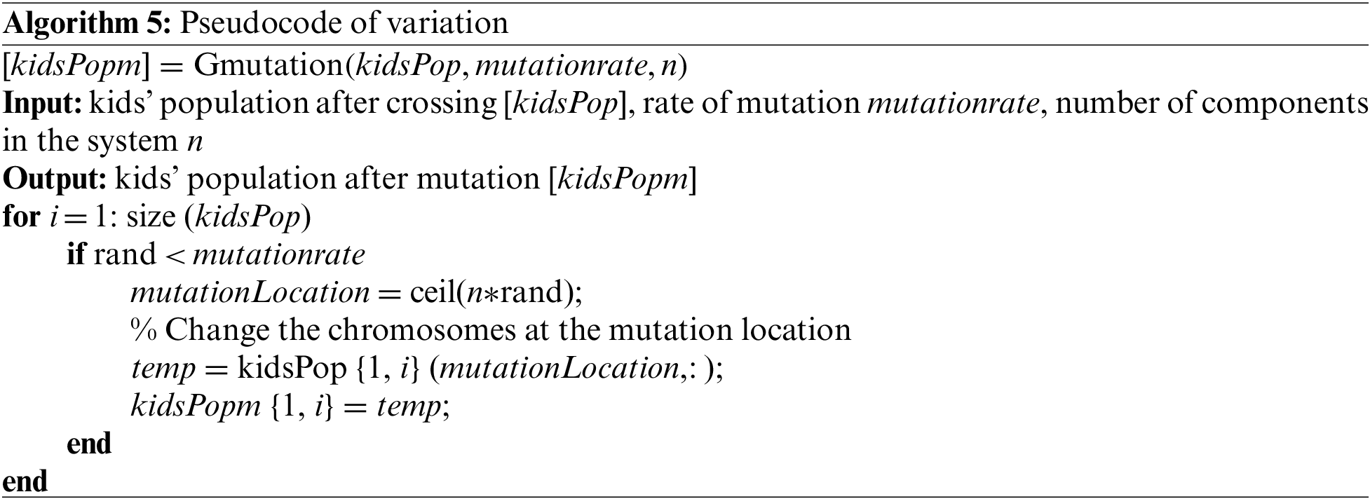
(5)   Mutation

Mutation occurs in the offspring, and the mutation location where the chromosomes change is selected randomly. The mutation result is shown in Fig. 6 when the number of groups n = 8 and N = 3. The grouping of components at the mutation location is changed.

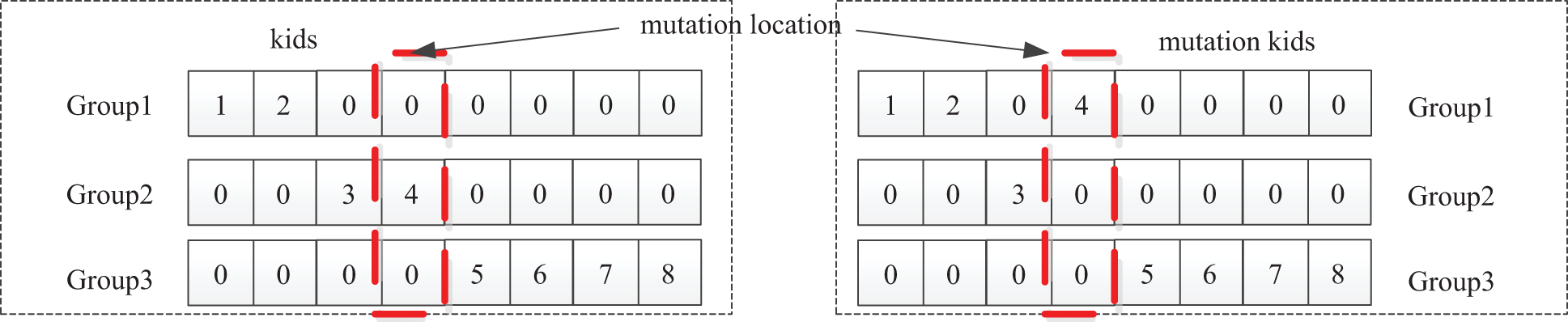
Figure 6: Mutation result

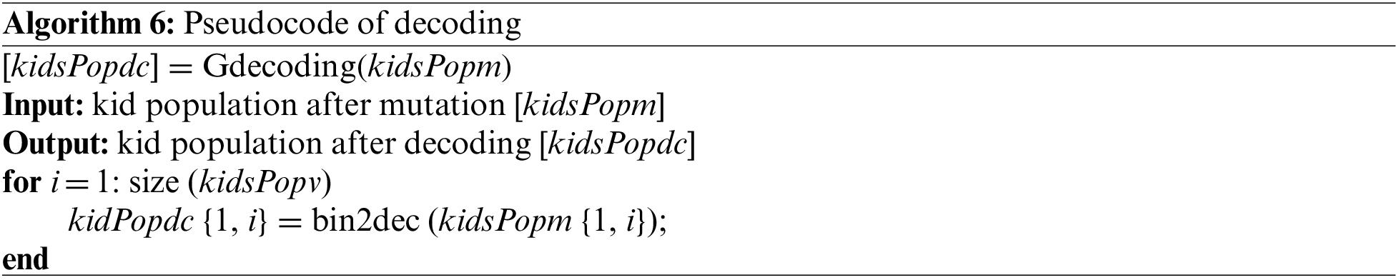
(6)   Decoding

The kids’ population is decoded.

4  Numerical Example

In this section, a gearbox containing 11 components will be used for a numerical simulation to illustrate the feasibility of the proposed grouping maintenance strategy and its importance for multi-component systems. The RBD of the gearbox system is shown in Fig. 7. This is a complex system that includes series, parallel and series–parallel structures, which are universal and widely applicable. This structure is chosen to analyze the influence of system structure on maintenance strategy. In addition, the influence of initial parameters and multiple maintenance cycles on maintenance strategy is also discussed.

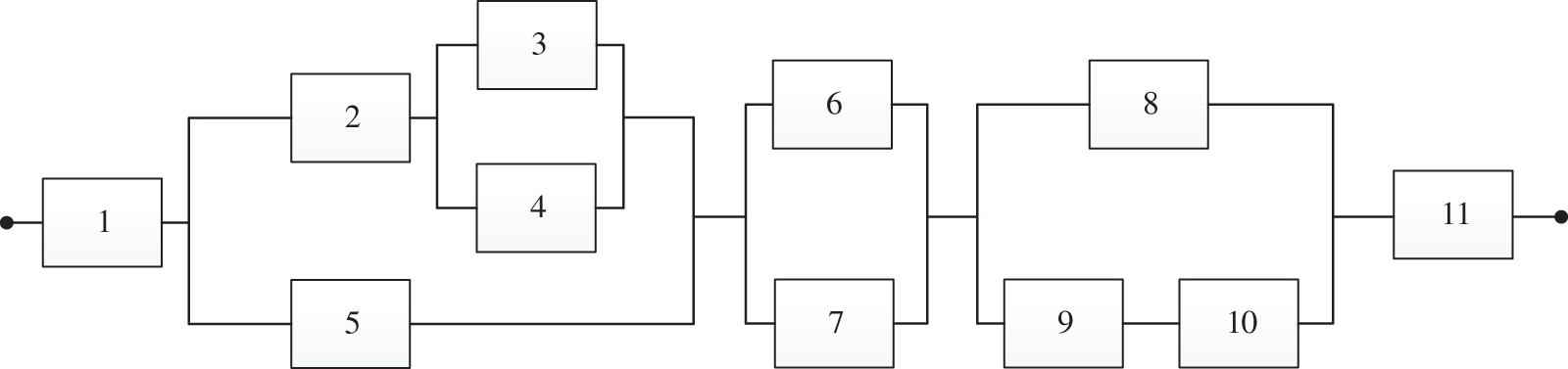
Figure 7: Reliability block diagram of gear case

4.1 Influence of System Structure on Maintenance Policies

This section assumes that the degradation of each component is independent. According to the degradation state of each component in the gearbox, the system reliability parameters are ζ and ψ. Table 2 shows the reliability parameters and the relevant cost parameters of the n = 11 system in the first maintenance cycle. Set the cost of unplanned downtime Cu=40, the preventive downtime cost Cp=30, the penalty cost cip=0, and the labor and preparation cost S=20. The scale of economic cost unit and time cost unit mentioned in the example is scalable, which means that the unit could be arbitrary time or an economic unit.

For the first maintenance cycle, the components in the gearbox are new. Therefore, in the first maintenance cycle, the optimal interval and the minimum average maintenance cost per unit time is simplified as Ti,r∗=(CPMi,r+S)ψi,rζi,r/CFi,r⋅(ζi,r−1)ζi,r and Θi,r∗=(CPMi,r⋅ζi,r)/[Ti,r∗⋅(ζi,r−1)], without considering the depreciation factor j. The parameters of a single component model are then calculated as shown in Table 3.

According to the information in the table, each component is independent when the effect of grouping on the economic profit of the system is not considered. Therefore, each component is a critical component. Setting Tstart=0, according to Eq. (23), we know that Tend=7.74. Therefore, the maintenance cycle is Tr = [0, 7.74]. Then, the average maintenance cost per unit time is Θr=∑Θi,r∗=4679.7, and the maintenance cost within a maintenance cycle is TΘr=Θr∗⋅(Tend−Tstart)=36221.

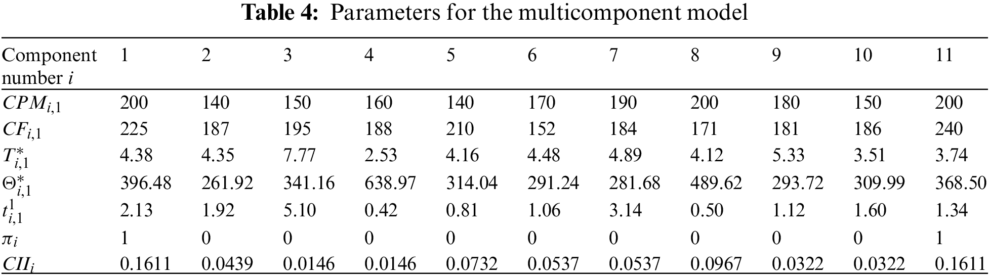
Now consider the effect of structure on the system economic profit. Critical components and related parameters are calculated according to the model in Section 3, as shown in Table 4.

The genetic algorithm is used to calculate the optimal grouping. The initial population size is 100, the number of iterations is 100, the crossing over rate is 0.7, the selection rate is 0.5 and the mutation rate is 0.01. The grouping results are shown in Table 5. The preventive maintenance strategy with one group (PdM-OG) in the table considers all components as a group. The critical component parameters remain the same. PdM-SI is short for preventive maintenance strategy with structural impact; PdM-CII means preventive maintenance strategy with a component importance indicator. The gear box maintenance strategy in the first maintenance cycle is shown in Fig. 8.

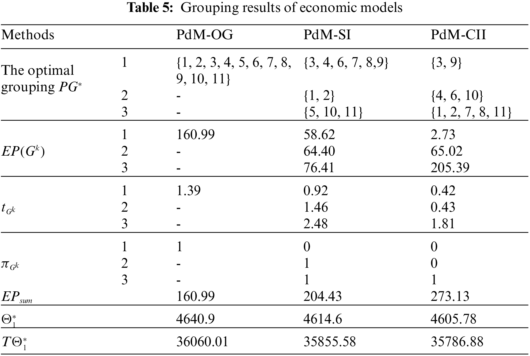
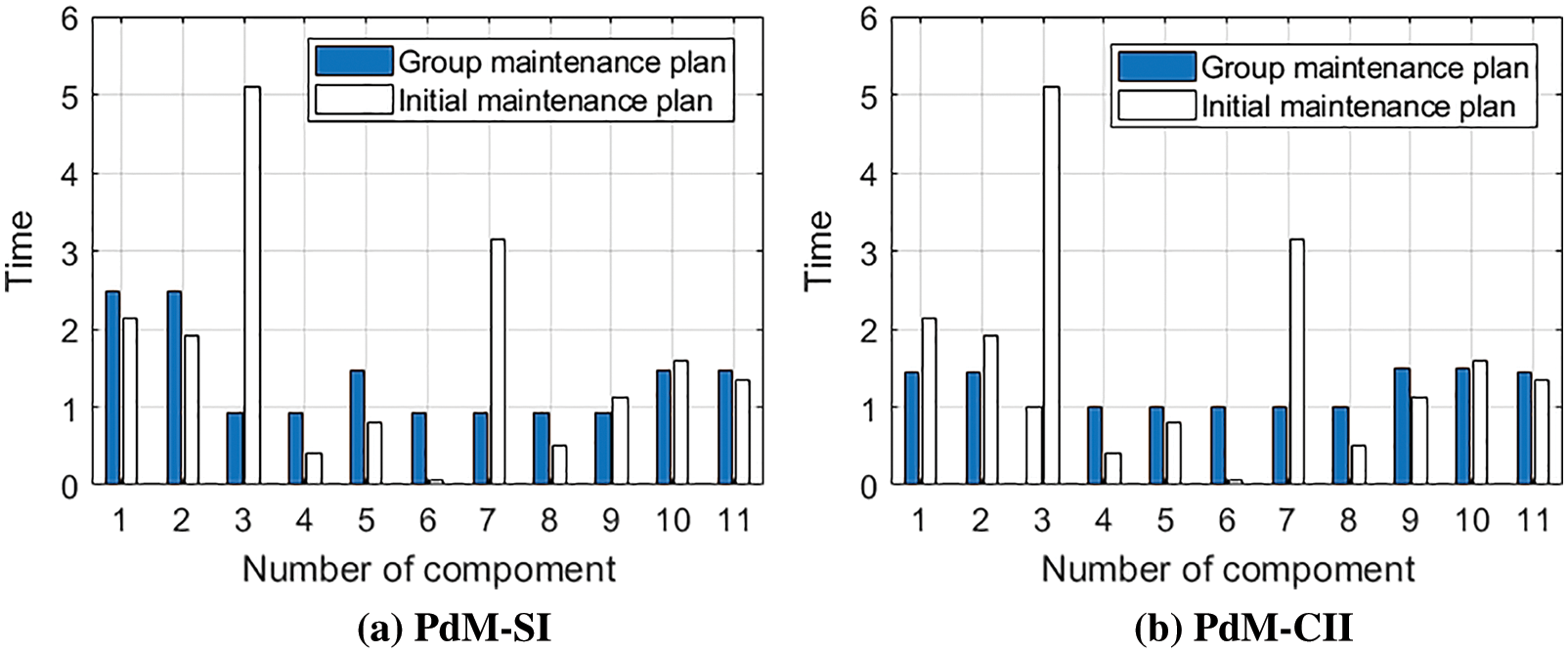
Figure 8: The grouping policy for the first maintenance cycle

In the PDM-OG method, TΘ1∗=36221−160.99=36060.01 and Θ1∗=TΘ1∗/(Tend−Tstart) = 36060.01/(7.77 − 0) = 4640.9. Comparing the maintenance cost of PDM-OG with the maintenance cost of the single component model, grouping can reduce the system maintenance cost. The maintenance cost decreased from 36221 to 36060.01, and the average maintenance cost per unit time decreased from 4679.7 to 4640.9, which means that the system structure has an impact on maintenance strategy and can provide maintenance strategy with lower costs. At the same time, the series–parallel structure of the system should be taken into account when making maintenance plans for the system. In the PdM-SI method, TΘ1∗ = 36060.01 − 204.43 = 35855.58 and Θ1∗= 35855.58/(7.77 − 0) = 4614.6. In the PdM-CII method TΘ1∗ = 36060.01 − 273.13 = 35786.88 and Θ1∗= 35786.88/(7.77 − 0) = 4605.78. The average and total maintenance costs of PDM-SI and PDM-CII are lower than the maintenance costs of the single component model. The proposed method can reduce the maintenance costs of the multi-component system in the maintenance cycle, indicating that the proposed method is effective. In Fig. 8, the blue bar represents the maintenance plan after grouping, and the red bar represents the initial maintenance plan. The vertical axis represents the maintenance interval for each component, and the blue bar with the same maintenance time indicates that they are in the same group. The optimized grouping maintenance plan differs greatly from the initial maintenance plan, and the proposed method can choose discontinuous maintenance activity groups.

4.2 Influence of System Parameters on Maintenance Policies

The effect of initial parameters on optimal grouping and maintenance policies are considered. Initial parameters generally do not change with the maintenance cycle. First, the influence of labor and preparation cost S on the optimization result of the maintenance strategy is considered. When S increases from 0 to 100, the optimal grouping and corresponding economic profit of the gear box are maintained, and the configuration of the other parameters remains the same. The results are shown in Table 6.

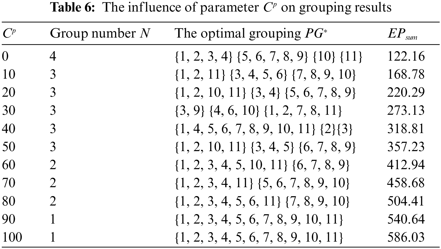
From the table, the economic profit generated by the grouping increases and the total maintenance cost decreases with the increase in S. At the same time, the number of groups N reduces. We then take into consideration the impact of preventive downtime cost Cp on maintenance strategy optimization results. As the cost of preventive shutdown Cp is generally less than the cost of unplanned downtime Cu, we set Cu=Cp+10. When Cp increases from 0 to 100, the optimal grouping and corresponding economic profit of the gear box are maintained, and the configuration of the other parameters remains the same. The results are shown in Table 7. Similar to the influence rule of parameter S, with the increase in preventive downtime cost, the economic profit generated by grouping increases, while the total maintenance cost decreases. Fig. 9 shows the economic profit surface under the influence of S and Cp.

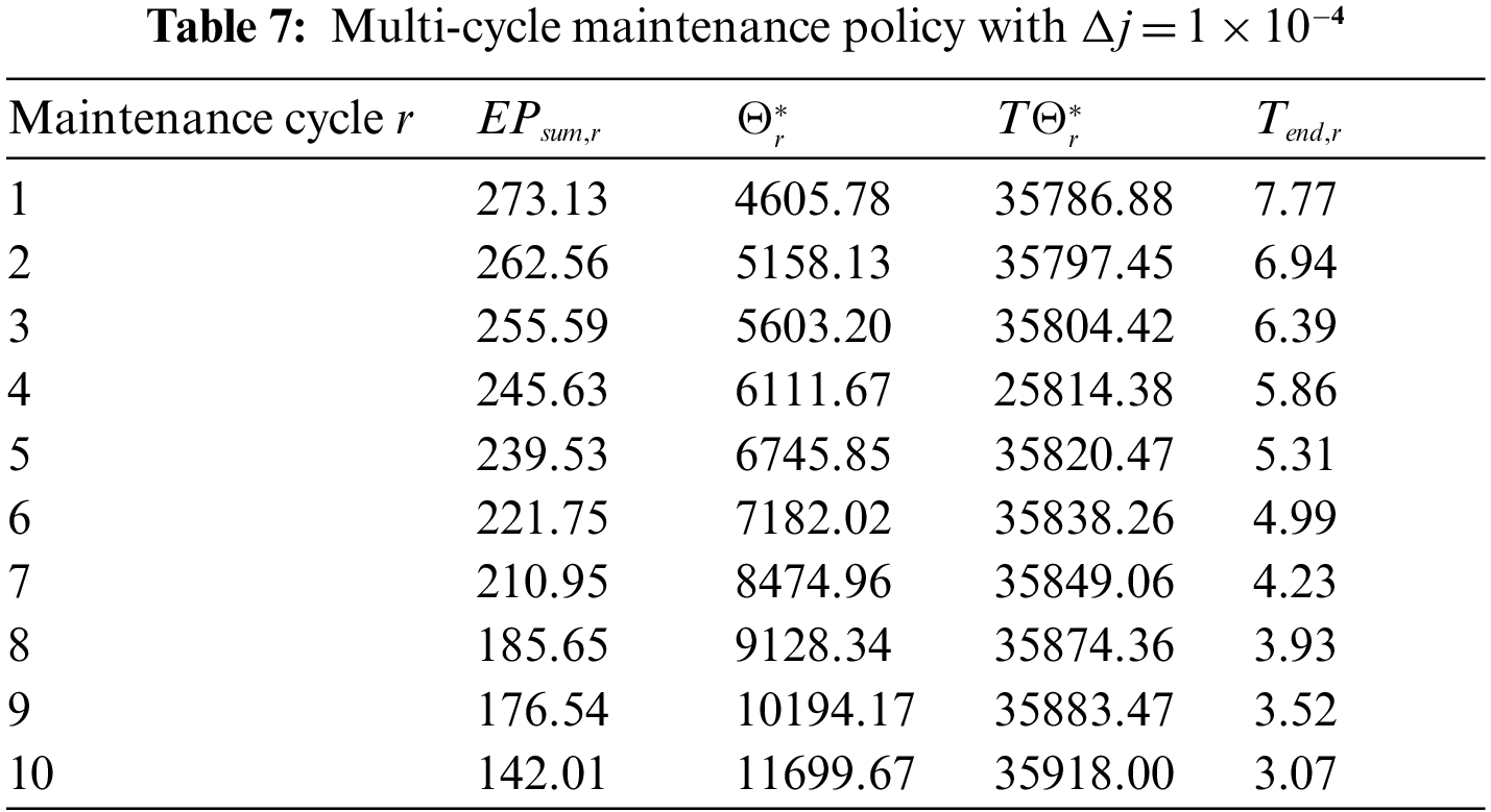
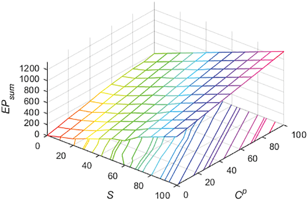
Figure 9: Economic profit surface under common influence S and Cp

The influence of depreciation rate j on the multi-cycle maintenance strategy is considered. In the rth maintenance cycle (r = 1,…, e), the depreciation coefficient varies due to the aging of the equipment, and jr=jr−1−Δj, where Δj is the variation in the depreciation rate within each maintenance cycle. The larger Δj is, the faster the aging rate of the system will be. When the total number of maintenance cycles e = 10, the variation in the depreciation rate coefficient is Δj=1×10−4, Δj=1.7×10−4 and Δj=2.7×10−4, respectively. Tables 8–10 show the maintenance optimization results in multiple maintenance cycles.

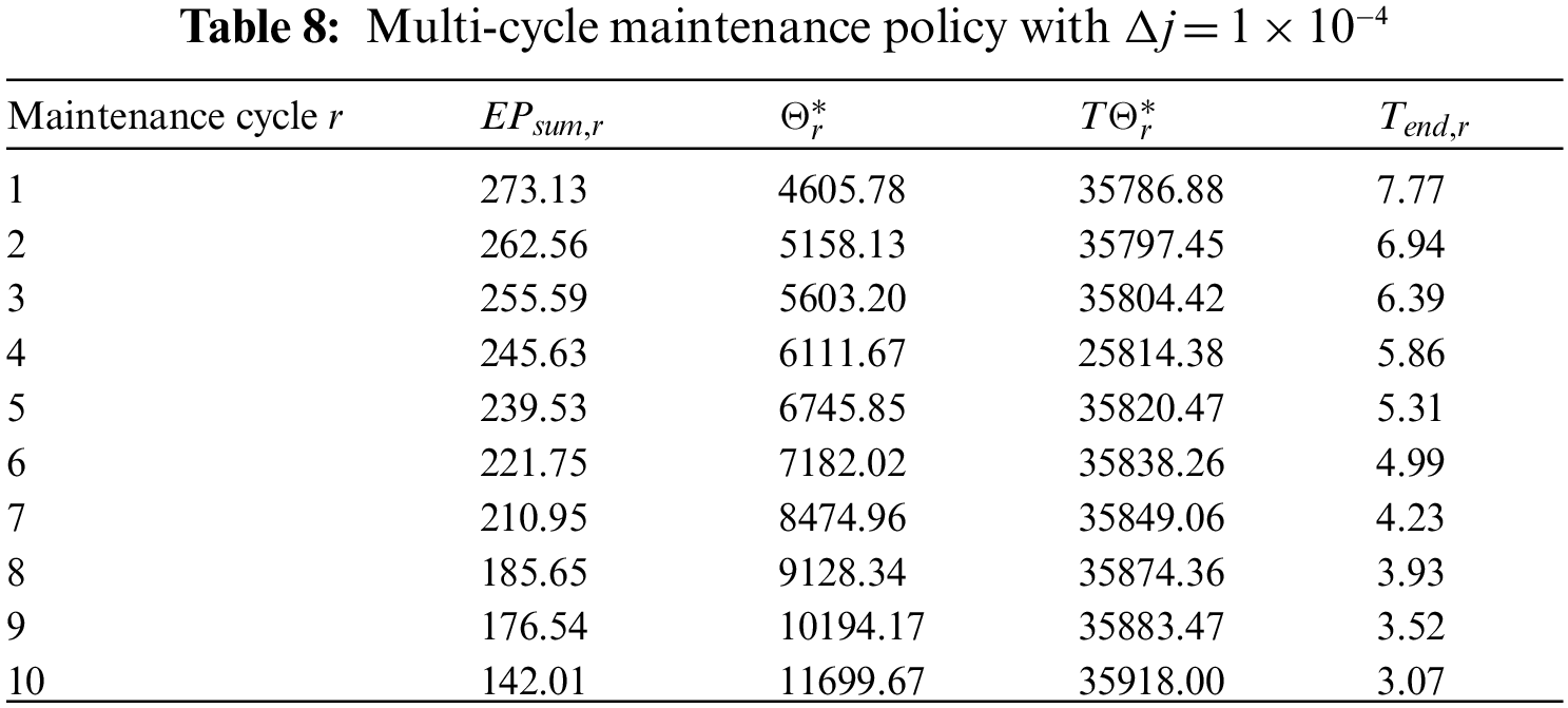
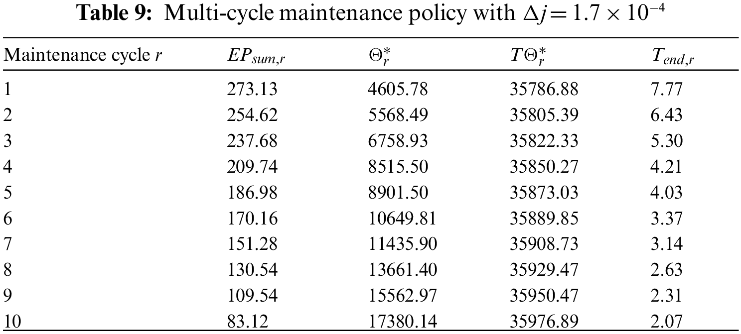
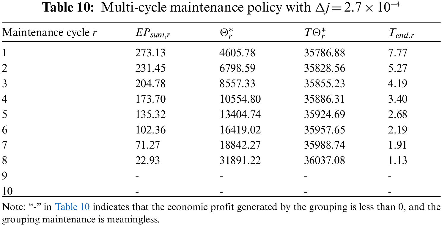
We plot the content in Tables 8–10 as a biaxial diagram, as shown in Fig. 9. The x-axis denotes the cycles of maintenance activities. The y-axis denotes the economic profit of the system EPsum, the minimum average maintenance cost per unit time Θ∗, the end time of maintenance activities Tend and the maintenance cost TΘr∗ in [0,Tend].

As shown in Fig. 10, with the increase in maintenance cycles, the economic profit EPsum caused by system grouping decreases. Meanwhile, the minimum average maintenance cost per unit time Θ∗ of the system increases, and the corresponding maintenance cost TΘr∗ also increases. In addition, the maintenance activities become more frequent. This indicates that wear and tear of the gear box system is constantly occurring with use, and its health condition is gradually degrading, requiring a higher frequency of maintenance activities to ensure its normal operation.

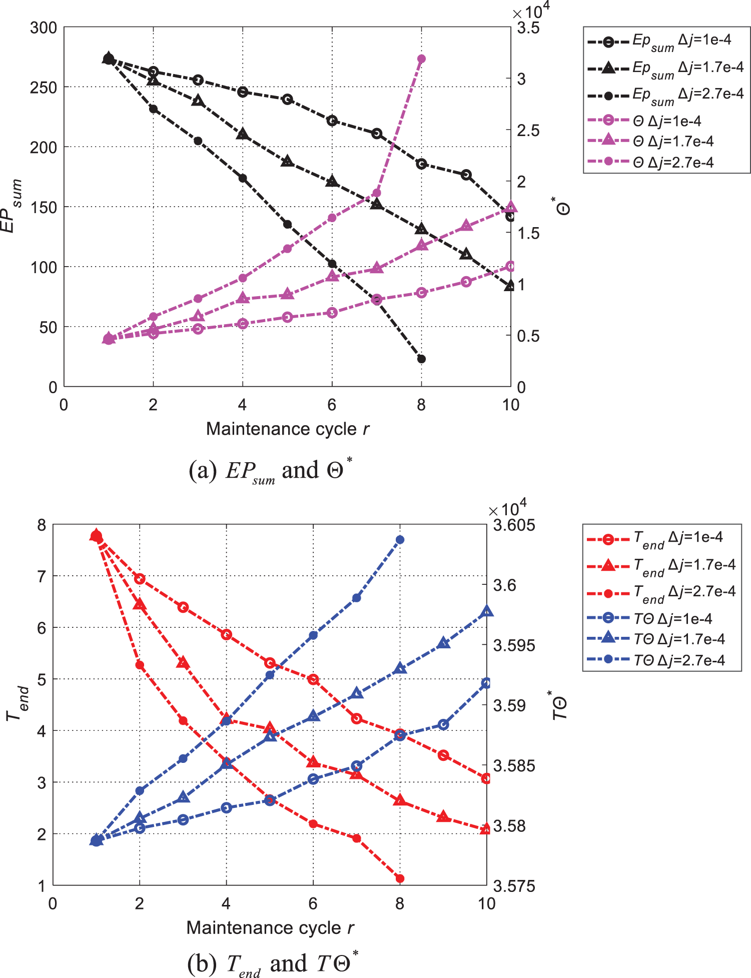
Figure 10: Influence of depreciation coefficient j on results of multiple maintenance cycles

5  Conclusion

This paper proposes a maintenance strategy based on structure dependency. The degradation state of the component is converted to a failure probability model, and the failure probability model of the component in the current degradation state is obtained. The development of preventive maintenance policies for components based on fault probability models is proposed. The main work and conclusions are as follows.

First, a maintenance grouping model that considers system structure is proposed. The grouping model considers the influence of the degree of importance of different components on the system. The results show that the proposed model provides a better expected depreciation cost and economic profit than the maintenance strategy of a model that does not consider the structure.

Second, an optimization model with maintenance cost as the response equation is established. A random grouping scheme based on a genetic algorithm is used to solve the NP problem caused by the multi-component model, and the optimal maintenance time interval is calculated to provide the maintenance strategy.

Third, the influence of the maintenance cycle on the optimization results is studied. The maintenance plan of the previous cycle may no longer be optimal. By using the flexibility of a genetic algorithm, the proposed grouping strategy considers the influence of the dynamic environment and achieves an optimal update of the maintenance plan.

Fourth, an example of an 11-component complex structure system is given to illustrate the effectiveness of the proposed model. (1) By comparing the models before and after grouping, it can be seen that the cost after grouping is lower, indicating that the proposed method can reduce the maintenance cost of a multi-component system in the maintenance cycle. (2) The influence of the initial parameters and the maintenance cycle on maintenance strategy is discussed. Both affect the formulation of a preventive maintenance strategy: with an increase in initial parameters, the number of optimal groups decreases and the economic profit increases. At the same time, the optimal economic response surface under the influence of multiple parameters is obtained. As the maintenance cycle increases, components require shorter maintenance intervals.

Funding Statement: This work was supported by the National Natural Science Foundation of China under Grant No. 12172100. The authors would like to thank them.

Conflicts of Interest: The authors declare that they have no conflicts of interest to report regarding the present study.

References

1. Zhu, S. P., Liao, D., Liu, Q., Correia, J. A. F. O., De, J. A. M. P. (2019). Nonlinear fatigue damage accumulation: Isodamage curve-based model and life prediction aspects. International Journal of Fatigue, 128, 105185. DOI 10.1016/j.ijfatigue.2019.105185. [Google Scholar] [CrossRef]
2. Zhu, S. P., Hao, Y. Z., Correia, J. A. D., Lesiuk, G. (2019). Nonlinear fatigue damage accumulation and life prediction of metals: A comparative study. Fatigue & Fracture of Engineering Materials & Structures, 42(6), 1271–1282. DOI 10.1111/ffe.12937. [Google Scholar] [CrossRef]
3. Meng, D., Li, Y., He, C., Guo, J., Lv, Z. et al. (2021). Multidisciplinary design for structural integrity using a collaborative optimization method based on adaptive surrogate modelling. Materials & Design, 206, 109789. DOI 10.1016/j.matdes.2021.109789. [Google Scholar] [CrossRef]
4. Ramasso, E., Gouriveau, R. (2014). Remaining useful life estimation by classication of predictions based on a neuro-fuzzy system and theory of belief functions. IEEE Transactions on Reliability, 63(2), 555–566. DOI 10.1109/TR.2014.2315912. [Google Scholar] [CrossRef]
5. Khelif, R., Chebel-Morello, B., Malinowski, S., Laajili, E., Fnaiech, F. et al. (2016). Direct remaining useful life estimation based on support vector regression. IEEE Transactions on Industrial Electronics, 64(3), 2276–2285. DOI 10.1109/TIE.2016.2623260. [Google Scholar] [CrossRef]
6. Kaium, S. A., Hossain, S. A., Ali, J. S. (2019). Modal parameter extraction from measured signal by frequency domain decomposition (FDD) technique. International Journal of Structural Integrity, 11(2), 324–337. DOI 10.1108/IJSI-06-2019-0062. [Google Scholar] [CrossRef]
7. Nasir, N. N. M., Singh, S., Abdullah, S., Haris, S. M. (2019). Accelerating the fatigue analysis based on strain signal using Hilbert–Huang transform. International Journal of Structural Integrity, 10(1), 118–132. DOI 10.1108/IJSI-06-2018-0032. [Google Scholar] [CrossRef]
8. Behera, S. K., Parhi, D. R., Das, H. C. (2019). Approach to establish a hybrid intelligent model for crack diagnosis in a fix-hinge beam structure. International Journal of Structural Integrity, 10(2), 208–229. DOI 10.1108/IJSI-05-2018-0029. [Google Scholar] [CrossRef]
9. Meng, D., Xie, T., Wu, P., He, C., Hu, Z. et al. (2021). An uncertainty-based design optimization strategy with random and interval variables for multidisciplinary engineering systems. Structures, 32, 997–1004. DOI 10.1016/j.istruc.2021.03.020. [Google Scholar] [CrossRef]
10. Babich, D., Bastun, V., Dorodnykh, T. (2019). Structural-probabilistic modeling of fatigue failure under elastic-plastic deformation. International Journal of Structural Integrity, 10(4), 484–496. DOI 10.1108/IJSI-05-2018-0024. [Google Scholar] [CrossRef]
11. Meng, D., Yang, S., Lin, T., Wang, J., Yang, H. et al. (2022). RBMDO using Gaussian mixture model-based second-order mean-value saddlepoint approximation. Computer Modeling in Engineering & Sciences, 132(2), 553–568. DOI 10.32604/cmes.2022.020756. [Google Scholar] [CrossRef]
12. Zhu, S. P., Keshtegar, B., Chakraborty, S., Trung, N. T. (2020). Novel probabilistic model for searching most probable point in structural reliability analysis. Computer Methods in Applied Mechanics and Engineering, 366(1), 113027. DOI 10.1016/j.cma.2020.113027. [Google Scholar] [CrossRef]
13. Zhu, S. P., Keshtegar, B., Trung, N. T., Yaseen, Z. M., Bui, D. T. (2021). Reliability-based structural design optimization: Hybridized conjugate mean value approach. Engineering with Computers, 37, 381–394. DOI 10.1007/s00366-019-00829-7. [Google Scholar] [CrossRef]
14. Zhu, S. P., Keshtegar, B., Bagheri, M., Hao, P., Trung, N. T. (2020). Novel hybrid robust method for uncertain reliability analysis using finite conjugate map. Computer Methods in Applied Mechanics and Engineering, 371, 113309. DOI 10.1016/j.cma.2020.113309. [Google Scholar] [CrossRef]
15. Ye, W. L., Zhu, S. P., Niu, X. P., He, J. C., Wang, Q. (2021). Fatigue life prediction of notched components under size effect using stress gradient-based approach. International Journal of Fracture, 234, 249–261. DOI 10.1007/s10704-021-00580-5. [Google Scholar] [CrossRef]
16. Meng, D., Lv, Z., Yang, S., Wang, H., Xie, T. et al. (2021). A time-varying mechanical structure reliability analysis method based on performance degradation. Structures, 34, 3247–3256. DOI 10.1007/s10704-021-00580-5. [Google Scholar] [CrossRef]
17. Tomaru, S., Takahashi, A. (2019). Three-dimensional fatigue crack growth simulation of embedded cracks using s-version FEM. International Journal of Structural Integrity, 11(4), 547–555. DOI 10.1108/IJSI-10-2019-0107. [Google Scholar] [CrossRef]
18. Meng, D., Wang, H., Yang, S., Lv, Z., Hu, Z. et al. (2022). Fault analysis of wind power rolling bearing based on EMD feature extraction. Computer Modeling in Engineering & Sciences, 130(1), 543–558. DOI 10.32604/cmes.2022.018123. [Google Scholar] [CrossRef]
19. Mahdi, M. A., Hussein, A. W. (2019). Investigation the combined effects of wear and turbulent on the performance of hydrodynamic journal bearing operating with couple stress fluids. International Journal of Structural Integrity, 10(6), 825–837. DOI 10.1108/IJSI-11-2018-0083. [Google Scholar] [CrossRef]
20. Meng, D., Yang, S. Q., Zhang, Y., Zhu, S. P. (2019). Structural reliability analysis and uncertainties-based collaborative design and optimization of turbine blades using surrogate model. Fatigue & Fracture of Engineering Materials & Structures, 42(6), 1219–1227. DOI 10.1111/ffe.12906. [Google Scholar] [CrossRef]
21. Susto, G. A., Schirru, A., Pampuri, S., McLoone, S., Beghi, A. (2014). Machine learning for predictive maintenance: A multiple classifier approach. IEEE Transactions on Industrial Informatics, 11(3), 812–820. DOI 10.1109/TII.2014.2349359. [Google Scholar] [CrossRef]
22. Schmidt, B., Wang, L. (2018). Cloud-enhanced predictive maintenance. The International Journal of Advanced Manufacturing Technology, 99(1), 5–13. DOI 10.1007/s00170-016-8983-8. [Google Scholar] [CrossRef]
23. Wei, G., Zhao, X., He, S., He, Z. (2019). Reliability modeling with condition-based maintenance for binary-state deteriorating systems considering zoned shock effects. Computers & Industrial Engineering, 130, 282–297. DOI 10.1016/j.cie.2019.02.034. [Google Scholar] [CrossRef]
24. Zhang, W., Yang, D., Wang, H. (2019). Data-driven methods for predictive maintenance of industrial equipment: A survey. IEEE Systems Journal, 13(3), 2213–2227. DOI 10.1109/JSYST.4267003. [Google Scholar] [CrossRef]
25. Chen, C., Wang, C., Lu, N., Jiang, B., Xing, Y. (2021). A data-driven predictive maintenance strategy based on accurate failure prognostics. Eksploatacja i Niezawodność, 23(2), 387–394. DOI 10.17531/ein.2021.2.19. [Google Scholar] [CrossRef]
26. Theissler, A., Pérez-Velázquez, J., Kettelgerdes, M., Elger, G. (2021). Predictive maintenance enabled by machine learning: Use cases and challenges in the automotive industry. Reliability Engineering & System Safety, 215, 107864. DOI 10.1016/j.ress.2021.107864. [Google Scholar] [CrossRef]
27. Ayvaz, S., Alpay, K. (2021). Predictive maintenance system for production lines in manufacturing: A machine learning approach using IoT data in real-time. Expert Systems with Applications, 173, 114598. DOI 10.1016/j.eswa.2021.114598. [Google Scholar] [CrossRef]
28. Arena, S., Florian, E., Zennaro, I., Orrù, P. F., Sgarbossa, F. (2022). A novel decision support system for managing predictive maintenance strategies based on machine learning approaches. Safety Science, 146, 105529. DOI 10.1016/j.ssci.2021.105529. [Google Scholar] [CrossRef]
29. Do van, P., Barros, A., Bérenguer, C. (2008). Reliability importance analysis of markovian systems at steady state using perturbation analysis. Reliability Engineering & System Safety, 93(11), 1605–1615. DOI 10.1016/j.ress.2008.02.020. [Google Scholar] [CrossRef]
30. Rausand, M., Hoyland, A. (2003). Qualitative system analysis. System reliability theory: Models, statistical methods, and applications. Hoboken, USA: John Wiley & Sons. [Google Scholar]
31. Qiao, H., Tsokos, C. P. (1995). Estimation of the three parameter Weibull probability distribution. Mathematics and Computers in Simulation, 39(1–2), 173–185. DOI 10.1016/0378-4754(95)95213-5. [Google Scholar] [CrossRef]
32. Rinne, H. (2008). The weibull distribution: A handbook, pp. 30. New York: Chapman and Hall/CRC. [Google Scholar]
33. Do van, P., Barros, A., Bérenguer, C., Bouvard, K., Brissaud, F. (2013). Dynamic grouping maintenance with time limited opportunities. Reliability Engineering & System Safety, 120, 51–59. DOI 10.1016/j.ress.2013.03.016. [Google Scholar] [CrossRef]
34. Dasgupta, A., Pecht, M. (1991). Material failure mechanisms and damage models. IEEE Transactions on Reliability, 40(5), 531–536. DOI 10.1109/24.106769. [Google Scholar] [CrossRef]
35. García-Martínez, C., Rodriguez, F. J., Lozano, M. (2018). Genetic algorithms. In: Handbook of heuristics. Cham: Springer. [Google Scholar]
36. Demo, N., Tezzele, M., Rozza, G. (2021). A supervised learning approach involving active subspaces for an efficient genetic algorithm in high-dimensional optimization problems. SIAM Journal on Scientific Computing, 43(3), B831–B853. DOI 10.1137/20M1345219. [Google Scholar] [CrossRef]
37. Kim, H., Kim, P. (2017). Reliability–redundancy allocation problem considering optimal redundancy strategy using parallel genetic algorithm. Reliability Engineering & System Safety, 159, 153–160. DOI 10.1016/j.ress.2016.10.033. [Google Scholar] [CrossRef]
Cite This Article
Copyright © 2023 The Author(s). Published by Tech Science Press.
This work is licensed under a Creative Commons Attribution 4.0 International License , which permits unrestricted use, distribution, and reproduction in any medium, provided the original work is properly cited.
Downloads
Citation Tools