Nonlinear Electrical Impedance Tomography Method Using a Complete Electrode Model for the Characterization of Heterogeneous Domains

1  Introduction

Electrical impedance tomography (EIT) is a nondestructive evaluation method that infers the electrical conductivity, permittivity, or impedance of structures using the surficial measurement of electrical responses due to currents. The method seeks to construct a tomographic image of an object by estimating the spatial distribution of its impedance or electrical conductivity. EIT has been recognized as a highly applicable technique in medical imaging, industrial process monitoring, and near-surface site characterization due to its ease of field experimentation, economic feasibility, and superior ability to penetrate structures. When a structure experiences electric potential difference, current flows from the point of high potential to the point of low potential. In other words, when the electric current is input to a structure, electric potential distribution is formed within the structure and on its boundary. If a structure is heterogeneous, the path of electric current is different from the homogeneous case. Therefore, the electric potential distribution of a structure depends on its material heterogeneity [1,2].

The problem of reconstructing the material properties of a structure using the measured electrical response from the surface can be defined as an inverse medium problem. Many mathematical algorithms and numerical strategies have been proposed to improve the solution to this problem. For example, mathematical and statistical regularization methods have been proposed to relieve the ill-posedness of the inverse problem and improve the solution convergence [3–6]. Representative methods for solving the nonlinear EIT problem include the back-projection method [7], one-step Newton method [8], D-bar method [9], and block method [10]. Recent studies have also investigated combining the EIT technique with neural networks to improve the accuracy of the tomographic image reconstruction of structures [11]. Such developments have been primarily applied to medical imaging for cancer detection and brain activity imaging. In civil engineering, research on the feasibility of applying the EIT to structural condition assessment or site characterization has been increasing recently. Recent applications of the EIT to civil structures include crack detection in pipes buried in the ground [12], ground saturation monitoring, and damage detection in carbon fiber-reinforced polymer (CFRP) materials [13]. To successfully implement the EIT, it is essential to have an efficient and accurate forward solver. In civil engineering applications, however, ensuring the accuracy of the forward solution remains a challenge because of the wide range of material properties, scales, and contact impedance between electrodes and structures.

For improving the previous development of the EIT for civil structures, this study proposes a nonlinear inversion method using a complete electrode model (CEM), targeting the reconstruction of the electrical conductivity profile of heterogeneous domains. The CEM comprises the Laplace equation for electric potential and the boundary conditions that express the current input to the structure via surface electrodes [14–16]. Because the CEM enables the realistic modeling of the interface between the structure and electrodes, accurate solutions of the electric potential in the structural medium and the electrodes are expected. The forward solution generated by the CEM is used within the nonlinear inversion framework for reconstructing the electrical conductivity profile of structures. Specifically, the inverse problem is resolved using a partial differential equation (PDE)-constrained optimization approach. This approach seeks the optimal solution of the medium’s electrical conductivity to minimize a Lagrangian, which comprises a least-squares objective functional augmented by the weak imposition of the governing PDE and boundary conditions from the CEM. Enforcing the stationarity of the Lagrangian leads to state, adjoint, and control problems, which constitute the Karush-Kuhn-Tucker (KKT) optimality conditions. They are the first-order optimality conditions resulting from the first variation of the Lagrangian with respect to state, adjoint, and control variables. The electrical conductivity profile of the domain is then iteratively updated by solving the KKT conditions in the reduced space of the control variable. A conjugate gradient method with an inexact line search is used for the iterative solution of the electrical conductivity. To the best of the authors’ knowledge, the EIT method based on the PDE-constrained optimization using the CEM and KKT conditions has been presented for the first time. The proposed inverse EIT problem deals with the Laplace equation, Robin, and Neumann boundary conditions in the PDE-constrained optimization. There are similar EIT approaches developed so far, but they mostly deal with Neumann or Dirichlet boundary conditions to solve the forward problem [17–19]. Some recent studies have included the Robin boundary condition to reflect the contact impedance between the domain and electrode boundaries, but their inverse formulation and optimization schemes are different from the present study [20,21].

The remainder of this paper is organized as follows: In Section 2, the forward problem described by the CEM is presented. In Section 3, the formulation of the electrostatic inverse medium problem is presented using the Lagrangian functional and the first-order optimality conditions. In Section 4, the inversion process used to iteratively update the electrical conductivity profile in the reduced space is described. Section 5 discusses numerical examples for a series of cases in which homogeneous and heterogeneous electrical conductivity profiles are reconstructed. Finally, Section 6 presents the conclusions of the study. Finite differences for a non-unifrom grid are well shown in Figs. A1–A3.

2  Forward Problem

2.1 Problem Statement Using the Complete Electrode Model

To solve the inverse medium problem using measured electric potential values, it is first necessary to resolve the electrostatic forward problem for calculating the electric potential due to the current input. This study uses the CEM as a mathematical model for the forward problem. The CEM accounts for the current loss that occurs when the current flows to a low impedance material through an electrode and the voltage drops due to the contact impedance between the structural surface and electrode [14,22]. The current loss and voltage drop influence the measured electric potential values detected by the electrodes. As the CEM considers both the contact impedance and current loss at the electrodes, the error between the calculated electric potential and the experimentally derived electric potential is generally smaller than that computed using other models. Fig. 1 schematically shows a circular structure with electrodes on its surface. Solving the forward problem using the CEM reveals the electric potential inside the structure and that at the electrodes due to the current input through the electrodes.

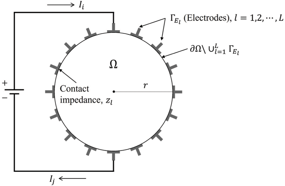
Figure 1: Schematic of a circular structure and surface electrodes

The forward problem described by the CEM can be formulated as the following boundary value problem:

∇⋅(σ∇u)=0,x∈Ω,(1)

u+zlσ∂u∂n=Ul,l=1,2,…,L,x∈ΓEl,(2a)

∫ΓElσ∂u∂ndΓ=Il,l=1,2,…,L,x∈ΓEl,(2b)

σ∂u∂n=0,x∈∂Ω∖∪l=1LΓEl,(2c)

where Ω denotes the structural domain, u is the scalar electric potential, σ is the electrical conductivity, n is the outward unit normal on the boundary ∂Ω, El denotes the lth electrode, ΓEl is the lth electrode boundary, zl is the contact impedance of El, Il is the injected current at El, Ul is the electric potential at El, and L is the number of electrodes. To ensure the existence and uniqueness of solutions, we add

∑l=1LIl=0,(3)

to the model. To determine the reference point for the electric potential,

∑l=1LUl=0(4)

must be satisfied. We multiply Eq. (1) by a test function v(x) and integrate it over the domain Ω, which results in

∫∂Ωvσ∂u∂nd∂Ω−∫Ω∇v⋅(σ∇u)dΩ=0.(5)

Using the boundary conditions (2a) and (2c), Eq. (5) can be rewritten as

∑l=1L1zl∫ΓElv(Ul−u)dΓ−∫Ω∇v⋅(σ∇u)dΩ=0.(6)

Next, we integrate Eq. (2a) over ΓEl, which results in

∫ΓEludΓ=∫ΓEl(Ul−zlσ∂u∂n)dΓ=Ul|el|−zlIl.(7)

Eq. (7) is multiplied by a test value Vl, divided by zl, and summed for all electrodes, which yields

∑l=1L1zlVl(∫ΓEludΓ−Ul|el|+zlIl)=0.(8)

Adding Eqs. (6) and (8) results in

∑l=1L1zl[∫ΓElv(Ul−u)dΓ+Vl(∫ΓEl(u−Ul)dΓ+zlIl)]−∫Ωσ∇v⋅∇udΩ=0,→∑l=1L1zl[∫ΓElv(Ul−u)dΓ+Vl(∫ΓEl(u−Ul)dΓ)]+∑l=1LIlVl−∫Ωσ∇v⋅∇udΩ=0,→∫Ωσ∇u⋅∇vdΩ+∑l=1L1zl∫ΓEl(u−Ul)(v−Vl)dΓ=∑l=1LIlVl.(9)

Eq. (9) is the weak form of the forward problem. The electric potential u in the domain and the potential U at the electrodes are approximated using Legendre basis functions ϕi(x) and basis vectors nj, respectively:

u(x)≅uh(x)=∑j=1Nαjϕj(x),(10)

U≅Uh=∑j=1L−1βjnj,(11)

where N is the number of nodes in the finite element mesh. The coefficient αj is the nodal value of u(x), βj is the unknown parameter for linearly combining vectors nj, and Uh is a vector consisting of the electric potential at each electrode. The basis vectors nj∈RL×1 are defined as

n1=[1−100⋮0],n2=[10−10⋮0],n3=[100−1⋮0],…,nL−1=[1000⋮−1].(12)

The choice of nj ensures that Eq. (4) is satisfied. The test function v and the value of Vl at the electrode can be similarly approximated as

vh(x)=∑i=1Nviϕi(x),(13)

Vh=∑i=1L−1Vini,(14)

where Vh is a vector consisting of the value of V at each electrode. By substituting Eqs. (10), (11), (13), and (14) into the weak form represented by Eq. (9), a linear system of equations for unknown vector u=[αTβT]T can be obtained

Ku=F;[BCCTD][αβ]=[0I],(15)

where the matrices and vectors are written as

Bij=∫Ωσ∇ϕi⋅∇ϕjdΩ+∑l=1L1zl∫ΓElϕiϕjdΓ(1≤i≤N)(1≤j≤N),(16a)

Cij=−(1z1∫ΓE1ϕidΓ−1zj+1∫ΓEj+1ϕidΓ)(1≤i≤N)(1≤j≤L−1),(16b)

CijT=Cji=−(1z1∫ΓE1ϕjdΓ−1zi+1∫ΓEi+1ϕjdΓ)(1≤i≤L−1)(1≤j≤N),(16c)

Dij={|e1|z1,i≠j|e1|z1−|ej+1|zj+1,i=j(1≤i≤L−1)(1≤j≤L−1),(16d)

0∈RN×1,I=[I1−I2I1−I3I1−I4⋮I1−IL]∈R(L−1)×1,(17)

α=[α1α2α3⋮αN]∈RN×1,β=[β1β2β3⋮βL−1]∈R(L−1)×1.(18)

In Eq. (16d), |el| is the length of the lth electrode. Solving Eq. (15) yields nodal values of the electric potential in the domain as well as the values of β. The potentials Ulh at the electrodes can be obtained as follows:

Ulh=[U1hU2hU3h⋮ULh]=[∑l=1L−1βl−β1−β2⋮−βL−1].(19)

2.2 Validation of Forward Solutions

For validation, the forward solutions are compared to the solutions obtained using Technology Computer-Aided Design (TCAD) software. TCAD is used for modeling electronic design processes and the behavior of electrical devices based on fundamental physics [23]. Fig. 2 shows the configuration of a circular domain with a radius of 10 cm. The electrical conductivity of the domain is 1.56×10−1S/cm. A total of 16 electrodes is arranged to cover 50% of the boundary; a current of 0.78 A is input into the fifth electrode, and it flows out through the 13th electrode. The contact impedance of the electrodes is 9.8×10−7Ω⋅cm2. In this case, the potential of the fifth electrode is 10 V. Fig. 3 shows the distribution of the calculated electric potential within the domain due to the current input. The numerical solution calculated using the CEM is very close to the result obtained using the TCAD software.

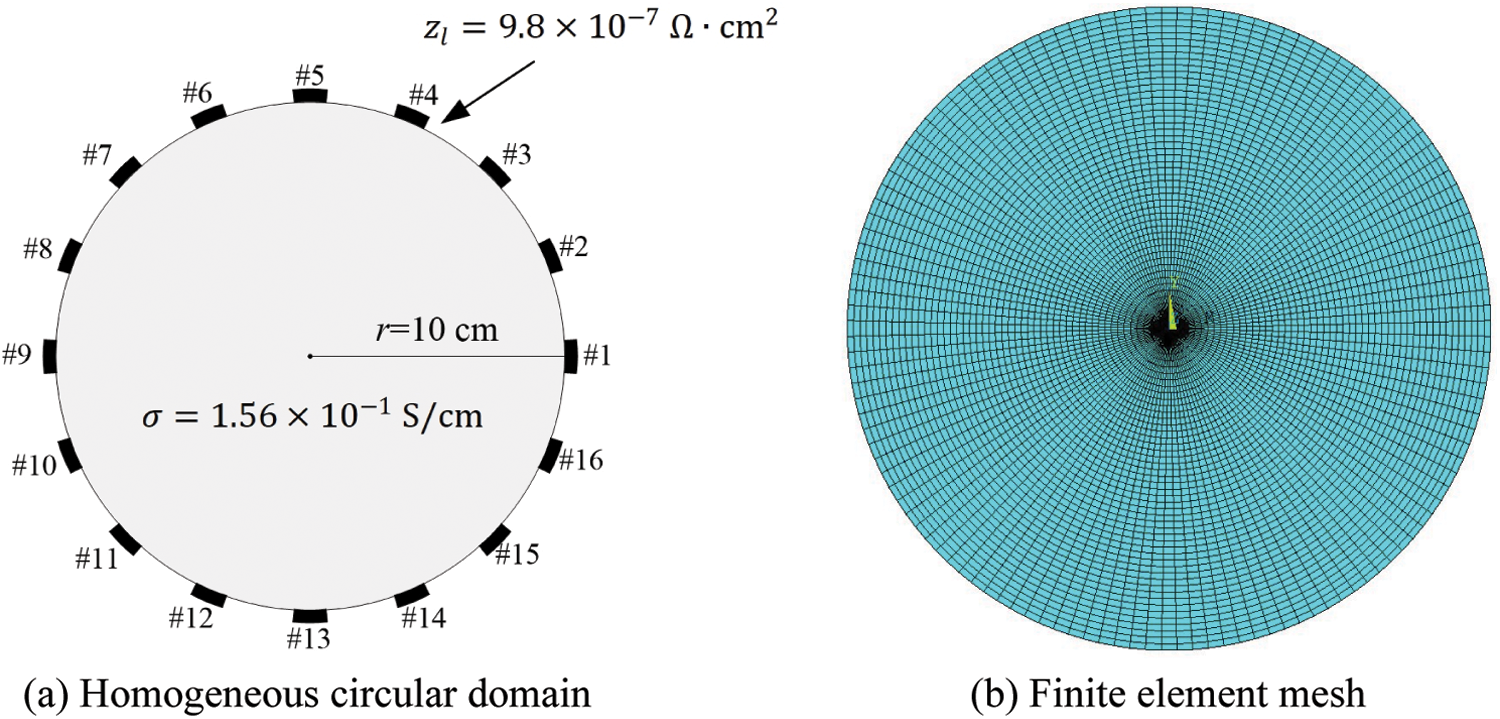
Figure 2: Homogeneous circular domain and finite element mesh for validating the forward solution

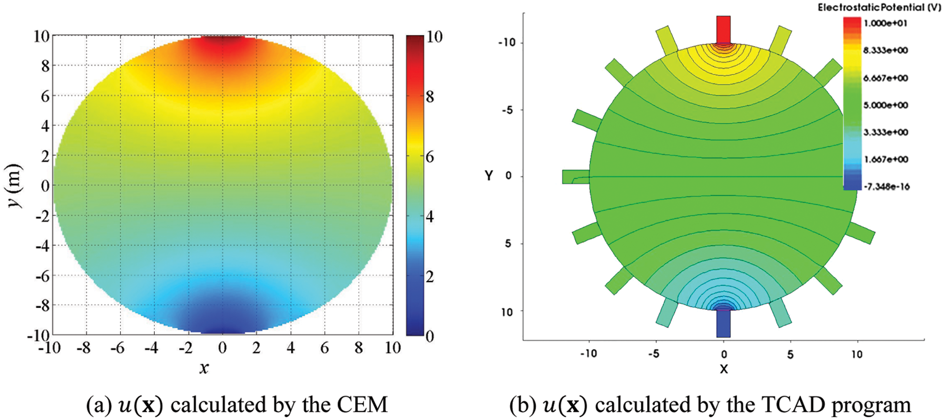
Figure 3: Calculated electric potential, u(x), in the homogeneous circular domain

The error of the forward solution relative to the TCAD result can be calculated using the following equation:

Error (%)=|VCEM−VTCAD|VTCAD×100.(20)

Table 1 shows the electric potential values at each electrode and the corresponding relative errors. The maximum error is 3.37%, which demonstrates the accuracy of the forward solution. Fig. 4 depicts the electric potential, Ul, calculated at each electrode.

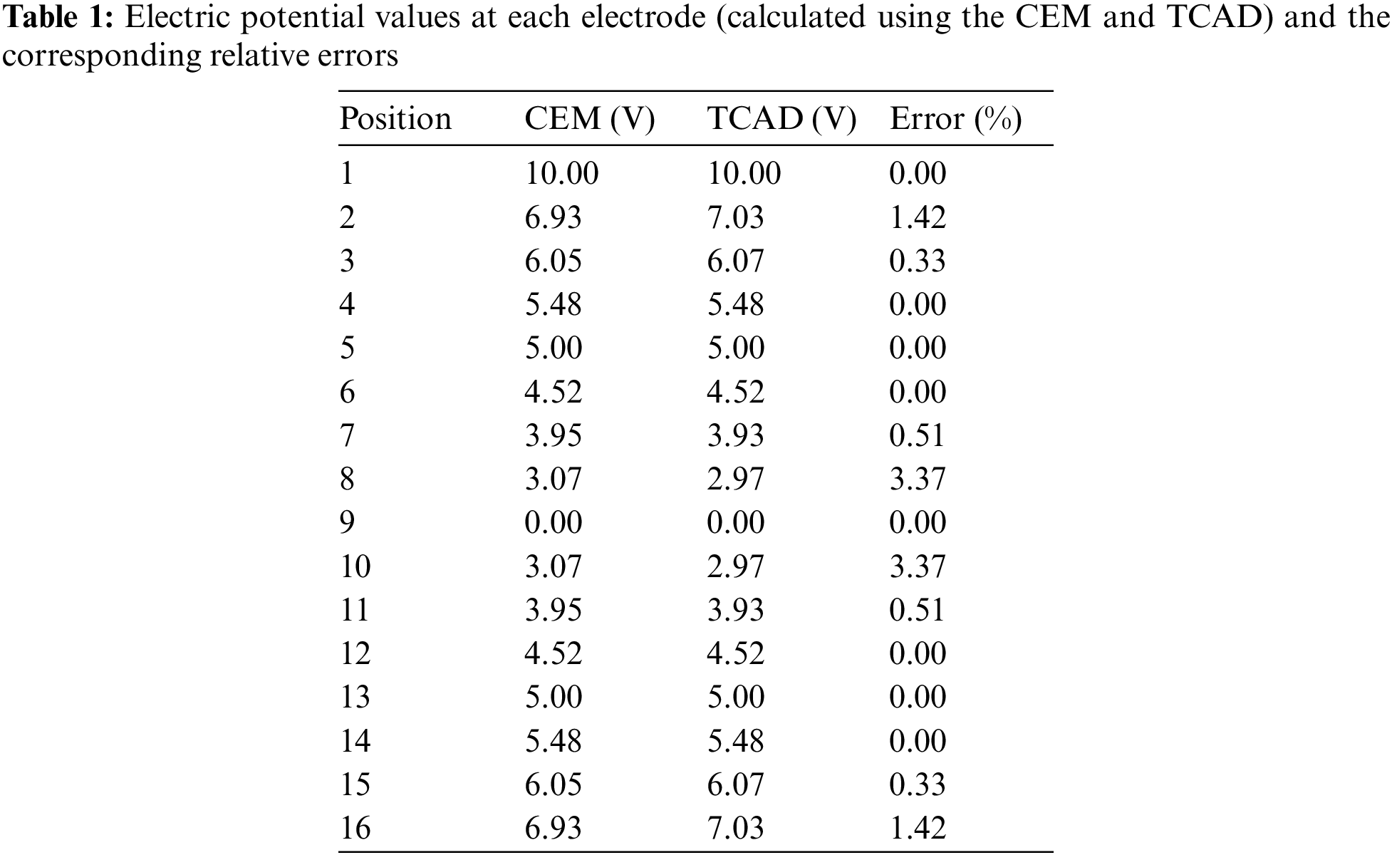
Figure 4: Graphical representation of the electrical potential at each electrode

2.3 Mesh-Type Dependency of the Forward Solution

For investigating the dependency of the forward solutions on the finite element mesh, two mesh types are explored: a radial mesh composed of eight-node quadrilateral elements and a mixed mesh with a square section inside. Fig. 5 illustrates these two types of meshes.

Figure 5: Two finite element mesh types for forward and inverse analyses

Fig. 6 shows a circular domain with a radius of 15 cm and electrodes attached to its boundary. The domain is assumed to be homogeneous, with an electrical conductivity of 1×10−2S/cm, which is typical of concrete materials. A total of 32 electrodes is arranged on the boundary and are spaced evenly to cover 50% of the boundary (as for the domain described in Section 2.2). A current with a cosine pattern along the perimeter is input to each electrode. The magnitude of the current at each electrode is Il=cos⁡(2πl/L), where L is the total number of electrodes, and l is the index for the electrode number. The contact impedance of the electrodes is 0.22Ω⋅cm2. Fig. 7 presents the forward solutions calculated using the two meshes displayed in Fig. 5. Fig. 7c shows the calculated electric potential values at the electrodes on the boundary. The two results show that the forward solution changes minimally with the mesh type.

Figure 6: Homogeneous circular domain with 32 electrodes on the boundary

Figure 7: Forward solutions calculated using the two meshes

3  Inverse Problem

3.1 PDE-Constrained Optimization

The problem of reconstructing the electrical conductivity profile of a structure using the electric potential measured at surface electrodes can be formulated as the following PDE-constrained optimization problem:

minσ(x)J:=12∑l=1L∫ΓEl(Ul−Ulm)2dΓ+γ(σ).(21)

The objective functional J consists of a misfit functional in a least-squares sense and a regularization term γ(σ). The misfit functional is expressed as the sum of the squared differences between the calculated electric potential Ul and the measured electric potential Ulm at electrode El. This optimization problem is constrained by the governing Eq. (1) and boundary conditions (2)–(4) of the forward problem. To relieve the ill-posedness of the inverse problem, the regularization term γ(σ) is included in the objective functional J. In this study, the Tikhonov (TN) regularization scheme is used; thus, the regularization term can be written as

γ(σ)=12Rσ∫Ω∇σ⋅∇σdΩ,(22)

where Rσ is a regularization factor that controls the penalty to the gradient of the electrical conductivity σ(x). Although TN regularization cannot accurately capture sharply varying material profiles, it still assists the inversion process in narrowing the feasibility space of solutions and improving the solution convergence.

3.2 First-Order Optimality Conditions

The PDE-constrained optimization problem can be converted to an unconstrained optimization problem using a Lagrange multiplier method. Specifically, the objective functional J can be augmented by Eqs. (1) and (2b) to construct the Lagrangian functional L,

L(u,Ul,w,Wl,σ)=12∑l=1L∫ΓEl(Ul−Ulm)2dΓ+γ(σ)+∫Ωw∇⋅(σ∇u)dΩ+∑l=1L∫ΓElWl(σ∂u∂n−Il)dΓ,(23)

where w and Wl are Lagrange multipliers applied to the left-hand terms of the governing equation and boundary conditions, respectively. The electrical conductivity σ(x) that minimizes the Lagrangian is the solution to the inverse problem. For the optimal solutions, first-order optimality conditions are introduced, which enforce the first variation of the Lagrangian with respect to state variables u and Ul, adjoint variables w and Wl, and the control variable σ to vanish.

3.2.1 First Optimality Condition: State Problem

At the optimum of the Lagrangian, its first variation with respect to the adjoint variables w and Wl should vanish. Introducing the stationarity conditions δwL=0,δWlL=0, and l=1,2,…L results in the state problem, which is identical to the forward problem presented in Eqs. (1) and (2).

3.2.2 Second Optimality Condition: Adjoint Problem

At the optimum of the Lagrangian, its first variation with respect to the state variables u and Ul should vanish as well. Applying the stationarity requirements, δuL=0,δUlL=0, and l=1,2,…L, to the Lagrangian yields

δuL+∑l=1LδUlL=∑l=1L∫ΓlδUl(Ul−Ulm−σ∂w∂n)dΓ+∫Ωδu∇⋅(σ∇w)dΩ−∫Γfδuσ∂w∂ndΓf+∑l=1L∫Γl∂δu∂nσ(w+zlσ∂w∂n+Wl)dΓ=0.(24)

Because δu and δUl(l=1,2,…L) are arbitrary, Eq. (24) results in the following adjoint problem:

∇⋅(σ∇w)=0,x∈Ω,(25)

w+zlσ∂w∂n=−Wl,l=1,2,…,L,x∈ΓEl,(26a)

σ∂w∂n=Ul−Ulm,l=1,2,…,L,x∈ΓEl,(26b)

σ∂w∂n=0.x∈∂Ω∖∪l=1LΓEl,(26c)

Eq. (25) is the governing equation for adjoint variable w(x), and Eqs. (26a)–(26c) are boundary conditions for w(x) and Wl. Eq. (26b) indicates the source of the adjoint problem, which depends on the potential misfit at the electrodes. The adjoint problem has the same differential operators as the state problem does.

3.2.3 Third Optimality Condition: Control Problem

Finally, the first variation of the Lagrangian with respect to the control variable σ should vanish at the optimum. Introducing the stationarity condition (δσL=0) to the Lagrangian results in

δσL=Rσ∫Ωδσ(−RσΔσ−∇w⋅∇u)dΩ+∑l=1L∫Γlδσ(Rσ∂σ∂n+w∂u∂n+Wl∂u∂n)dΓ+∫Γfδσ(Rσ∂σ∂n+w∂u∂n)dΓ=0.(27)

Because δσ is arbitary, Eq. (27) yields the following control problem:

−RσΔσ−∇w⋅∇u=0,x∈Ω,(28)

Rσ∂σ∂n+w∂u∂n+Wl∂u∂n=0,l=1,2,…,L,x∈ΓEl,(29a)

Rσ∂σ∂n+w∂u∂n=0.x∈∂Ω∖∪l=1LΓEl(29b)

The control problem is a boundary value problem for the electrical conductivity σ(x), with Eq. (28) being the governing equation and Eqs. (29a) and (29b) being the boundary conditions. The solution σ(x) can be calculated once the state and adjoint solutions u, w, and Wl are obtained. The state, adjoint, and control problems constitute the KKT conditions for the PDE-constrained optimization problem.

4  Inversion Setup and the Simulation Process

4.1 Finite Element Formulation of the Adjoint Problem

The adjoint problem described in Section 3.2.2 can be solved using the Galerkin finite element method. Specifically, Eq. (25) is multiplied by a test function v(x) and integrated over the entire domain Ω. Upon integrating the resulting equation by parts and using a procedure similar to that represented by Eqs. (5) to (9), the weak form of the adjoint problem can be derived as

∫Ωσ∇w⋅∇vdΩ+∑l=1L1zl∫ΓEl(w−Wl)(v−Vl)dΓ=∑l=1L(Ul−Ulm)Vl|el|,(30)

where Vl is a test value used to derive the weak form of Eq. (26a). The adjoint solutions w and Wl can be approximated using Legendre basis functions ϕi(x) and basis vectors nj, respectively, as follows:

w(x)≅wh(x)=∑j=1Nαjadjϕj(x),(31)

W≅Wh=∑j=1L−1βjadjnj,(32)

where αjadj is the nodal value of w(x), βjadj is the unknown parameter for linearly combining vectors nj, and Wh is a vector consisting of Wl at each electrode. The test functions v and Vl are approximated using Eqs. (13) and (14).

Substituting Eqs. (13), (14), (31) and (32) into (30) results in the following linear system of equations:

Kadjuadj=Fadj;[BadjCadj(−Cadj)TDadj][αadjβadj]=[0Iadj],(33)

where Kadj, uadj, and Fadj are the stiffness matrix, solution vector, and right-hand side vector of the adjoint problem, respectively. The superscript “adj” denotes the adjoint problem. The matrices and vectors in Eq. (33) can be written as

Bijadj=∫Ωσ∇ϕi⋅∇ϕjdΩ+∑l=1L1zl∫ΓElϕiϕjdΓ,(1≤i≤N)(1≤j≤N)(34a)

Cijadj=1z1∫ΓE1ϕidΓ−1zj+1∫ΓEj+1ϕidΓ,(1≤i≤N)(1≤j≤L−1)(34b)

(−Cijadj)T=−Cjiadj=−(1z1∫ΓE1ϕjdΓ−1zi+1∫ΓEi+1ϕjdΓ),(1≤i≤L−1)(1≤j≤N)(34c)

Dijadj={−|e1|z1,i≠j−|e1|z1−|ej+1|zj+1,i=j(1≤i≤L−1)(1≤j≤L−1),(34d)

0∈RN×1,Iadj=[(U1−U1m)|e1|−(U2−U2m)|e2|(U1−U1m)|e1|−(U3−U3m)|e3|(U1−U1m)|e1|−(U4−U4m)|e4|⋮(U1−U1m)|e1|−(UL−ULm)|eL|]∈R(L−1)×1,(35)

αadj=[α1adjα2adjα3adj⋮αNadj]∈RN×1,βadj=[β1adjβ2adjβ3adj⋮βL−1adj]∈R(L−1)×1.(36)

Solving Eq. (33) yields nodal values of adjoint variable w in the domain as well as the values of βadj. The adjoint variable Wlh at the electrodes can be derived as

Wlh=[W1hW2hW3h⋮WLh]=[∑l=1L−1βladj−β1adj−β2adj⋮−βL−1adj].(37)

The submatrices in Eq. (33) are related to those of the state problem through

Badj=B,(38a)

Cadj=−C,(38b)

(−Cadj)T=CT,(38c)

Dadj=−D.(38d)

Eq. (38) contributes to reducing the computational cost of constructing the system matrices of the adjoint problem in the inversion process.

4.2 Material Property Update

By solving the state and adjoint problems, the first and second optimality conditions are satisfied. Only the true profile of σ(x) exactly satisfies the control problem represented by Eqs. (28) and (29). Therefore, the material profile σ(x) must be updated to satisfy the third optimality condition. Updating σ(x) to minimize the Lagrangian L requires a reduced gradient for L. The process of updating the control variable σ(x) using the state and adjoint solutions can be summarized as follows:

1) Assuming the initial profile of σ(x), solve the forward problem (1) and (2) for state variables u(x) and Ul.

2) Using the state solution Ul, solve the adjoint problem (25) and (26) for adjoint solutions w(x) and Wl.

3) Using the state and adjoint solutions, calculate the reduced gradient for L with respect to the control variable σ(x) as

gσ≡∇σL=−RσΔσ−∇w⋅∇u=−Rσ(∂2σ∂x2+∂2σ∂y2)+(−∂w∂x∂u∂x−∂w∂y∂u∂y),(39)

where the derivatives are calculated using second-order accurate finite difference methods. When using a radial mesh, such as that shown in Fig. 5a, the reduced gradient (40) expressed in a cylindrical coordinate system can be used

gσ=−Rσ(∂2σ∂r2+1r∂σ∂r+1r2∂2σ∂θ2)+(−∂w∂r∂u∂r−1r2∂w∂θ∂u∂θ).(40)

4) Determine the search direction using a line search method and update the electrical conductivity profile σ(x).

4.2.1 Conjugate Gradient Method with Inexact Line Search

In this study, the search direction for the optimal solution of the control variable σ is determined using the Fle´tcher-Reeves conjugate gradient method with an inexact line search. The continuous form of the reduced gradient, Eqs. (39) or (40), can be discretized by being evaluated at each nodal point. Let gk denote the discrete reduced gradient at the kth inversion iteration,

gk=(∇σL)k.(41)

Then, the electrical conductivity vector σk comprising nodal values of σ is updated via

σk+1=σk+αdk,(42)

where dk is a search direction vector at σk, and α is the step length in the direction of dk. By using the Fle´tcher-Reeves method, the search direction vector is calculated as

dk={−gk,k=0,−gk+gk⋅gkgk−1⋅gk−1dk−1,k≥1.(43)

The misfit functional is evaluated using the updated electrical conductivity σk+1 and is compared to a preset tolerance. If it does not meet the tolerance criterion, the inversion process set k←k+1 and proceeded to the next iteration. As is known, the discrete search direction vector dk gradually deviates from the direction to a local minimum because of the non-optimal step length α and the round-off error arising from the accumulation of the gk⋅gk/gk−1⋅gk−1 terms in Eq. (43). Therefore, it is necessary to reset dm+1 to −gm+1 after every mth iteration.

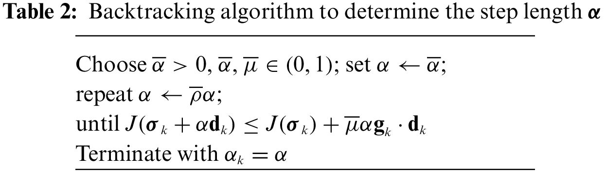
In this study, an inexact line search method is used to determine a step length α that would yield an adequate reduction in the objective functional J. Specifically, the method requires the step length to reduce the objective functional sufficiently, as indicated by the Armijo condition (or sufficient decrease condition); this condition is expressed as

J(σk+αdk)≤J(σk)+μ¯αgk⋅dk,(44)

where μ¯ is selected to be a small value, which is μ¯=10−10 in this study. To satisfy the Armijo condition, the backtracking algorithm described in Table 2 can be used. In this procedure, an initial step length α¯ is set at the beginning. If Eq. (44) is violated during the inversion, the step length is iteratively reduced by setting α←ρ¯α. In this study, ρ¯=0.5 is used.

4.2.2 Regularization Factor Continuation Scheme

The choice of the regularization factor Rσ in Eqs. (39) or (40) considerably affects the reconstruction of the electrical conductivity profile. If Rσ is excessively large, it may be difficult to capture a sharply varying interface in the profile because of the large penalty on the gradient of σ(x). Conversely, if Rσ is excessively small, the inversion may suffer from a solution multiplicity problem. To determine the optimal regularization factor at each inversion iteration, a regularization factor continuation scheme [24–26] is used in this study. The reduced gradient in Eqs. (39) or (40) can be formally rewritten as

∇σL=Rσ(∇σJr)+∇σJm,(45)

in which

∇σJr=−Δσ,(46a)

∇σJm=−∇w⋅∇u.(46b)

In Eq. (45), Rσ(∇σJr) represents the gradient of the regularization functional, and ∇σJm denotes the gradient of the misfit functional. The first term, Rσ(∇σJr), penalizes spatial oscillations in the inverted profile such that an increasing Rσ results in a smoother inverted profile. A balance between these two terms can be imposed using

Rσ|∇σJr|<|∇σJm|⟹Rσ<|∇σJm||∇σJr|.(47)

Therefore, Rσ can be calculated at each iteration as

Rσ=ε|∇σJm||∇σJr|,(0≤ε≤1),(48)

where the value of the weight factor ε is between 0.5 and 1, as recommended for a reasonable regularization effect.

5  Numerical Results

5.1 Homogeneous Domains

Consider a circular domain with a radius of 15 cm, as shown in Fig. 8. A total of 32 electrodes is placed on the boundary and spaced evenly to cover 50% of the boundary. For finite element implementation, the mixed mesh illustrated in Fig. 5b is used. The contact impedance of the electrodes is 0.22Ω⋅cm2. The initial value of the regularization factor Rσ is 1.0, and the weight factor ε for the regularization factor continuation scheme is 0.5. As an excitation to the domain, a current with a cosine pattern, as expressed in Eq. (49), is input to each electrode along the circular perimeter,

Figure 8: Schematic of a circular domain and 32 surface electrodes used for inversion

Il=cos⁡(2πl/32),l=1,2,…,32.(49)

Fig. 9 shows the target, initial guess, and reconstructed electrical conductivity profiles. The target profile is homogeneous with σtg=1.0 S/cm, which is typical of graphite materials. The inversion starts with an initial guess of σini=0.5 S/cm and reconstructs the target profile accurately at about 700 iterations. Fig. 9d shows the response misfit as a function of the iteration number during the inversion process. The misfit decreases from 3×102 to 1.49×10−3, which represents a reduction on the order of 10−5. The response misfit, Fm, as part of the objective functional J in Eq. (21), can be written as

Figure 9: Numerical inversion for homogeneous target profile

Fm=12∑l=1L∫ΓEl(Ul−Ulm)2dΓ.(50)

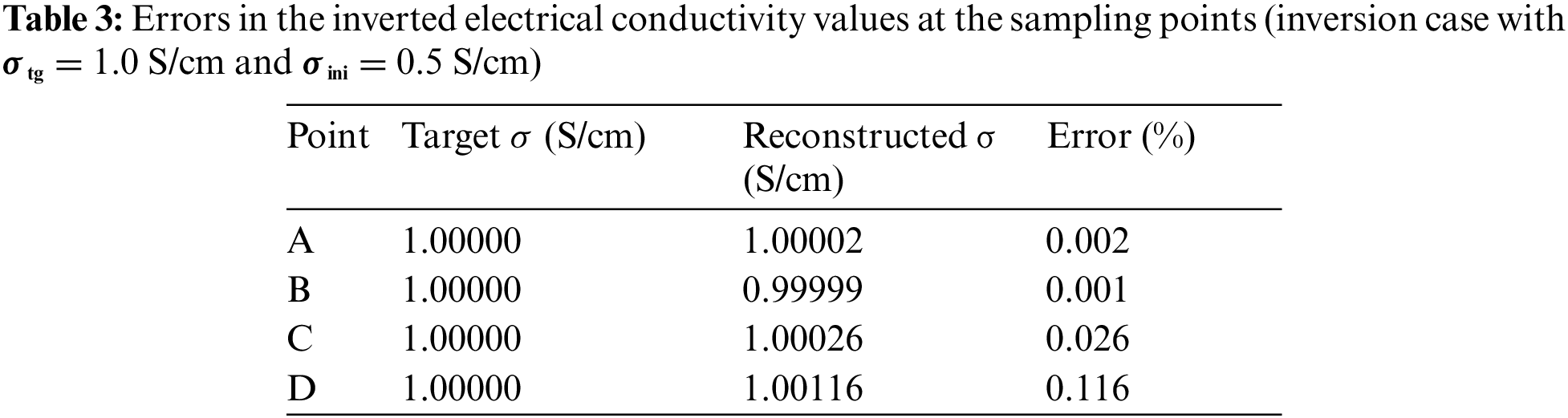
To investigate the accuracy of the inversion result, the errors in the inverted electrical conductivity values are calculated at four sampling points, as shown in Fig. 10: A(0,0), B(4,0), C(8,0), and D(12,0). Table 3 lists the errors at each sampling point. The maximum error is 0.116%, which demonstrates that the inversion for the homogeneous electrical conductivity profile is highly accurate.

Figure 10: Sampling points for error calculation

To investigate the effect of the initial guess on the reconstructed profile, four cases of the inversion with different initial-to-target ratios are considered. Table 4 shows the four cases for the initial guess σini and target σtg. For Cases 1 and 2, the initial guess is less than the target, whereas for Cases 3 and 4, it is greater. The electrode arrangement, input current, and contact impedance are the same as those in the previous example.

Figs. 11–14 display the inversion results for the four electrical conductivity profiles presented in Table 4. In all four cases, the homogeneous target values are accurately reconstructed. In particular, as shown in Figs. 12b and 14b, the target values are recovered well even when the target is 10 times smaller or larger than the initial guess. Figs. 11c, 12c, 13c and 14c show the misfit Fm as a function of the number of iterations. For each case, the misfit decreases by a factor of at least 10−5. Figs. 11d, 12d, 13d and 14d show the electric potential values at the 32 electrodes calculated using the reconstructed electrical conductivity profile for each case. The calculated electric potential values nearly coincide with the measured values, which demonstrates that the target profiles are successfully reconstructed. The root-mean-square (RMS) error, eRMS, and the relative RMS error, er,RMS, of the electric potential at the electrodes can be calculated using Eq. (51). In the equations, Ui and Uim denote the calculated and measured electric potential values at the ith electrode, respectively, and |Um|max2 is the absolute maximum of the measured potentials. Table 5 shows the calculated RMS errors for each case of the inversion process. Even in Case 4 with the largest relative error, the value is less than 0.18%. In all cases, the inversion results are evaluated to be sufficiently accurate,

Figure 11: Inversion results for Case 1; σtg = 1.5 S/cm, σini = 0.7 S/cm

Figure 12: Inversion results for Case 2; σtg = 15.0 S/cm, σini = 1.5 S/cm

Figure 13: Inversion results for Case 3; σtg = 1.5 S/cm, σini = 2.3 S/cm

Figure 14: Inversion results for Case 4; σtg = 1.0 S/cm, σini = 10.0 S/cm

eRMS=1L∑i=1L(Ui−Uim)2,er,RMS=1L∑i=1L(Ui−Uim)2|Um|max2.(51)

5.2 Heterogeneous Domains

Next, the inversion is performed to reconstruct heterogeneous electrical conductivity profiles. Fig. 15 shows three cases of the target profile. In Case 5, the target values of the electrical conductivity are 0.04S/cm for y≥0 and 0.01S/cm for y<0. In Case 6, the target profile is divided into three layers: 0.04S/cm for y≥5, 0.025S/cm for −5≤y<5, and 0.01S/cm for y<−5. The target profile for Case 7 has four quadrants. In quadrants 1 and 3, the target value is 0.04S/cm. In quadrants 2 and 4, the target value is 0.01S/cm. The target conductivity values of Case 5 to Case 7 are typical of air-dried concrete materials in various conditions [27]. Examples of the profile heterogeneity in Fig. 15 include fiber-reinforced composite sandwich plates and concrete specimens under curing. The electrode arrangement, current input, contact impedance, initial value of Rσ, and weight factor ε are the same as in the homogeneous domain cases.

Figure 15: Heterogeneous target electrical conductivity profiles

Figs. 16–18 show the inversion results for the heterogeneous electrical conductivity profiles. The target conductivity values are reconstructed reasonably well in the three heterogeneous cases. Figs. 16c, 17c, and 18c show the response misfit Fm as a function of the iteration number. Figs. 16d, 17d, and 18d show the electric potential values calculated at the electrodes using the reconstructed electrical conductivity profile for each case. The calculated electric potential values nearly coincide with the measured ones, which demonstrates that the reconstructed profiles converged to the targets. For each case, the initial misfit decreases by a factor on the order of 10−3. Table 6 shows the RMS error and the relative RMS error of the electrical potentials calculated at the electrodes for each case. The errors were calculated using Eq. (51). They are relatively large compared with those in the homogeneous cases, due to the difficulty in accurately recovering the sharply varying interfaces between layers. Nevertheless, the relative RMS error of the heterogeneous cases is less than 0.80%, indicating that the inversion results are sufficiently accurate.

Figure 16: Inversion results for Case 5

Figure 17: Inversion results for Case 6

Figure 18: Inversion results for Case 7

6  Conclusions

This study was conducted to develop a nonlinear inversion method for electrical impedance tomography of structures using measured electric potentials at the surface. The proposed method minimizes the misfit between calculated and measured electric potential values at surface electrodes within a PDE-constrained optimization framework. The CEM was used as a forward model to calculate the electric potential due to current input. By solving the KKT conditions of the Lagrangian iteratively, the inversion procedure could successfully recover heterogeneous electrical conductivity profiles. The TN regularization scheme was used to mitigate the ill-posedness of the inverse problem and improve the convergence of the solution. A series of numerical results showed that the homogeneous and heterogeneous electrical conductivity profiles were successfully reconstructed using the inversion method developed in this study.

For all numerical example cases, the misfit was decreased from its original value by a factor on the order of 10−4 or less. In addition, the electric potential values at the electrodes that were calculated using the reconstructed conductivity profiles were nearly identical to the measured values. Specifically, the relative RMS error of the calculated electric potential after inversion was less than 0.18% for the homogeneous cases. The relative RMS error of the heterogeneous cases was less than 0.80%, indicating that the inversion results are sufficiently accurate. This study is expected to provide an application framework for nondestructive evaluation of structures, geotechnical site characterization, etc.

Funding Statement: This research was funded by the National Research Foundation of Korea, the Grant from a Basic Science and Engineering Research Project (NRF-2017R1C1B200497515), and the Grant from Basic Laboratory Support Project (NRF-2020R1A4A101882611). The supports are greatly appreciated.

Conflicts of Interest: The authors declare that they have no conflicts of interest to report regarding the present study.

References

 1.  Paipetis, A. S., Matikas, T. E., Aggelis, D. G., van Hemelrijck, D. (2012). Emerging technologies in non-destructive testing. London: CRC Press. [Google Scholar]

 2.  Kralovec, C., Schagerl, M. (2020). Review of structural health monitoring methods regarding a multi-sensor approach for damage assessment of metal and composite structures. Sensors, 20(3), 826. DOI 10.3390/s20030826. [Google Scholar] [CrossRef]

 3.  Nachman, A. I. (1988). Reconstruction from boundary measurements. Annals of Mathematics, 128(3), 531–576. DOI 10.2307/1971435. [Google Scholar] [CrossRef]

 4.  Vauhkonen, M. (1997). Electrical impedance tomography and prior information. Finland: Kuopio University. [Google Scholar]

 5.  Borsic, A., Lionheart, W. R. B., McLeod, C. N. (2002). Generation of anisotropic-smoothness regularization Filters for EIT. IEEE Transactions on Medical Imaging, 21(6), 579–587. DOI 10.1109/TMI.2002.800611. [Google Scholar] [CrossRef]

 6.  Kaipio, J. P., Kolehmainen, V., Somersalo, E., Vauhkonen, M. (2000). Statistical inversion and Monte Carlo sampling methods in electrical impedance tomography. Inverse Problems, 16(5), 1487–1522. DOI 10.1088/0266-5611/16/5/321. [Google Scholar] [CrossRef]

 7.  Santosa, M., Vogelius, M. (1990). A back projection algorithm for electrical impedance imaging. SIAM Journal on Applied Mathematics, 50(1), 216–243. DOI 10.1137/0150014. [Google Scholar] [CrossRef]

 8.  Cheney, M., Isaacson, D., Newell, J. C., Simske, S., Goble, J. (1990). Noser: An algorithm for solving the inverse conductivity problem. International Journal of Imaging Systems and Technology, 2(2), 66–75. DOI 10.1002/(ISSN)1098-1098. [Google Scholar] [CrossRef]

 9.  Knudsen, K., Lassas, M., Mueller, J. L., Siltanen, S. (2009). Regularized D-bar method for the inverse conductivity problem. Inverse Problems and Imaging, 3(4), 599–624. DOI 10.3934/ipi.2009.3.599. [Google Scholar] [CrossRef]

10. Abbasi, A., Vahdat, B. V. (2010). A non-iterative linear inverse solution for the block approach in EIT. Journal of Computational Science, 1(4), 190–196. DOI 10.1016/j.jocs.2010.09.001. [Google Scholar] [CrossRef]

11. Hamilton, S. J., Hauptmann, A. (2018). Deep D-bar: Real-time electrical impedance tomography imaging with deep neural networks. IEEE Transactions on Medical Imaging, 37(10), 2367–2377. DOI 10.1109/TMI.2018.2828303. [Google Scholar] [CrossRef]

12. Jordana, J., Gasulla, M., Pallas-Areny, R. (2001). Electrical resistance tomography to detect leaks from buried pipes. Measurement Science and Technology, 12(8), 1061–1068. DOI 10.1088/0957-0233/12/8/311. [Google Scholar] [CrossRef]

13. Baltopoulos, A., Polydorides, N., Pambaguian, L., Vavouliotis, A., Kostopoulos, V. (2012). Damage identification in carbon fiber reinforced polymer plates using electrical resistance tomography mapping. Journal of Composite Materials, 47(26), 3285–3301. DOI 10.1177/0021998312464079. [Google Scholar] [CrossRef]

14. Vauhkonen, P. J., Vauhkonen, M., Savolainen, T., Kaipio, J. P. (1999). Three-dimensional electrical impedance tomography based on the complete electrode model. IEEE Transactions on Biomedical Engineering, 46(9), 1150–1160. DOI 10.1109/10.784147. [Google Scholar] [CrossRef]

15. Agsten, B. (2015). Comparing the complete and the point electrode model for combining TCS and EEG (Master Thesis). Westfälische Wilhelms-Universität Münster, Germany. [Google Scholar]

16. Hadinia, M., Jafari, R., Soleimani, M. (2016). EIT image reconstruction based on a hybrid FE-EFG forward method and the complete-electrode model. Physiological Measurement, 37(6), 863–878. DOI 10.1088/0967-3334/37/6/863. [Google Scholar] [CrossRef]

17. Garrillo, M., Gómez, J. A. (2015). A globally convergent algorithm for a PDE-constrained optimization problem arising in electrical impedance tomography. Numerical Functional Analysis and Optimization, 36(6), 748–776. DOI 10.1080/01630563.2015.1031379. [Google Scholar] [CrossRef]

18. Albuquerque, Y. F., Laurain, A., Sturm, K. (2020). A shape optimization approach for electrical impedance tomography with point measurements. Inverse Problems, 36(9), 095006. DOI 10.1088/1361-6420/ab9f87. [Google Scholar] [CrossRef]

19. Gupta, M., Mishra, R. K., Roy, S. (2020). Sparse reconstruction of log-conductivity in current density impedance tomography. Journal of Mathematical Imaging and Vision, 62(2), 189–205. DOI 10.1007/s10851-019-00929-5. [Google Scholar] [CrossRef]

20. Abdulla, U. G., Bukshtynov, V., Seif, S. (2021). Cancer detection through electrical impedance tomography and optimal control theory: Theoretical and computational analysis. Mathematical Biosciences and Engineering, 18(4), 4834–4859. DOI 10.3934/mbe.2021246. [Google Scholar] [CrossRef]

21. Pasha, M., Kupis, S., Ahmad, S., Khan, T. (2021). A Krylov subspace type method for electrical impedance tomography. ESIAM: Mathemetical Modelling and Numerical Analysis, 55(6), 2827–2847. DOI 10.1051/m2an/2021057. [Google Scholar] [CrossRef]

22. Cheng, K., Isaacson, D., Newell, J. C., Gisser, D. G. (1989). Electrode models for electric current computed tomography. IEEE Transactions on Biomedical Engineering, 36(9), 918–924. DOI 10.1109/10.35300. [Google Scholar] [CrossRef]

23. Saha, S. K. (2013). Technology computer aided design: Simulation for VLSI MOSFET. London: CRC Press. [Google Scholar]

24. Kang, J. W., Kallivokas, L. F. (2010). The inverse medium problem in 1D PML-truncated heterogeneous semi-infinite domains. Inverse Problems in Science and Engineering, 18(6), 759–786. DOI 10.1080/17415977.2010.492510. [Google Scholar] [CrossRef]

25. Kang, J. W., Kallivokas, L. F. (2011). The inverse medium problem in heterogeneous PML-truncated domains using scalar probing waves. Computer Methods in Applied Mechanics and Engineering, 200(1–4), 265–283. DOI 10.1016/j.cma.2010.08.010. [Google Scholar] [CrossRef]

26. Joh, N., Kang, J. W. (2021). Material profile reconstruction using plane electromagnetic waves in PML-truncated heterogeneous domains. Applied Mathematical Modeling, 96(6), 813–833. DOI 10.1016/j.apm.2021.03.026. [Google Scholar] [CrossRef]

27. Neville, A. M. (1995). Properties of concrete. London: Longman. [Google Scholar]

Appendix A. Finite Differences for a Non-Unifrom Grid

In a uniform finite-element mesh, as shown in Fig. A1, the first-order and second-order derivatives at node (i,j) can be calculated using the central difference method, as shown in Eqs. (A1)–(A4):

∂ui,j∂x=ui+1,j−ui−1,j2Δx,(A1)

∂ui,j∂y=ui,j+1−ui,j−12Δy,(A2)

∂2ui,j∂x2=ui+1,j−2ui,j+ui−1,jΔx2,(A3)

∂2ui,j∂y2=ui,j+1−2ui,j+ui,j−1Δy2,(A4)

where Δx and Δy are the spacing between node (i,j) and the adjacent nodes in the x and y directions, respectively. For nodes located at the boundary, derivatives cannot be calculated using the central difference method, as adjacent nodes exist in only one direction.

Figure A1: Uniform finite element mesh

This study used the backward difference method shown in Eqs. (A5)–(A8) to calculate the derivative at nodes located at the boundary:

∂ui,j∂x=3ui,j−4ui−1,j+ui−2,j2Δx,(A5)

∂ui,j∂y=3ui,j−4ui,j−1+ui,j−22Δy,(A6)

∂2ui,j∂x2=2ui,j−5ui−1,j+4ui−2,j−ui−3,jΔx2,(A7)

∂2ui,j∂y2=2ui,j−5ui,j−1+4ui,j−2−ui,j−3Δy2.(A8)

For a radial finite-element mesh such as that shown in Fig. A2, the polar coordinate system can be used to calculate the derivative.

Figure A2: Polar coordinate system finite element mesh

The central difference method for the polar coordinate system is shown in

∂ui,j∂r=ui+1,j−ui−1,j2Δr,(A9)

∂ui,j∂θ=ui,j+1−ui,j−12Δθ,(A10)

∂2ui,j∂r2=ui+1,j−2ui,j+ui−1,jΔr2,(A11)

∂2ui,j∂θ2=ui,j+1−2ui,j+ui,j−1Δθ2,(A12)

where r and θ are the radial and angular coordinates, respectively. The backward difference method for the polar coordinate system can be expressed as

∂ui,j∂r=3ui,j−4ui−1,j+ui−2,j2Δr,(A13)

∂ui,j∂θ=3ui,j−4ui,j−1+ui,j−22Δθ,(A14)

∂2ui,j∂r2=2ui,j−5ui−1,j+4ui−2,j−ui−3,jΔr2,(A15)

∂2ui,j∂θ2=2ui,j−5ui,j−1+4ui,j−2−ui,j−3Δθ2.(A16)

In a non-uniform finite-element mesh, as shown in Fig. A3, the spacing of the adjacent nodes on the left and right or above and below may differ. For such a finite element mesh, the finite difference method was used to calculate the derivatives, as shown in

∂ui,j∂x=(xi,j−xi+1,j)ui−1,jΔxi−1(Δxi+Δxi−1)−(2xi,j−xi−1,j−xi+1,j)ui,jΔxi−1Δxi+(xi,j−xi−1,j)ui+1,jΔxi(Δxi−1+Δxi),(A17)

∂ui,j∂y=(yi,j−yi,j+1)ui,j−1Δyi−1(Δyi+Δyi−1)−(2yi,j−yi,j−1−yi,j+1)ui,jΔyi−1Δyi+(yi,j−yi,j−1)ui,j+1Δyi(Δyi,j−1+Δyi,j),(A18)

∂2ui,j∂x2=2ui−1,jΔxi−1(Δxi+Δxi−1)−2ui,jΔxi−1Δxi+2ui+1,jΔxi(Δxi−1+Δxi),(A19)

∂2ui,j∂y2=2ui,j−1Δyi−1(Δyi+Δyi−1)−2ui,jΔyi−1Δyi+2ui,j+1Δyi(Δyi−1+Δyi),(A20)

where Δxi−1 is the spacing between nodes (i−1,j) and (i,j), and Δxi is the spacing between nodes (i,j) and (i+1,j); Δyi−1 is the spacing between nodes (i,j−1) and (i,j), and Δyi is the spacing between nodes (i,j) and (i,j+1).