1 Introduction
1.1 Research Background
A natural way to model uncertainty is through fuzzy differential equations [1,2], and [3]. Having these models and solutions requires an understanding of the dynamics of design [4]. The entire story of humanity relies on this goal, to understand nature. Nowadays, because of various applications of the theory of fuzzy differential equations, many researchers are working on fuzzy partial differential equations. Several researchers emphasized studying the precise/numerical solutions of fuzzy differential equations [5–7].
Various analytical and computational methods can solve fuzzy partial differential equations, see for example [8–12]. Integral transform is a very useful technique for solving PDEs and has extensively been used by researchers to solve differential [13]. Fuzzy Laplace transform was defined by [14] and then further developed and used by several authors to solve fuzzy ordinary and fuzzy partial differential equations, see for example [15–18]. Allahviranloo [19], introduced the conformable Laplace transform, and then developed by several researchers to solve conformable differential equations [20,21].
Recently, Younus et al. [22] generalized two predefined concepts under the name fuzzy conformable differential equations, and got the fuzzy conformable ordinary differential equations under the strongly generalized conformable derivative. For the order Ψ, they used two methods. The first technique is to resolve a fuzzy conformable differential equation into two systems of differential equations according to the two types of derivatives. The second method solves fuzzy conformable differential equations of order Ψ by a variation of the constant formula.
In this article, we introduce the double fuzzy Laplace transform in the conformable setting, which is more general than the single fuzzy Laplace transform and we extensively used it in the qualitative theory of fuzzy partial differential equations.
1.2 Research Question
In this paper, we discussed the following questions:
1. In [23] Debnath, provided the solutions of PDEs and Integral and functional equations with double Laplace transform, and Özkan et al. [24], generalized double Laplace transform in the conformable setting. What is the conformable double Laplace transform in the fuzzy environment?
2. What are the forms of fuzzy partial differential equations (both in 1D and 2D) in conformable cases?
3. What are the effects of fuzzy conformable Laplace transformation on the solutions of fuzzy conformable PDEs?
4. What is the application of fuzzy conformable double Laplace transform? Is this transformation providing better results for this application?
1.3 Objective of the Work
A very broad literature including books and papers on the single Laplace transform, its features, and applications are available. However, very few results are available on the double Laplace transform. We generalized the notions of the double Laplace transform in the fuzzy conformable sense. We obtained some basic properties of fuzzy conformable double Laplace. To solve fuzzy conformable partial differential equations, we adopt the fuzzy conformable double Laplace transform.
1.4 Structure of the Study
The organization of this paper is as follows: We present basic principles in Section 2 to use in the main part of the paper. In Section 3, we define the fuzzy double Laplace transform (FDLT), and fuzzy conformable double Laplace transform (FCDLT). Some basic properties of FDLT and FCDLT are also part of Section 3. In Section 4, solutions of the fuzzy conformable partial differential equations are obtained with FCDLT. Concluding remarks are given in Section 5.
2 Basic Concepts
In this section, we recall the basic concepts which we have to use in the major part of the article [14].
A fuzzy set is a map η:R→[0,1] which generalizes classical sets from {0,1} to [0,1]. A fuzzy number η is a fuzzy set that satisfies some additional properties of convexity, normality, upper-semicontinuity, and compact support. We use RΦ to denote the space of all real fuzzy numbers [25]. For 0≤γ<1, γ-cuts for a fuzzy number η is defined as (η,γ)={v∈R:η(v)≥γ}. In γ-cuts form, the fuzzy number η is represented in the form (η,γ)=[(η∗,γ),(η∗,γ)]. A triangular fuzzy number η, denoted by an ordered triple (a,b,c), with the condition a≤b≤c. The γ-cuts associated with triangular fuzzy number η are [a+(b−a)γ,c−(c−b)γ].
If η,υ∈RΦ, then addition on the space of fuzzy numbers by γ-cuts is defined as [(η+υ),γ]=[(η∗,γ)+(υ∗,γ),(η∗,γ)+(υ∗,γ)]. The H-difference for two fuzzy numbers η and υ denoted by η⊖υ and defined as a fuzzy number ω such that ω=η+υ. In γ-cuts form, H-difference for two fuzzy numbers η and υ has the form [(η⊖υ),γ]=[(η∗,γ)−(υ∗,γ),(η∗,γ)−(υ∗,γ)]. A fuzzy-valued function with two variables v and τ assigns an ordered pair (v,τ) to a fuzzy number Φ(v,τ). In γ-cuts form, Φ(v,τ) is represented in the form Φ(v,τ.γ)=[Φ∗(v,τ,γ),Φ∗(v,τ,γ)] ([10]).
A fuzzy-valued function Φ(v,τ) is continuous at any point (v0,τ0) if ‖(v,τ)−(v0,τ0)‖<δ, then we have Φ(v,τ)−L<ϵ. Mathematically, we can write as lim(v,τ)→(v0,τ0)Φ(v,τ)=L.
Before defining fuzzy double Laplace transform, we state the fuzzy single Laplace transform and some relevant properties for the fuzzy-valued function of two variables.
Fuzzy single Laplace transform for Φ(v,τ) with respect to v is defined as
ℓv[Φ(v,τ)]=ϕ(r1,τ)=∫0∞e−r1v⊙Φ(v,τ)dv.
Fuzzy single Laplace transform for Φ(v,τ) with respect to τ is defined as [20]
ℓτ[Φ(v,τ)]=ϕ(v,r2)=∫0∞e−r2τ⊙Φ(v,τ)dτ.
When fuzzy Laplace transform with respect to τ is applied to a strongly generalized partial derivative with respect to v, then we have the result
ℓτ[∂Φ(v,τ)∂v]=∂∂v[(ϕ(v,r2))].
Let us state the translation theorems for fuzzy Laplace transformation:
Theorem 2.1. [14] (First translation theorem.) If Φ is fuzzy Laplace transformable, then
ℓτ(e−aτΦ(v,τ))=ϕ(v,r2+a).
Theorem 2.2. [14] (Second translation theorem.) If Φ is fuzzy Laplace transformable, then
ℓτ[U(v,τ−α)⊙Φ(v,τ−α)]=e−αr2⊙ϕ(v,r2),
where U is the Heaviside function.
Theorem 2.3. For a fuzzy-valued function Φ(v,τ), we have
(∫0∞e−r1v⊙∂Φ∂v(v,τ)dv)=r1⊙ϕ(r1,τ)⊖Φ(0,τ).
Proof. The proof can easily be done using the integration of parts for fuzzy valued function [10].
The following table shows the conformable double Laplace transform for certain functions:

2.1 Strongly Generalized Conformable Partial Derivatives
In this subsection, we define strongly generalized conformable partial derivative to solve fuzzy conformable partial differential equations.
Definition 2.1. For a fuzzy-valued function Φ(v,τ), the strongly generalized conformable partial derivative with respect to v is of order Ψ is defined as a fuzzy number ∂ΨΦ(v,τ)∂vΨ such that
1. (∀)θ>0, H-differences Φ(v0+θv1−Ψ,τ)⊖Φ(v0,τ) and Φ(v0,τ)⊖Φ(v0−θv1−Ψ,τ) exist and we have
limθ→0Φ(v0+θv1−Ψ,τ)⊖Φ(v0,τ)θ=limθ→0Φ(v0,τ)⊖Φ(v0−θv1−Ψ,τ)θ.
2. (∀)θ>0, there exist H-differences Φ(v0,τ)⊖Φ(v0+θv1−Ψ,τ) and Φ(v0−θv1−Ψ,τ)⊖Φ(v0,τ) and we have
limθ→0Φ(v0,τ)⊖ΦΨ(v0+θv1−Ψ,τ)−θ=limθ→0Φ(v0−θv1−Ψ,τ)⊖Φ(v0,τ)−θ.
Proposition 2.1. The fuzzy-valued function Φ(v,τ) is said to be differential of type (Ψ−1) if Φ is differentiable in the first form of the above definition, and differential of type (Ψ−2) if Φ is differentiable in the second form.
Definition 2.2. For a fuzzy-valued function Φ(v,τ), the strongly generalized conformable partial derivative of order δ with respect to τ is defined as a fuzzy number ∂δΦ(v,τ)∂τδ such that
1. (∀)θ>0, H-differences Φ(v,τ0+θτ1−δ)⊖Φ(v,τ0) and Φ(v,τ0)⊖Φ(v,τ0−θτ1−δ) exist, and we have
limθ→0Φ(v,τ0+θτ1−δ)⊖Φ(v,τ0)θ=limθ→0Φ(v,τ0)⊖Φ(v,τ0−θτ1−δ)θ.
2. (∀)θ>0, H-differences Φ(v,τ0)⊖Φ(v,τ0+θτ1−δ) and Φ(v,τ0−θτ1−δ)⊖Φ(v,τ0) exist, and we have
limθ→0Φ(v,τ0)⊖Φ(v,τ0+θτ1−δ)−θ=limθ→0Φ(v,τ0−θτ1−δ)⊖Φ(v,τ0)−θ.
Proposition 2.2. Φ is said to be differential of type (δ−1) if Φ is differentiable in the first form, and differential of type (δ−2) if Φ is differentiable in the second form.
For a fuzzy-valued function Φ, the fuzzy conformable integral of order Ψ is defined as
IΨΦ(v)=∫0vΦ(μ)μΨ−1dμ,
where integration is in the sense of fuzzy Riemann integral.
Lemma 2.1. If a continuous fuzzy-valued function Φ(v,τ) is strongly generalized conformable partial differentiable with respect to τ, we have
∫ab∂δΦ(v,τ)∂τδτδ−1dτ=Φ(v,b)⊖Φ(v,a).
Lemma 2.2. For a continuous fuzzy-valued function Φ(v,τ) which is strongly generalized conformable partial differentiable, we have
∫ab∂ΨΦ(v,τ)∂vΨvΨ−1dv=Φ(b,τ)⊖Φ(a,τ).
Proof. If Φ(v,τ) is differentiable of type (Ψ−1), then we have
∫ab∂ΨΦ(v,τ,γ)∂vΨvΨ−1dv=∫ab[∂ΨΦ∗(v,τ,γ)∂vΨ,∂ΨΦ∗(v,τ,γ)∂vΨ]vΨ−1dv,=[Φ∗(b,τ,γ)−Φ∗(a,τ,γ),Φ∗(b,τ,γ)−Φ∗(a,τ,γ)],=Φ(b,τ)⊖Φ(a,τ).
This completes the proof.
3 Double Laplace Transform
Now, we move towards our main results on double Laplace transform.
3.1 Fuzzy Double Laplace Transform
For this, we first define fuzzy double Laplace transform and some related properties.
Fuzzy double Laplace transform of a fuzzy-valued function Φ(v,τ) is
ℓvℓτ[Φ(v,τ)]=ϕ(r1,r2)=∫0∞∫0∞e−r2τ⊙e−r1v⊙Φ(v,τ)dvdτ,(1)
where the integral in the definition should converge.
We can write the above definition in the form
ℓvℓτ[Φ(v,τ)]=[ℓvℓτ[Φ∗(v,τ,γ)],ℓvℓτ[Φ∗(v,τ,γ)]].
Definition 3.1. Fuzzy double inverse Laplace transform is defined as
ℓv−1ℓτ−1[ϕ(r1,r2)]=Φ(v,τ)=14π2∫α−ι∞α+ι∞∫β−ι∞β+ι∞er2τer1v⊙ϕ(r1,r2)dr1dr2.
Fuzzy double Laplace transform is linear, i.e., If ℓvℓτ[Φ(v,τ)]=ϕ(r1,r2), then for any constants α,β and fuzzy-valued functions Φ and ψ, we have
ℓvℓτ[α⊙Φ(v,τ)+β⊙ψ(v,τ)]=α⊙ℓvℓτ[Φ(v,τ)]+β⊙ℓvℓτ[ψ(v,τ)].
Similarly, the fuzzy inverse double Laplace transform is also linear.
While studying the theory of fuzzy Laplace transform, we have to study the absolute value of the fuzzy-valued function.
Definition 3.2. For the fuzzy-valued funcion Φ, the absolute value of the fuzzy-valued function in the γ-cuts form as
[Φ(v,τ,γ)]=[|Φ∗(v,τ,γ)|,|Φ∗(v,τ,γ)|].
Definition 3.3. A fuzzy-valued function Φ is called of exponential order in the fuzzy sense if
Φ(v,τ)≤Meαv+βτ,(∀)α,β,M∈R+.
Remark 3.1. Fuzzy double Laplace transform does not exist for all fuzzy-valued functions. For example, Φ(v,τ)=vτ⊙η or v2+τ2⊙η is not the fuzzy double Laplace transform of any fuzzy-valued function Φ(v,τ) because Φ(v,τ) does not converge to zero whenever v→∞,τ→∞. Also, fuzzy double Laplace transform for Φ(v,τ)=exp(αv2+βτ2)⊙η with α,β>0 does not exist since it is not of exponential order because
limv→∞,τ→∞exp(αv2+βτ2−r1v2−r2τ2)⊙η=∞.
Here we give the condition for the existence of fuzzy double Laplace transform.
Theorem 3.1. If a fuzzy-valued function Φ satisfies two conditions:
1. Φ is of fuzzy exponential order.
2. Φ is bounded and piecewise continuous, then fuzzy double Laplace transform exists and alsoconverges absolutely.
Proof. Given is Φ is bounded, so we have |Φ(v,τ)|≤M1. Also, Φ has exponential order, so by definition of exponential order in the fuzzy sense, we have
|Φ(v,τ)|≤M2eαv+βτ,(∀)M2,α,β∈R+.
Put M=max{M1,M2}, we obtain
|Φ(v,τ)|≤Meαv+βτ,(∀)α,β,M∈R+.
This yields
∫0∞∫0∞e−r1v−r2τ⊙|Φ(v,τ)|dvdτ≤M∫0∞∫0∞e−v(r1−α)e−τ(r2−β)dvdτ.
Thus we have
limr1→∞,.r2→∞ϕ(r1,r2)=M(r1−α)(r2−β),forr1>α,r2>β.
Theorem 3.2. Fuzzy double Laplace transform for a fuzzy-valued function Φ differentiable of the first-order is
Case 1: When Φ is strongly generalized partial differentiable with respect to v, we have
1. If Φ is differentiable of type (1), then
ℓvℓτ[∂Φ∂v(v,τ)]=r1⊙ϕ(r1,r2)⊖ϕ(0,r2).
2. If Φ is differentiable of type (2), then
ℓvℓτ[∂Φ∂v(v,τ)]=⊖[ϕ(0,r2)−r1⊙ϕ(r1,r2)].
Case 2: When Φ is strongly generalized partial differentiable with respect to τ, we have
1. If Φ is differentiable of type (1), then
2. ℓvℓτ[∂Φ∂τ(v,τ)]=r2⊙ϕ(r1,r2)⊖ϕ(r1,0).
3. If Φ is differentiable of type (2), then
ℓvℓτ[∂Φ∂τ(v,τ)]=⊖[ϕ(r1,0)−r1⊙ϕ(r1,r2)].
Proof. By using the definition of fuzzy double Laplace transform, we have
ℓvℓτ[∂Φ∂v(v,τ)]=∫0∞e−r2τ⊙(∫0∞e−r1v⊙∂Φ∂v(v,τ)dv)dτ.(2)
Using Theorem 2.3, we have
(∫0∞e−r1v⊙∂Φ∂v(v,τ)dv)=r1⊙ϕ(r1,τ)⊖Φ(0,τ).(3)
Using Eq. (3) in the Eq. (2), we have
ℓvℓτ[∂Φ∂v(v,τ)]=r1⊙ϕ(r1,r2)⊖ϕ(0,r2).
This completes our proof.
Theorem 3.3. For second-order fuzzy partial derivative with respect to v, fuzzy double Laplace transform is
Case 1: When Φ is differentiable with respect to v, we have
1. If Φ and ∂Φ(v,τ)∂v both are differentiable of type (1), we have
ℓvℓτ[∂2Φ∂v2(v,τ)]=r12⊙ϕ(r1,r2)⊖r1⊙ϕ(0,r2)⊖∂ϕ(0,r2)∂v.
2. If Φ is differentiable of type (1) and ∂Φ(v,τ)∂v is differentiable of type (2), then
ℓvℓτ[∂2Φ∂v2(v,τ)]=−∂ϕ(0,r2)∂v⊖(−r12⊙ϕ(r1,r2))⊖r1⊙ϕ(0,r2).
3. If Φ is differentiable of type (2) and ∂Φ(v,τ)∂v is differentiable of type (1), then
ℓvℓτ[∂2Φ∂v2(v,τ)]=−r1⊙ϕ(0,r2)⊖(−r12⊙ϕ(r1,r2))⊖∂ϕ(0,r2)∂v.
4. If both Φ and ∂Φ(v,τ)∂v are differentiable of type (2), we have
ℓvℓτ[∂2Φ∂v2(v,τ)]=r12⊙ϕ(r1,r2)⊖r1⊙ϕ(0,r2)−∂ϕ(0,r2)∂v.
Case 2: For second-order partial derivative with respect to τ, double Laplace transform is
1. If Φ and ∂Φ∂τ(v,τ) both are differentiable of type (1), we have
ℓvℓτ[∂2Φ∂τ2(v,τ)]=r22⊙ϕ(r1,r2)⊖r2⊙ϕ(r1,0)⊖∂ϕ(r1,0)∂τ.
2. If Φ is differentiable of type (1) and ∂Φ∂τ(v,τ) is differentiable of type (2), then
ℓvℓτ[∂2Φ∂τ2(v,τ)]=−∂ϕ(r1,0)∂τ⊖(−r22⊙ϕ(r1,r2))⊖r2⊙ϕ(r1,0).
3. If Φ is differentiable of type (2) and ∂Φ∂τ(v,τ) is differentiable of type (1), then
ℓvℓτ[∂2Φ∂τ2(v,τ)]=−r2⊙ϕ(r1,0)⊖(−r22⊙ϕ(r1,r2))⊖∂ϕ(r1,0)∂τ.
4. If Φ and ∂Φ∂τ(v,τ) both are differentiable of type (2), we have
ℓvℓτ[∂2Φ∂τ2(v,τ)]=r22⊙ϕ(r1,r2)⊖r2⊙ϕ(r1,0)−∂ϕ(r1,0)∂τ.
Theorem 3.4. For a fuzzy-valued function differentiable with respect to v and τ, fuzzy double Laplace transform is
1. When Φ(v,τ) is differentiable of type (1) with respect to v and τ, we have
ℓvℓτ[∂2Φ∂v∂τ(v,τ)]=r1r2⊙ϕ(r1,r2)⊖r1⊙ϕ(r1,0)⊖r2⊙ϕ(0,r2)+Φ(0,0).
2. When Φ(v,τ) is differentiable of type (2) with respect to v and τ, we have
ℓvℓτ[∂2Φ∂v∂τ(v,τ)]=Φ(0,0)⊖r2⊙ϕ(0,r2)−⊖[(−r2⊙ϕ(r1,0)−⊖r1r2⊙ϕ(r1,r2))].
3. When Φ(v,τ) is differentiable of type (1) with respect to v and differentiable of type (2) with respect to τ, we have
ℓvℓτ[∂2Φ∂v∂τ(v,τ)]=[−⊖r1r2⊙ϕ(r1,r2)−r1⊙ϕ(r1,0)]⊖−r2⊙ϕ(0,r2)−⊖Φ(0,0).
4. When Φ(v,τ) is differentiable of type (2) with respect to v and differentiable of type (1) with respect to τ, we have
ℓvℓτ[∂2Φ∂v∂τ(v,τ)]=−⊖[r1r2⊙ϕ(r1,r2)⊖r1⊙ϕ(r1,0)]−[r2⊙ϕ(0,r2)−⊖Φ(0,0)].
Proof. We provide proof for case (2) here. Other cases are similar.
Since Φ is differentiable of type (2) with respect to v, then
ℓv[∂Φ∂v(v,τ)]=−Φ(0,τ)−⊖r1⊙ϕ(r1,τ).(4)
If ∂Φ∂v is differentiable of type (2) with respect to τ, then
ℓvℓτ[∂2Φ∂v∂τ(v,τ)]=ℓτ[∂∂τ(−Φ(0,τ))−⊖∂∂τ(r1⊙ϕ(r1,τ))].(5)
Now, apply the Laplace transform for τ, we have
ℓvℓτ[∂2Φ∂v∂τ(v,τ)]=Φ(0,0)⊖r2⊙ϕ(0,r2)−⊖[(−r2⊙ϕ(r1,0)−⊖r1r2⊙ϕ(r1,r2))].
This completes the proof.
Theorem 3.5. For a fuzzy-valued function, whose fuzzy double Laplace transform exists, we have
ℓvℓτ[eαv+βτ⊙Φ(v,τ)]=ϕ(r1−α,r2−β).
Proof. Using the definition of fuzzy double Laplace transform, we have
ℓvℓτ[eαv+βτ⊙Φ(v,τ)]=∫0∞∫0∞e−r2τe−r1veαv+βτ⊙Φ(v,τ)dvdτ.
This results in
ℓvℓτ[eαv+βτ⊙Φ(v,τ)]=∫0∞∫0∞e−(r2−β)τe−(r1−α)v⊙Φ(v,τ)dvdτ.
Thus, we obtain our required result.
Theorem 3.6. For a fuzzy-valued function, whose fuzzy double Laplace transform exists, we have
ℓvℓτ[vτ⊙Φ(v,τ)]=(−1)1+1⊙∂2ϕ(r1,r2)∂r1∂r2.
Proof. If we take the strongly generalized partial derivative with respect to r1 and r2, we have
∂2ϕ(r1,r2)∂r1∂r2=(−1)(−1)∫0∞∫0∞e−r2τe−r1v⊙Φ(v,τ)dvdτ.
This can be written as
∂2ϕ(r1,r2)∂r1∂r2=(−1)1+1⊙ℓvℓτ[vτΦ(v,τ)],
or we can write
ℓvℓτ[vτΦ(v,τ)]=(−1)1+1⊙∂2ϕ(r1,r2)∂r1∂r2.
In general, we have
ℓvℓτ[vpτqΦ(v,τ)]=(−1)p+q⊙∂p+qϕ(r1,r2)∂r1p∂r2q.
Theorem 3.7. (Second translation theorem). For a fuzzy-valued function, whose fuzzy double Laplace transform exists, the second translation theorem in the fuzzy sense has the form
ℓvℓτ[Φ(v−η,τ−μ)⊙U(v−η,τ−μ)]=e−r1η−r2μ⊙ϕ(r1,r2),
where U(v,τ) is the Heaviside unit step function defined by
U(v−η,τ−μ)=1,whenv>η,andτ>μ,U(v−η,τ−μ)=0,whenv<ηandτ<μ.
Proof. Using the definition of fuzzy double Laplace transform, we have
ℓvℓτ[Φ(v−η,τ−μ)⊙U(v−η,τ−μ)]=∫0∞∫0∞e−r1v−r2τ⊙Φ(v−η,τ−μ)⊙U(v−η,τ−μ)dvdτ,=∫η∞∫μ∞e−r1v−r2τ⊙Φ(v−η,τ−μ)dvdτ.
Put v−η=a,τ−μ=b, we get
ℓvℓτ[Φ(v−η,τ−μ)⊙U(v−η,τ−μ)]=e−r1η−r2μ⊙∫0∞∫0∞e−r1a−r2b⊙Φ(a,b)dadb,=e−r1η−r2μ⊙ϕ(r1,r2).
Definition 3.4. If Φ(v,τ) is a fuzzy-valued function and ψ(v,τ) is a real-valued function, then convolution in fuzzy sense is defined as
(Φ∘∘ψ)(v,τ)=∫0v∫0τΦ(q,r)⊙ψ(v−q,τ−r)dqdr.
Theorem 3.8. For fuzzy double Laplace transform, the Convolution theorem is given by
ℓvℓτ[(Φ∘∘ψ)(v,τ)]=ℓvℓτ[Φ(v,τ)]⊙ℓvℓτ[ψ(v,τ)].
3.2 Fuzzy Conformable Double Laplace Transform
Now, we generalized the concept of fuzzy double Laplace transform to fuzzy conformable double Laplace transform.
Definition 3.5. Fuzzy conformable double Laplace transform for a fuzzy-valued function Φ(v,τ) is
ℓΨvℓδτ[Φ(v,τ)]=ϕ(r1,r2)=∫0∞∫0∞e−r2τδδe−r1vΨΨ⊙Φ(v,τ)vΨ−1τδ−1dvdτ,
where the integral in the definition should converge.
We can write the above definition in the form
ℓΨvℓδτ[Φ(v,τ)]=[ℓΨvℓδτ[Φ∗(v,τ)],ℓΨvℓδτ[Φ∗(v,τ)]].
Fuzzy conformable double Laplace transform is linear. i.e., for constants α and β and fuzzy-valued functions Φ(v,τ) and ψ(v,τ), we have
ℓΨvℓδτ[α⊙Φ(v,τ)+β⊙ψ(v,τ)]=α⊙ℓΨvℓδτ[Φ(v,τ)]+β⊙ℓΨvℓδτ[ψ(v,τ)].
Definition 3.6. Fuzzy conformable inverse double Laplace transform is defined as
ℓΨv−1ℓδτ−1[ϕ(r1,r2)]=Φ(v,τ)=14π2∫α−ι∞α+ι∞∫β−ι∞β+ι∞er1vΨΨ⊙er2τδδ⊙ϕ(r1,r2)vΨ−1τδ−1dr1dr2.
Although the fuzzy conformable double Laplace transform exists for a large variety of fuzzy-valued functions, it does not always exist. For example, fuzzy conformable double Laplace for Φ(v,τ)=η⊙ev2Ψ2Ψ+τ2δ2δ does not exist because the integral does not converge.
Here we give the criteria for the existence of fuzzy conformable double Laplace transform.
Definition 3.7. A fuzzy-valued function Φ(v,τ) is of exponential order, if for some real constants α,β, we obtain supv,τ>0|Φ(v,τ)|≤MeαvΨΨ+βτδδ.
Theorem 3.9. Let Φ(v,τ) be of exponential order and continuous on the interval [0,∞), then the fuzzy conformable double Laplace transform of Φ exists.
Proof. Since Φ is of exponential order, so we have
|Φ(v,τ)|≤MeαvΨΨ+βτδδ,
Now, we have
∫0∞∫0∞e−r2τδδe−r1vΨΨ⊙|Φ(v,τ)|vΨ−1τδ−1dvdτ≤M∫0∞∫0∞e−vΨΨ(r1−α)e−τδδ(r2−β)vΨ−1τδ−1dvdτ.
Now, after performing fuzzy conformable integration and taking limr1→∞,.r2→∞, we have
∫0∞∫0∞e−r1vΨΨe−r2τδδ⊙|Φ(v,τ)|vΨ−1τδ−1dvdτ≤M(r1−α)(r2−β),forr1>α,r2>β.
So we have
limr1→∞,.r2→∞ϕ(r1,r2)=0.
Thus proved.
Relation between fuzzy double Laplace transform and fuzzy conformable double Laplace transform is
Lemma 3.1. ℓΨvℓδτ[Φ(v,τ)]=ℓvℓτ[ϕ((Ψv)1Ψ,(δτ)1δ)(r1,r2)].
Proof. From Definition 3.5, we have
ℓΨvℓδτ[Φ(v,τ)]=∫0∞∫0∞e−r2τδδe−r1vΨΨ⊙Φ(v,τ)vΨ−1τδ−1dvdτ.
Substitute τδδ=t,vΨΨ=u, we have
ℓΨvℓδτ[Φ(v,τ)]=∫0∞∫0∞e−r2te−r1u⊙Φ((uΨ)1Ψ,(tδ)1δ)dtdu,=ℓvℓτ[ϕ((Ψv)1Ψ,(δτ)1δ)(r1,r2)].
Theorem 3.10. Fuzzy conformable double Laplace transform, when applied to a strongly generalized conformable partial differentiable function Φ(v,τ), we have four cases.
Case 1: With respect to v, we have two cases, which are
1. When Φ is differentiable of the type (Ψ−1), then
ℓΨvℓδτ[∂ΨΦ∂vΨ(v,τ)]=r1⊙ϕ(r1,r2)⊖ϕ(0,r2).
2. If Φ is differentiable of the type (Ψ−2), then
ℓΨvℓδτ[∂ΨΦ∂vΨ(v,τ)]=⊖[ϕ(0,r2)−r1⊙ϕ(r1,r2)].
Case 2: With respect to τ, we have two cases, which are
1. If Φ is differentiable of type (δ−1), then
ℓΨvℓδτ[∂δΦ∂τδ(v,τ)]=r2⊙ϕ(r1,r2)⊖ϕ(r1,0).
2. If Φ is differentiable of type (δ−2), then
ℓΨvℓδτ[∂δΦ∂τδ(v,τ)]=⊖[ϕ(r1,0)−r2⊙ϕ(r1,r2)].
Theorem 3.11. When we apply fuzzy conformable double Laplace on a fuzzy-valued function, which is a strongly generalized conformable partial differentiable, we have two cases.
Case 1: When we apply fuzzy conformable double Laplace transform on a strongly generalized conformable partial differentiable of order 2Ψ with respect to v, we have four cases, which are
1. If both Φ and ∂ΨΦ∂vΨ are differentiable of type (Ψ−1), then we have
ℓΨvℓδτ[∂2ΨΦ∂v2Ψ(v,τ)]=r12⊙ϕ(r1,r2)⊖r1⊙ϕ(0,r2)⊖∂Ψϕ(0,r2)∂vΨ.
2. If Φ is differentiable of type (Ψ−1) and ∂ΨΦ∂vΨ is differentiable of type (Ψ−2), then
ℓΨvℓδτ[∂2ΨΦ∂v2Ψ(v,τ)]=−∂Ψϕ(0,r2)∂vΨ⊖(−r12⊙ϕ(r1,r2))⊖r1⊙ϕ(0,r2).
3. If Φ is differentiable of type (Ψ−2) and ∂ΨΦ∂vΨ is differentiable of type (Ψ−1), then
ℓΨvℓδτ[∂2ΨΦ∂v2Ψ(v,τ)]=−r1⊙ϕ(0,r2)⊖(−r12⊙ϕ(r1,r2))⊖∂Ψϕ(0,r2)∂vΨ.
4. If both Φ and ∂ΨΦ∂vΨ are differentiable of type (Ψ−2), then we have
ℓΨvℓδτ[∂2ΨΦ∂v2Ψ(v,τ)]=r12⊙ϕ(r1,r2)⊖r1⊙ϕ(0,r2)−∂Ψϕ(0,r2)∂vΨ.
Case 2: When we apply fuzzy conformable double Laplace transform on a strongly generalized conformable partial differentiable of order 2Ψ with respect to v, we have four cases, which are
1. When both Φ and ∂δΦ∂τδ are differentiable of type (δ−1), we have
ℓΨvℓδτ[∂2δΦ∂τ2δ(v,τ)]=r22⊙ϕ(r1,r2)⊖r2⊙ϕ(r1,0)⊖∂δϕ(r1,0)∂τδ.
2. If Φ is differentiable of type (δ−1) and ∂δΦ∂τδ is differentiable of type (δ−2), then
ℓΨvℓδτ[∂2δΦ∂τ2δ(v,τ)]=−∂δϕ(r1,0)∂τδ⊖(−r22⊙ϕ(r1,r2))⊖r2⊙ϕ(r1,0).
3. If Φ is differentiable of type (δ−2) and ∂δΦ∂τδ is differentiable of type (δ−1), then
ℓΨvℓδτ[∂2δΦ∂τ2δ(v,τ)]=−r2⊙ϕ(r1,0)⊖(−r22⊙ϕ(r1,r2))⊖∂δϕ(r1,0)∂τδ.
4. If both Φ and ∂δΦ∂τδ are differentiable of type (δ−2), then we have
ℓΨvℓδτ[∂2δΦ∂τ2δ(v,τ)]=r22⊙ϕ(r1,r2)⊖r2⊙ϕ(r1,0)−∂δϕ(r1,0)∂τδ.
Theorem 3.12. For a fuzzy-valued function, whose fuzzy conformable double Laplace transform exists, the first translation theorem in the fuzzy conformable sense has the form
ℓΨvℓδτ[eαvΨΨ+βτδδ⊙Φ(v,τ)]=ϕ(r1−α,r2−β).
Theorem 3.13. For a fuzzy-valued function, whose fuzzy conformable double Laplace transform exists, the second translation theorem in the fuzzy conformable sense has the form
ℓΨvℓδτ[Φ(v−η,τ−μ)⊙U(v−η,τ−μ)]=e−r1ηΨΨ−r2μδδ⊙ϕ(r1,r2),
where U(v,τ) is the Heaviside unit step function defined by
U(v−η,τ−μ)=1,whenv>η,andτ>μ,U(v−η,τ−μ)=0,whenv<ηandτ<μ.
Now, we define convolution in fuzzy conformable sense and then we will state the convolution theorem.
Definition 3.8. For a fuzzy-valued function Φ and a real-valued function ψ, convolution in the fuzzy conformable sense is defined as
(Φ∘∘ψ)(v,τ)=∫0v∫0τΦ(q,r)⊙ψ(v−q,τ−r)qΨ−1dqrδ−1dr.
Remark 3.2. If we substitute w=v−q,u=τ−r in the above Definition 3.8, we obtain the form
(Φ∘∘ψ)(v,τ)=∫0v∫0τψ(w,u)⊙Φ(v−w,τ−u)wΨ−1dwuδ−1du,=(ψ∘∘Φ)(v,τ).
Thus the fuzzy conformable convolution possesses the commutative property.
Theorem 3.14. Convolution theorem in the fuzzy conformable sense is given by
ℓΨvℓδτ[(Φ∘∘ψ)(v,τ)]=ℓΨvℓδτ[Φ(v,τ)]⊙ℓΨvℓδτ[ψ(v,τ)].
4 Fuzzy Conformable PDEs
4.1 Of Order Ψ
First, we solve fuzzy conformable partial differential equations of order Ψ which have the general form given by
∂ΨΦ(v,τ)∂vΨ+α⊙∂δΦ(v,τ)∂τδ=ϝ(v,τ,Φ(v,τ)),Φ(v,0)=g(v),Φ(0,τ)=h(τ),(6)
where α∈R, Φ(v,τ) is fuzzy-valued function, h(τ) and g(v) are fuzzy numbers and ϝ is a fuzzy-valued function which is linear with respect to Φ(v,τ).
To solve Eq. (6) with fuzzy conformable double Laplace transform, the procedure is as follows:
First, take fuzzy conformable double Laplace transforms on both sides of the Eq. (6), we obtain
ℓΨvℓδτ[∂ΨΦ(v,τ)∂vΨ+α⊙∂δΦ(v,τ)∂τδ]=ℓΨvℓδτ[ϝ(v,τ,Φ)].
Now, we have the following four cases.
Case 1: If Φ is differentiable of type (δ−1) with respect to τ and differentiable of type (Ψ−1) both with respect to v, then
ℓΨvℓδτ[∂ΨΦ∗(v,τ,γ)∂vΨ+α∂δΦ∗(v,τ,γ)∂τδ]=ℓΨvℓδτ[ϝ∗(v,τ,Φ)],ℓΨvℓδτ[∂ΨΦ∗(v,τ,γ)∂vΨ+α∂δΦ∗(v,τ,γ)∂τδ]=ℓΨvℓδτ[ϝ∗(v,τ,Φ)].
It implies that
r1ϕ∗(r1,r2,γ)+α(r2ϕ∗(r1,r2,γ))=G∗(r1)+αH∗(r2)+ℓΨvℓδτ[ϝ∗(v,τ,Φ)],r1ϕ∗(r1,r2,γ)+α(r2ϕ∗(r1,r2,γ))=G∗(r1)+αH∗(r2)+ℓΨvℓδτ[ϝ∗(v,τ,Φ)].
Case 2: If Φ is differentiable of type (Ψ−2) with respect to v and differentiable of type (δ−1) with respect to τ, then
ℓΨvℓδτ[∂ΨΦ∗(v,τ,γ)∂vΨ+α∂δΦ∗(v,τ,γ)∂τδ]=ℓΨvℓδτ[ϝ∗(v,τ,Φ)],ℓΨvℓδτ[∂ΨΦ∗(v,τ,γ)∂vΨ+α∂δΦ∗(v,τ,γ)∂τδ]=ℓΨvℓδτ[ϝ∗(v,τ,Φ)].
It implies that
r1ϕ∗(r1,r2,γ)+α(r2ϕ∗(r1,r2,γ))=G∗(r1)+αH∗(r2)+ℓΨvℓδτ[ϝ∗(v,τ,Φ)],r1ϕ∗(r1,r2,γ)+α(r2ϕ∗(r1,r2,γ))=G∗(r1)+αH∗(r2)+ℓΨvℓδτ[ϝ∗(v,τ,Φ)].
Case 3: If Φ is differentiable of type (δ−2) with respect to τ and differentiable of type (Ψ−1) with respect to v, then
ℓΨvℓδτ[∂ΨΦ∗(v,τ,γ)∂vΨ+α∂δΦ∗(v,τ,γ)∂τδ]=ℓΨvℓδτ[ϝ∗(v,τ,Φ)],ℓΨvℓδτ[∂ΨΦ∗(v,τ,γ)∂vΨ+α∂δΦ∗(v,τ,γ)∂τδ]=ℓΨvℓδτ[ϝ∗(v,τ,Φ)].
It implies that
r1ϕ∗(r1,r2,γ)+α(r2ϕ∗(r1,r2,γ))=G∗(r1)+αH∗(r2)+ℓΨvℓδτ[ϝ∗(v,τ,Φ)],r1ϕ∗(r1,r2,γ)+α(r2ϕ∗(r1,r2,γ))=G∗(r1)+αH∗(r2)+ℓΨvℓδτ[ϝ∗(v,τ,Φ)].
Case 4: If Φ is differentiable of type (Ψ−2) both with respect to v and τ, then
ℓΨvℓδτ[∂ΨΦ∗(v,τ,γ)∂vΨ+α∂δΦ∗(v,τ,γ)∂τδ]=ℓΨvℓδτ[ϝ∗(v,τ,Φ)],ℓΨvℓδτ[∂ΨΦ∗(v,τ,γ)∂vΨ+α∂δΦ∗(v,τ,γ)∂τδ]=ℓΨvℓδτ[ϝ∗(v,τ,Φ)].
It implies that
r1ϕ∗(r1,r2,γ)+α(r2ϕ∗(r1,r2,γ))=G∗(r1)+αH∗(r2)+ℓΨvℓδτ[ϝ∗(v,τ,Φ)],r1ϕ∗(r1,r2,γ)+α(r2ϕ∗(r1,r2,γ))=G∗(r1)+αH∗(r2)+ℓΨvℓδτ[ϝ∗(v,τ,Φ)].
Solving the above system of equations and taking fuzzy conformable double Laplace inverse, we obtain the solution in the form Φ(v,τ,γ)=[Φ∗(v,τ,γ),Φ∗(v,τ,γ)].
Now, we present an example to demonstrate the feasibility of our method.
Example 4.1. Consider the fuzzy conformable partial differential equation of order Ψ
∂ΨΦ(v,τ)∂vΨ=∂δΦ(v,τ)∂τδ,Φ(v,0)=(1,2,3),Φ(0,τ)=(−1,0,1).
Applying fuzzy conformable double Laplace transform, we have the four cases.
Case 1: If Φ is differentiable of type (δ−1) with respect to τ and differentiable of type (Ψ−1) both with respect to v, then
r2⊙ϕ(r1,r2)⊖ϕ(r1,0)=r1⊙ϕ(r1,r2)⊖ϕ(0,r2).
Now, we have
r2ϕ∗(r1,r2,γ)−ϕ∗(r1,0,γ)=r1ϕ∗(r1,r2,γ)−ϕ∗(0,r2,γ),r2ϕ∗(r1,r2,γ)−ϕ∗(r1,0,γ)=r1ϕ∗(r1,r2,γ)−ϕ∗(0,r2,γ).
Now, after solving and using boundary and initial condition, we have
ϕ∗(r1,r2,γ)=(1+γ)r1(r1−r2)−γ−1r2(r1−r2),ϕ∗(r1,r2,γ)=3−γr1(r1−r2)−1−γr2(r1−r2).
Case 2: If Φ is differentiable of type (δ−1) with respect to τ and differentiable of type (Ψ−2) with respect to v, then
−ϕ(r1,0)⊖(−r2⊙ϕ(r1,r2))=−ϕ(0,r2)⊖(−r1⊙ϕ(r1,r2)).
Now, we have Now
r2ϕ∗(r1,r2,γ)−ϕ∗(r1,0,γ)=r1ϕ∗(r1,r2,γ)−ϕ∗(0,r2,γ),r2ϕ∗(r1,r2,γ)−ϕ∗(r1,0,γ)=r1ϕ∗(r1,r2,γ)−ϕ∗(0,r2,γ).
After solving and using boundary and initial condition, we have
ϕ∗(r1,r2,γ)=r2(1+γ)r1(r22−r12)−(1−γ)r22−r12+(3−γ)r22−r12−r1(γ−1)r2(r22−r12),ϕ∗(r1,r2,γ)=1+γr22−r12−r12(1−γ)r2(r22−r12)+r2(3−γ)r1(r22−r12)−r2(γ−1)(r22−r12).
Case 3: When Φ(v,τ) is differentiable of type (Ψ−1) with respect to v and differentiable of type (δ−2) with respect to τ, we have
−ϕ(r1,0)⊖(−r2⊙ϕ(r1,r2))=r1⊙ϕ(r1,r2)⊖ϕ(0,r2).
Now, we have
r2ϕ∗(r1,r2,γ)−ϕ∗(r1,0,γ)=r1ϕ∗(r1,r2,γ)−ϕ∗(0,r2,γ),r2ϕ∗(r1,r2,γ)−ϕ∗(r1,0,γ)=r1ϕ∗(r1,r2,γ)−ϕ∗(0,r2,γ).
Now, after solving and using boundary and initial condition, we have
ϕ∗(r1,r2,γ)=(3−γ)r22−r12−r1(γ−1)r2(r22−r12)+r2(1+γ)r1(r22−r12)+(1−γ)r22−r12,ϕ∗(r1,r2,γ)=r2(3−γ)r1(r22−r12)−γ−1r22−r12+1+γr22−r12+r1(1−γ)r2(r22−r12),
Case 4: When Φ(v,τ) is differentiable of type (Ψ−2) with respect to v and differentiable of type (δ−2) with respect to τ, we have
−ϕ(r1,0)⊖(−r2⊙ϕ(r1,r2))=−ϕ(0,r2)⊖(−r1⊙ϕ(r1,r2)).
Now, we have
r2ϕ∗(r1,r2,γ)−ϕ∗(r1,0,γ)=r1ϕ∗(r1,r2,γ)−ϕ∗(0,r2,γ),r2ϕ∗(r1,r2,γ)−ϕ∗(r1,0,γ)=r1ϕ∗(r1,r2,γ)−ϕ∗(0,r2,γ).
Now, after solving the above system of equations and using boundary and initial condition, we have
ϕ∗(r1,r2,γ)=(1+γ)r1(r1−r2)−γ−1r2(r1−r2),ϕ∗(r1,r2,γ)=3−γr1(r1−r2)−1−γr2(r1−r2).
Now solving the above systems of equations, and applying the fuzzy conformable double Laplace inverse, we get the solution.
Example 4.2. Consider the following fuzzy conformable partial differential equation:
{∂ΨΦ(v,τ,γ)∂vΨ=3∂δΦ(v,τ,γ)∂τδ+v,Φ(v,0,γ)=3v[γ−1,1−γ]+v22,Φ(0,τ,γ)=τ[γ−1,1−γ].
We have the four cases.
Case 1: If Φ is differentiable of type (δ−1) with respect to τ and differentiable of type (Ψ−1) with respect to v.
Case 2: If Φ is differentiable of type (δ−1) with respect to τ and differentiable of type (Ψ−2) with respect to v.
Case 3: If Φ is differentiable of type (Ψ−1) with respect to v and differentiable of type (δ−2) with respect to τ.
Case 4: If Φ is differentiable of type (Ψ−2) with respect to v and differentiable of type (δ−2) with respect to τ.
From fuzzy conformable double Laplace transform, we can get the analytical solutions for all the above cases, as discuss in last example. Here, we consider the graphical representation of case 1, rest are the same. For δ=Ψ=1, we obtain
{Φ∗(v,τ,γ)=v22+3(γ−1)v+(γ−1)τ,Φ∗(v,τ,γ)=v22+3(1−γ)v+(1−γ)τ.
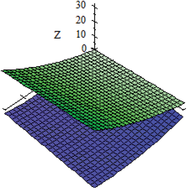
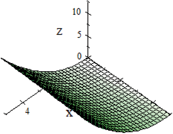
Then Φ(v,τ,γ)=[Φ∗(v,τ,γ),Φ∗(v,τ,γ)] for all 0≤γ≤1. For γ=0, we have the following:
Φ(v,τ,γ)=[v22−3v−τ,v22+3v+τ]
and its graph is given in Fig. 1.

Figure 1: Graph of Φ(v,τ,γ)=[Φ∗(v,τ,γ),Φ∗(v,τ,γ)] with γ=0
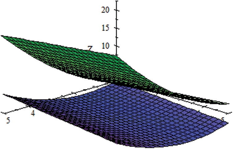
For γ=0.5, we have the following:
Φ(v,τ,γ)=[v22+3(−0.5)v+(−0.5)τ,v22+3(0.5)v+(0.5)τ]
and its graph is given in Fig. 2.

Figure 2: Graph of Φ(v,τ,γ)=[Φ∗(v,τ,γ),Φ∗(v,τ,γ)] with γ=0.5
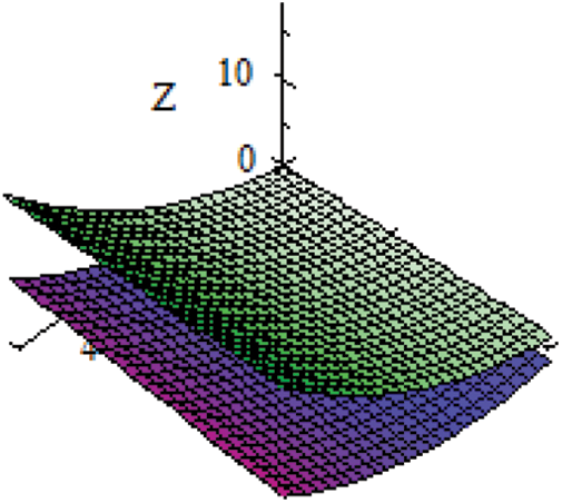
For γ=0.7, we have the following
Φ(v,τ,γ)=[v22+3(−0.3)v+(−0.3)τ,v22+3(0.3)v+(0.3)τ]
and its graph is given in Fig. 3.

Figure 3: Graph of Φ(v,τ,γ)=[Φ∗(v,τ,γ),Φ∗(v,τ,γ)] with γ=0.7
For γ=1, we have the following:
Φ(v,τ,γ)=[v22,v22]
and its graph is given in Fig. 4.

Figure 4: Graph of Φ(v,τ,γ)=[Φ∗(v,τ,γ),Φ∗(v,τ,γ)] with γ=1
4.2 Of Order 2Ψ
In this subsection, we solve fuzzy conformable heat equation and fuzzy conformable wave equation using fuzzy conformable double Laplace transform.
4.2.1 Heat Equation
Fuzzy conformable heat equation in one dimension has many forms such as
∂δ∂τδ(∂δΦ∂τδ)=α∂2Φ∂v2.
Also, this form has been used by some researchers
∂δΦ∂τδ=∂2Φ∂v2.
We use the fuzzy conformable heat equation in the form
∂δΦ∂τδ=α⊙∂2ΨΦ∂v2Ψ,Φ(v,0)=ϝ(v),Φ(0,τ)=h(τ),Φ(a,τ)=g(τ),
where Φ is a temperature of a rod of a constant-cross section and homogeneous material, lying along the axis, and α is a constant of diffusion. We have taken initial and boundary conditions as fuzzy numbers. For simplicity, we take α=1.
To solve fuzzy conformable heat equation with fuzzy conformable double Laplace transform, the procedure is as follows:
First, apply fuzzy conformable double Laplace transform on both sides of the fuzzy conformable heat equation.
ℓΨvℓδτ[∂2ΨΦ(v,τ)∂v2Ψ]=ℓΨvℓδτ[∂δΦ(v,τ)∂τδ].
The fuzzy conformable heat equation is changed into the conformable boundary value problem.
1. When Φ(v,τ) is differentiable of the type (δ−1), we have four cases associated with the four types of derivatives with respect to order 2Ψ.
Case 1: If Φ and ∂ΨΦ(v,τ)∂vΨ are the strongly generalized conformable partial differentiable of the type (Ψ−1), then we obtain the following system of equations
r12ϕ∗(r1,r2)−r1ϕ∗(0,r2)−∂Ψϕ∗(0,r2)∂vΨ=r2ϕ∗(r1,r2,γ)−ϕ∗(r1,0,γ),r12ϕ∗(r1,r2)−r1ϕ∗(0,r2)−∂Ψϕ∗(0,r2)∂vΨ=r2ϕ∗(r1,r2,γ)−ϕ∗(r1,0,γ).
Case 2: If Φ and ∂ΨΦ(v,τ)∂vΨ are the strongly generalized conformable partial differentiable of the type (Ψ−2), then we obtain the following system of equations
r12ϕ∗(r1,r2)−r1ϕ∗(0,r2)−∂Ψϕ∗(0,r2)∂vΨ=r2ϕ∗(r1,r2,γ)−ϕ∗(r1,0,γ),r12ϕ∗(r1,r2)−r1ϕ∗(0,r2)−∂Ψϕ∗(0,r2)∂vΨ=r2ϕ∗(r1,r2,γ)−ϕ∗(r1,0,γ).
Case 3: If Φ is the strongly generalized conformable partial differentiable of the type (Ψ−2) and ∂ΨΦ(v,τ)∂vΨ is differentiable of the type (Ψ -1), then by applying fuzzy conformable double Laplace transform on both sides, we obtain the following system of equations
r12ϕ∗(r1,r2)−r1ϕ∗(0,r2)−∂Ψϕ∗(0,r2)∂vΨ=r2ϕ∗(r1,r2,γ)−ϕ∗(r1,0,γ),r12ϕ∗(r1,r2)−r1ϕ∗(0,r2)−∂Ψϕ∗(0,r2)∂vΨ=r2ϕ∗(r1,r2,γ)−ϕ∗(r1,0,γ).
Case 4: If Φ is the strongly generalized conformable partial differentiable of the type (Ψ−1) and ∂ΨΦ(v,τ)∂vΨ is differentiable of the type (Ψ−2), then by applying fuzzy conformable double Laplace transform on both sides, we obtain the following system of equations
r12ϕ∗(r1,r2)−r1ϕ∗(0,r2)−∂Ψϕ∗(0,r2)∂vΨ=r2ϕ∗(r1,r2,γ)−ϕ∗(r1,0,γ),r12ϕ∗(r1,r2)−r1ϕ∗(0,r2)−∂Ψϕ∗(0,r2)∂vΨ=r2ϕ∗(r1,r2,γ)−ϕ∗(r1,0,γ).
2. When Φ(v,τ) is strongly generalized conformable partial differentiable of the type (δ−2), we again have four cases associated with the four types of derivatives with respect to order 2Ψ.
Case 1: If Φ and ∂ΨΦ(v,τ)∂vΨ are the strongly generalized conformable partial differentiable of the type (Ψ−1), then we obtain the following system of equations
r12ϕ∗(r1,r2)−r1ϕ∗(0,r2)−∂Ψϕ∗(0,r2)∂vΨ=r2ϕ∗(r1,r2,γ)−ϕ∗(r1,0,γ),r12ϕ∗(r1,r2)−r1ϕ∗(0,r2)−∂Ψϕ∗(0,r2)∂vΨ=r2ϕ∗(r1,r2,γ)−ϕ∗(r1,0,γ).
Case 2: If Φ and ∂ΨΦ(v,τ)∂vΨ are the strongly generalized conformable partial differentiable of the type (Ψ−2), then we obtain the following system of equations
r12ϕ∗(r1,r2)−r1ϕ∗(0,r2)−∂Ψϕ∗(0,r2)∂vΨ=r2ϕ∗(r1,r2,γ)−ϕ∗(r1,0,γ),r12ϕ∗(r1,r2)−r1ϕ∗(0,r2)−∂Ψϕ∗(0,r2)∂vΨ=r2ϕ∗(r1,r2,γ)−ϕ∗(r1,0,γ).
Case 3: If Φ is the strongly generalized conformable partial differentiable of the type (Ψ−2) and ∂ΨΦ(v,τ)∂vΨ is differentiable of the type (Ψ−1), then by applying fuzzy conformable double Laplace transform on both sides, we obtain the following system of equations
r12ϕ∗(r1,r2)−r1ϕ∗(0,r2)−∂Ψϕ∗(0,r2)∂vΨ=r2ϕ∗(r1,r2,γ)−ϕ∗(r1,0,γ),r12ϕ∗(r1,r2)−r1ϕ∗(0,r2)−∂Ψϕ∗(0,r2)∂vΨ=r2ϕ∗(r1,r2,γ)−ϕ∗(r1,0,γ).
Case 4: If Φ is the strongly generalized conformable partial differentiable of the type (Ψ−1) and ∂ΨΦ(v,τ)∂vΨ is differentiable of the type (Ψ−2), then by applying fuzzy conformable double Laplace transform on both sides, we obtain the following system of equations
r12ϕ∗(r1,r2)−r1ϕ∗(0,r2)−∂Ψϕ∗(0,r2)∂vΨ=r2ϕ∗(r1,r2,γ)−ϕ∗(r1,0,γ),r12ϕ∗(r1,r2)−r1ϕ∗(0,r2)−∂Ψϕ∗(0,r2)∂vΨ=r2ϕ∗(r1,r2,γ)−ϕ∗(r1,0,γ).
Now, solving the above systems of equations and applying boundary conditions, and then implementing fuzzy conformable double Laplace inverse transform, we get the solution in the form Φ(v,τ,γ)=[Φ∗(v,τ,γ),Φ∗(v,τ,γ)].
Now, we interpret the benefits of our method with an example.
Example 4.3. Consider fuzzy conformable heat equation
∂δΦ∂τδ=∂2ΨΦ∂v2Ψ,Φ(v,0)=0,Φ(0,τ)=(−1,0,1),∂ΨΦ(0,τ)∂vΨ=(1,2,3).
Fuzzy conformable double Laplace transform implies eight cases of the above system. Here, we consider four nontrivial cases for the solution.
Case 1: If Φ and ∂ΨΦ∂vΨ are differentiable of the type (Ψ−1) with respect to v, and Φ is differentiable of the type (δ−1) with respect to τ, then by applying fuzzy conformable double Laplace transform on both sides, we obtain
ϕ∗(r1,r2,γ)=−r1r2(r2−r12)(γ−1)−(1+γ)r2(r2−r12),ϕ∗(r1,r2,γ)=−r1r2(r2−r12)(1−γ)−(3−γ)r2(r2−r12).
Case 2: If Φ and ∂ΨΦ∂vΨ are differentiable of the type (Ψ−1) with respect to v, and Φ is differentiable of the type (δ−2) with respect to τ, then by applying fuzzy conformable double Laplace transform on both sides, we obtain
ϕ∗(r1,r2,γ)=−r13r2(r22−r14)(γ−1)−r12(1+γ)r2(r22−r14)−r1(1−γ)(r22−r14)−(3−γ)(r22−r14),ϕ∗(r1,r2,γ)=−r1r22−r14(γ−1)−r2(1+γ)r1(r22−r14)−r13(1−γ)r2(r22−r14)−r12(3−γ)r2(r22−r14).
Case 3: When Φ and ∂ΨΦ∂vΨ are differentiable of type (Ψ−2) with respect to v, and Φ is differentiable of the type (δ−1) with respect to τ, then by applying fuzzy conformable double Laplace transform on both sides, we obtain
ϕ∗(r1,r2,γ)=−r1(1−γ)r22−r14−1+γr22−r14−r13(γ−1)r2(r22−r14)−r12(3−γ)(r22−r14),ϕ∗(r1,r2,γ)=−r13(1−γ)r2(r22−r14)−r12(1+γ)r2(r22−r14)−r1(γ−1)r22−r14−(3−γ)r22−r14.
Case 4: When Φ is differentiable of type (Ψ−1) with respect to v and ∂ΨΦ∂vΨ is differentiable of type (Ψ−2) with respect to v and Φ is differentiable of the type (δ−1) with respect to τ, then by applying fuzzy conformable double Laplace transform on both sides, we obtain
ϕ∗(r1,r2,γ)=−r13(γ−1)r2(r22−r14)−r12(1+γ)r2(r22−r14)−r1(γ−1)r22−r14−3−γr22−r14,ϕ∗(r1,r2,γ)=−r1(1−γ)r22−r14−1+γr22−r14−r13(1−γ)r2(r22−r14)−r12(3−γ)r2(r22−r14).
Fuzzy conformable double Laplace inverse can yield the required solutions.
4.2.2 Wave Equation
Let us consider the following 1D fuzzy conformable wave equation
∂2δΦ∂τ2δ=α2⊙∂2ΨΦ∂v2Ψ,Φ(v,0)=ψ(v),∂δΦ(v,0)∂τδ=ϝ(v),Φ(0,τ)=g(τ),∂ΨΦ(0,τ)∂vΨ=h(τ).
To solve the fuzzy conformable wave equation with the fuzzy conformable double Laplace transform, the procedure is as follows:
First, apply fuzzy conformable double Laplace transform on both sides of the fuzzy conformable wave equation. As a result, we have possible sixteen cases.
1. First, we take Φ(v,τ) and ∂Ψ(v,τ)∂vΨ as differentiable of the type (Ψ−1) with respect to v. It implies four associated cases.
Case 1: When Φ and ∂δΦ∂τδ are strongly generalized conformable partial differentiable of the type (δ−1), then we obtain the form
r22ϕ∗(r1,r2)−r2ϕ∗(r1,0)−∂δϕ∗(r1,0)∂τδ=r12ϕ∗(r1,r2)−r1ϕ∗(0,r2)−∂Ψϕ∗(0,r2)∂vΨ,r22ϕ∗(r1,r2)−r2ϕ∗(r1,0)−∂δϕ∗(r1,0)∂τδ=r12ϕ∗(r1,r2)−r1ϕ∗(0,r2)−∂Ψϕ∗(0,r2)∂vΨ.
Case 2: When Φ and ∂δΦ∂τδ are strongly generalized conformable partial differentiable of the type (δ−2), then we obtain the form
r22ϕ∗(r1,r2)−r2ϕ∗(r1,0)−∂δϕ∗(r1,0)∂τδ=r12ϕ∗(r1,r2)−r1ϕ∗(0,r2)−∂Ψϕ∗(0,r2)∂vΨ,r22ϕ∗(r1,r2)−r2ϕ∗(r1,0)−∂δϕ∗(r1,0)∂τδ=r12ϕ∗(r1,r2)−r1ϕ∗(0,r2)−∂Ψϕ∗(0,r2)∂vΨ.
Case 3: When Φ is strongly generalized conformable partial differentiable of the type (δ−1) and ∂δΦ∂τδ is strongly generalized conformable partial differentiable of the type (δ−2), then we obtain the form
r22ϕ∗(r1,r2)−r2ϕ∗(r1,0)−∂δϕ∗(r1,0)∂τδ=r12ϕ∗(r1,r2)−r1ϕ∗(0,r2)−∂Ψϕ∗(0,r2)∂vΨ,r22ϕ∗(r1,r2)−r2ϕ∗(r1,0)−∂δϕ∗(r1,0)∂τδ=r12ϕ∗(r1,r2)−r1ϕ∗(0,r2)−∂Ψϕ∗(0,r2)∂vΨ.
Case 4: When Φ is strongly generalized conformable partial differentiable of the type (δ−2) and ∂δΦ∂τδ is strongly generalized conformable partial differentiable of the type (δ−1), then we obtain the form
r22ϕ∗(r1,r2)−r2ϕ∗(r1,0)−∂δϕ∗(r1,0)∂τδ=r12ϕ∗(r1,r2)−r1ϕ∗(0,r2)−∂Ψϕ∗(0,r2)∂vΨ,r22ϕ∗(r1,r2)−r2ϕ∗(r1,0)−∂δϕ∗(r1,0)∂τδ=r12ϕ∗(r1,r2)−r1ϕ∗(0,r2)−∂Ψϕ∗(0,r2)∂vΨ.
2. Now, we take Φ(v,τ) and ∂ΨΦ(v,τ)∂vΨ as differentiable of the type (Ψ−2), then we have four associated cases.
Case 1: When Φ and ∂δΦ∂τδ are strongly generalized conformable partial differentiable of the type (δ−1), then we obtain the form
r22ϕ∗(r1,r2)−r2ϕ∗(r1,0)−∂δϕ∗(r1,0)∂τδ=r12ϕ∗(r1,r2)−r1ϕ∗(0,r2)−∂Ψϕ∗(0,r2)∂vΨ,r22ϕ∗(r1,r2)−r2ϕ∗(r1,0)−∂δϕ∗(r1,0)∂τδ=r12ϕ∗(r1,r2)−r1ϕ∗(0,r2)−∂Ψϕ∗(0,r2)∂vΨ.
Case 2: When Φ and ∂δΦ∂τδ are strongly generalized conformable partial differentiable of the type (δ−2), then we obtain the form
r22ϕ∗(r1,r2)−r2ϕ∗(r1,0)−∂δϕ∗(r1,0)∂τδ=r12ϕ∗(r1,r2)−r1ϕ∗(0,r2)−∂Ψϕ∗(0,r2)∂vΨ,r22ϕ∗(r1,r2)−r2ϕ∗(r1,0)−∂δϕ∗(r1,0)∂τδ=r12ϕ∗(r1,r2)−r1ϕ∗(0,r2)−∂Ψϕ∗(0,r2)∂vΨ.
Case 3: When Φ is strongly generalized conformable partial differentiable of the type (δ−1) and ∂δΦ∂τδ is strongly generalized conformable partial differentiable of the type (δ−2), then we obtain the form
r22ϕ∗(r1,r2)−r2ϕ∗(r1,0)−∂δϕ∗(r1,0)∂τδ=r12ϕ∗(r1,r2)−r1ϕ∗(0,r2)−∂Ψϕ∗(0,r2)∂vΨ,r22ϕ∗(r1,r2)−r2ϕ∗(r1,0)−∂δϕ∗(r1,0)∂τδ=r12ϕ∗(r1,r2)−r1ϕ∗(0,r2)−∂Ψϕ∗(0,r2)∂vΨ.
Case 4: When Φ is strongly generalized conformable partial differentiable of the type (δ−2) and ∂δΦ∂τδ is strongly generalized conformable partial differentiable of the type (δ−1), then we obtain the form
r22ϕ∗(r1,r2)−r2ϕ∗(r1,0)−∂δϕ∗(r1,0)∂τδ=r12ϕ∗(r1,r2)−r1ϕ∗(0,r2)−∂Ψϕ∗(0,r2)∂vΨ,r22ϕ∗(r1,r2)−r2ϕ∗(r1,0)−∂δϕ∗(r1,0)∂τδ=r12ϕ∗(r1,r2)−r1ϕ∗(0,r2)−∂Ψϕ∗(0,r2)∂vΨ.
3. As a third option, we take Φ as strongly generalized conformable partial differentiable of the type (Ψ−2) and ∂ΨΦ∂vΨ as strongly generalized conformable partial differentiable of the type (Ψ−1), which enables us to have four cases associated with the four types of derivative for τ, which are given by
Case 1: When Φ and ∂δΦ∂τδ are strongly generalized conformable partial differentiable of the type (δ−1), then we obtain the form
r22ϕ∗(r1,r2)−r2ϕ∗(r1,0)−∂δϕ∗(r1,0)∂τδ=r12ϕ∗(r1,r2)−r1ϕ∗(0,r2)−∂Ψϕ∗(0,r2)∂vΨ,r22ϕ∗(r1,r2)−r2ϕ∗(r1,0)−∂δϕ∗(r1,0)∂τδ=r12ϕ∗(r1,r2)−r1ϕ∗(0,r2)−∂Ψϕ∗(0,r2)∂vΨ.
Case 2: When Φ and ∂δΦ∂τδ are strongly generalized conformable partial differentiable of the type (δ−2), then we obtain the form
r22ϕ∗(r1,r2)−r2ϕ∗(r1,0)−∂δϕ∗(r1,0)∂τδ=r12ϕ∗(r1,r2)−r1ϕ∗(0,r2)−∂Ψϕ∗(0,r2)∂vΨ,r22ϕ∗(r1,r2)−r2ϕ∗(r1,0)−∂δϕ∗(r1,0)∂τδ=r12ϕ∗(r1,r2)−r1ϕ∗(0,r2)−∂Ψϕ∗(0,r2)∂vΨ.
Case 3: When Φ is strongly generalized conformable partial differentiable of the type (δ−1) and ∂δΦ∂τδ is strongly generalized conformable partial differentiable of the type (δ−2), then we obtain the form
r22ϕ∗(r1,r2)−r2ϕ∗(r1,0)−∂δϕ∗(r1,0)∂τδ=r12ϕ∗(r1,r2)−r1ϕ∗(0,r2)−∂Ψϕ∗(0,r2)∂vΨ,r22ϕ∗(r1,r2)−r2ϕ∗(r1,0)−∂δϕ∗(r1,0)∂τδ=r12ϕ∗(r1,r2)−r1ϕ∗(0,r2)−∂Ψϕ∗(0,r2)∂vΨ.
Case 4: When Φ is strongly generalized conformable partial differentiable of the type (δ−2) and ∂δΦ∂τδ is strongly generalized conformable partial differentiable of the type (δ−1), then we obtain the form
r22ϕ∗(r1,r2)−r2ϕ∗(r1,0)−∂δϕ∗(r1,0)∂τδ=r12ϕ∗(r1,r2)−r1ϕ∗(0,r2)−∂Ψϕ∗(0,r2)∂vΨ,r22ϕ∗(r1,r2)−r2ϕ∗(r1,0)−∂δϕ∗(r1,0)∂τδ=r12ϕ∗(r1,r2)−r1ϕ∗(0,r2)−∂Ψϕ∗(0,r2)∂vΨ.
4. In the fourth case, we take Φ as strongly generalized conformable partial differentiable of the type (Ψ−1) and ∂ΨΦ∂vΨ as strongly generalized conformable partial differentiable of the type (Ψ−2), which enables us to have four cases associated with the four types of derivative for τ, which are given by
Case 1: When Φ and ∂δΦ∂τδ are strongly generalized conformable partial differentiable of the type (δ−1), then we obtain the form
r22ϕ∗(r1,r2)−r2ϕ∗(r1,0)−∂δϕ∗(r1,0)∂τδ=r12ϕ∗(r1,r2)−r1ϕ∗(0,r2)−∂Ψϕ∗(0,r2)∂vΨ,r22ϕ∗(r1,r2)−r2ϕ∗(r1,0)−∂δϕ∗(r1,0)∂τδ=r12ϕ∗(r1,r2)−r1ϕ∗(0,r2)−∂Ψϕ∗(0,r2)∂vΨ.
Case 2: When Φ and ∂δΦ∂τδ are strongly generalized conformable partial differentiable of the type (δ−2), then we obtain the form
r22ϕ∗(r1,r2)−r2ϕ∗(r1,0)−∂δϕ∗(r1,0)∂τδ=r12ϕ∗(r1,r2)−r1ϕ∗(0,r2)−∂Ψϕ∗(0,r2)∂vΨ,r22ϕ∗(r1,r2)−r2ϕ∗(r1,0)−∂δϕ∗(r1,0)∂τδ=r12ϕ∗(r1,r2)−r1ϕ∗(0,r2)−∂Ψϕ∗(0,r2)∂vΨ.
Case 3: When Φ is strongly generalized conformable partial differentiable of the type (δ−2) and ∂δΦ∂τδ is strongly generalized conformable partial differentiable of the type (δ−1), then we obtain the form
r22ϕ∗(r1,r2)−r2ϕ∗(r1,0)−∂δϕ∗(r1,0)∂τδ=r12ϕ∗(r1,r2)−r1ϕ∗(0,r2)−∂Ψϕ∗(0,r2)∂vΨ,r22ϕ∗(r1,r2)−r2ϕ∗(r1,0)−∂δϕ∗(r1,0)∂τδ=r12ϕ∗(r1,r2)−r1ϕ∗(0,r2)−∂Ψϕ∗(0,r2)∂vΨ.
Case 4: When Φ is strongly generalized conformable partial differentiable of the type (δ−1) and ∂δΦ∂τδ is strongly generalized conformable partial differentiable of the type (δ−2), then we obtain the form
r22ϕ∗(r1,r2)−r2ϕ∗(r1,0)−∂δϕ∗(r1,0)∂τδ=r12ϕ∗(r1,r2)−r1ϕ∗(0,r2)−∂Ψϕ∗(0,r2)∂vΨ,r22ϕ∗(r1,r2)−r2ϕ∗(r1,0)−∂δϕ∗(r1,0)∂τδ=r12ϕ∗(r1,r2)−r1ϕ∗(0,r2)−∂Ψϕ∗(0,r2)∂vΨ.
Solving the above systems of equations, and apply the fuzzy conformable double Laplace inverse, we can get the solution in the form Φ(v,τ,γ)=[Φ∗(v,τ,γ),Φ∗(v,τ,γ)].
Now, we present an example of the fuzzy conformable wave equation to demonstrate the validity of our results.
Example 4.4. Consider fuzzy conformable wave equation in one dimension is
∂2δΦ∂τ2δ=∂2ΨΦ∂v2Ψ,Φ(0,τ)=(0,1,2),∂ΨΦ(0,τ)∂vΨ=(1,2,3),∂δΦ∂τδ(v,0)=0,Φ(v,0)=0.
Fuzzy conformable double Laplace transform implies sixteen possibilities. We consider here only nontrivial four cases for the solution.
Case 1: When both Φ and ∂δΦ∂τδ are strongly generalized conformable partial differentiable of the type (δ−1) and Φ(v,τ),∂ΨΦ∂vΨ are differentiable of the type (Ψ−1), then we obtain
ϕ∗(r1,r2,γ)=−r2r1(r12−r22)(γ)−(1+γ)r1(r12−r22),ϕ∗(r1,r2,γ)=−r2r1(r12−r22)(2−γ)−(3−γ)r1(r12−r22).
Case 2: When Φ and ∂δΦ∂τδ is differentiable of type (δ−1) with respect to τ and Φ(v,τ),∂ΨΦ∂vΨ are differentiable of the type (Ψ−2), then we obtain
ϕ∗(r1,r2,γ)=−(γ)r22r1(r14−r24)−(1+γ)r22r1(r14−r24)−r1r2r14−r24(2−γ)+r1r14−r24(3−γ),ϕ∗(r1,r2,γ)=γr1r14−r24−(1+γ)r1r14−r24+r23r1(r14−r24)(2−γ)−r22r1(r14−r24)(3−γ).
Case 3: When Φ and ∂δΦ∂τδ are differentiable of type (δ−2) and Φ(v,τ),∂ΨΦ∂vΨ are differentiable of the type (Ψ−1), then we obtain
ϕ∗(r1,r2,γ)=−(2−γ)r1r2r14−r24−(3−γ)r1r14−r24−r23r1(r14−r24)(γ)−r22r1(r14−r24)(1+γ),ϕ∗(r1,r2,γ)=−(2−γ)r23r1(r14−r24)−(3−γ)r22r1(r14−r24)−r1r2r14−r24(1+γ)−r1r14−r24(1+γ).
Case 4: When Φ is differentiable of type (δ−1) and ∂δΦ∂τδ is differentiable of type (δ−2) and Φ(v,τ),∂ΨΦ∂vΨ are differentiable of the type (Ψ−1), then we obtain
ϕ∗(r1,r2,γ)=−(2−γ)r22r1(r14−r24)−(3−γ)r22r1(r14−r24)−r1r2r14−r24(γ)+r1r14−r24(1+γ),ϕ∗(r1,r2,γ)=(2−γ)r1r14−r24−(3−γ)r1r14−r24+r23r1(r14−r24)(γ)−r22r1(r14−r24)(1+γ).
After solving the above system, and applying the fuzzy conformable double Laplace inverse, we can get the required solution.
5 Conclusion
We have introduced the fuzzy double Laplace transform and fuzzy conformable double Laplace transform. Also, related properties and theorems for derivatives and integrals of the transform are presented. We apply the fuzzy conformable double Laplace transform in this manuscript to obtain the solutions of fuzzy conformable PDEs (both in 1D and 2D). The fuzzy conformable PDEs are solved using this approach without transforming into conformable partial differential equations, so it is not important to find a solution to the partial differential equation. This is the greatest benefit of this system. The double Laplace transformation technique, therefore, is very convenient and effective. However, explicit solutions for each system require inverse double Laplace transform, which is complicated to solve. In future work, we will obtain numerical solution methods to overcome these complications.
Acknowledgement: The authors wish to express their appreciation to the reviewers for their helpful suggestions which greatly improved the presentation of this paper.
Funding Statement: The author Manar A. Alqudah would like to thank Princess Nourah bint Abdulrahman University Researchers Supporting Project No. (PNURSP2023R14), Princess Nourah bint Abdulrahman University, Riyadh, Saudi Arabia.
Conflicts of Interest: The authors declare that they have no conflicts of interest to report regarding the present study.
References
1. Alderremy, A., Abdel-Gawad, H., Saad, K. M., Aly, S. (2021). New exact solutions of time conformable fractional Klein Kramer equation. Optical and Quantum Electronics, 53(12), 1–14. DOI 10.1007/s11082-021-03343-7. [Google Scholar] [CrossRef]
2. Alderremy, A., Gómez-Aguilar, J., Aly, S., Saad, K. M. (2021). A fuzzy fractional model of coronavirus (COVID-19) and its study with legendre spectral method. Results in Physics, 21, 103773. DOI 10.1016/j.rinp.2020.103773. [Google Scholar] [CrossRef]
3. Younus, A., Asif, M., Atta, U., Bashir, T., Abdeljawad, T. (2021). Some fundamental results on fuzzy conformable differential calculus. Journal of Fractional Calculus and Nonlinear Systems, 2(2), 31–61. DOI 10.48185/jfcns.v2i2.341. [Google Scholar] [CrossRef]
4. Afariogun, D., Mogbademu, A., Olaoluwa, H. (2021). On fuzzy henstock-kurzweil-stieltjes diamond double integral on time scales. Journal of Mathematical Analysis and Modeling, 2(2), 38–49. DOI 10.48185/jmam.v2i2.295. [Google Scholar] [CrossRef]
5. Hashim, D. J., Jameel, A. F., Ying, T. Y., Alomari, A., Anakira, N. (2022). Optimal homotopy asymptotic method for solving several models of first order fuzzy fractional ivps. Alexandria Engineering Journal, 61(6), 4931–4943. DOI 10.1016/j.aej.2021.09.060. [Google Scholar] [CrossRef]
6. Jameel, A., Anakira, N., Shather, A., Saaban, A., Alomari, A. (2020). Numerical algorithm for solving second order nonlinear fuzzy initial value problems. International Journal of Electrical and Computer Engineering, 10(6), 6497–6506. DOI 10.11591/ijece.v10i6.pp6497-6506. [Google Scholar] [CrossRef]
7. Kilicman, A., Gadain, H. (2009). An application of double laplace transform and double sumudu transform. Lobachevskii Journal of Mathematics, 30(3), 214–223. DOI 10.1134/S1995080209030044. [Google Scholar] [CrossRef]
8. Ali, A., Suwan, I., Abdeljawad, T., Abdullah (2022). Numerical simulation of time partial fractional diffusion model by laplace transform. AIMS Mathematics, 7(2), 2878–2890. DOI 10.3934/math.2022159. [Google Scholar] [CrossRef]
9. Arqub, O. A., Al-Smadi, M. (2020). Fuzzy conformable fractional differential equations: Novel extended approach and new numerical solutions. Soft Computing, 24(16), 12501–12522. DOI 10.1007/s00500-020-04687-0. [Google Scholar] [CrossRef]
10. Allahviranloo, T., Gouyandeh, Z., Armand, A., Hasanoglu, A. (2015). On fuzzy solutions for heat equation based on generalized hukuhara differentiability. Fuzzy Sets and Systems, 265, 1–23. DOI 10.1016/j.fss.2014.11.009. [Google Scholar] [CrossRef]
11. Rahimi Chermahini, S., Asgari, M. S. (2021). Analytical fuzzy triangular solutions of the wave equation. Soft Computing, 25(1), 363–378. DOI 10.1007/s00500-020-05146-6. [Google Scholar] [CrossRef]
12. Gouyandeh, Z., Allahviranloo, T., Abbasbandy, S., Armand, A. (2017). A fuzzy solution of heat equation under generalized hukuhara differentiability by fuzzy Fourier transform. Fuzzy Sets and Systems, 309, 81–97. DOI 10.1016/j.fss.2016.04.010. [Google Scholar] [CrossRef]
13. Dhunde, R. R., Waghmare, G. (2016). Double laplace transform method for solving space and time fractional telegraph equations. International Journal of Mathematics and Mathematical Sciences, 2016, 1–7. DOI 10.1155/2016/1414595. [Google Scholar] [CrossRef]
14. Allahviranloo, T., Ahmadi, M. B. (2010). Fuzzy laplace transforms. Soft Computing, 14(3), 235–243. DOI 10.1007/s00500-008-0397-6. [Google Scholar] [CrossRef]
15. Ahmad, L., Farooq, M., Abdullah, S. (2014). Solving nth order fuzzy differential equation by fuzzy laplace transform. arXiv preprint arXiv:1403.0242. [Google Scholar]
16. Ahmad, L., Farooq, M., Abdullah, S. (2016). Solving forth order fuzzy differential equation by fuzzy laplace transform. Annals of Fuzzy Mathematics and Informatics, 12, 449–468. [Google Scholar]
17. Salahshour, S., Allahviranloo, T. (2013). Applications of fuzzy laplace transforms. Soft Computing, 17(1), 145–158. DOI 10.1007/s00500-012-0907-4. [Google Scholar] [CrossRef]
18. Salahshour, S., Haghi, E. (2010). Solving fuzzy heat equation by fuzzy laplace transforms. International Conference on Information Processing and Management of Uncertainty in Knowledge-Based Systems, Dortmund, Germany, Springer. [Google Scholar]
19. Abdeljawad, T. (2015). On conformable fractional calculus. Journal of Computational and Applied Mathematics, 279, 57–66. DOI 10.1016/j.cam.2014.10.016. [Google Scholar] [CrossRef]
20. Eltayeb, H., Mesloub, S., Abdalla, Y. T., Kılıçman, A. (2019). A note on double conformable laplace transform method and singular one dimensional conformable pseudohyperbolic equations. Mathematics, 7(10), 949. DOI 10.3390/math7100949. [Google Scholar] [CrossRef]
21. Silva, F. S., Moreira, D. M., Moret, M. A. (2018). Conformable Laplace transform of fractional differential equations. Axioms, 7(3), 55. [Google Scholar]
22. Younus, A., Asif, M., Atta, U., Bashir, T., Abdeljawad, T. (2021). Analytical solutions of fuzzy linear differential equations in the conformable setting. Journal of Fractional Calculus and Nonlinear Systems, 2(2), 13–30. DOI 10.48185/jfcns.v2i2.342. [Google Scholar] [CrossRef]
23. Debnath, L. (2016). The double laplace transforms and their properties with applications to functional, integral and partial differential equations. International Journal of Applied and Computational Mathematics, 2(2), 223–241. DOI 10.1007/s40819-015-0057-3. [Google Scholar] [CrossRef]
24. Özkan, O., Kurt, A. (2018). On conformable double laplace transform. Optical and Quantum Electronics, 50(2), 1–9. [Google Scholar]
25. Armand, A., Allahviranloo, T., Gouyandeh, Z. (2018). Some fundamental results on fuzzy calculus. Iranian Journal of Fuzzy Systems, 15(3), 27–46. [Google Scholar]

 Submit a Paper
 Propose a Special lssue
 Open Access
 View Full Text
 Download PDF
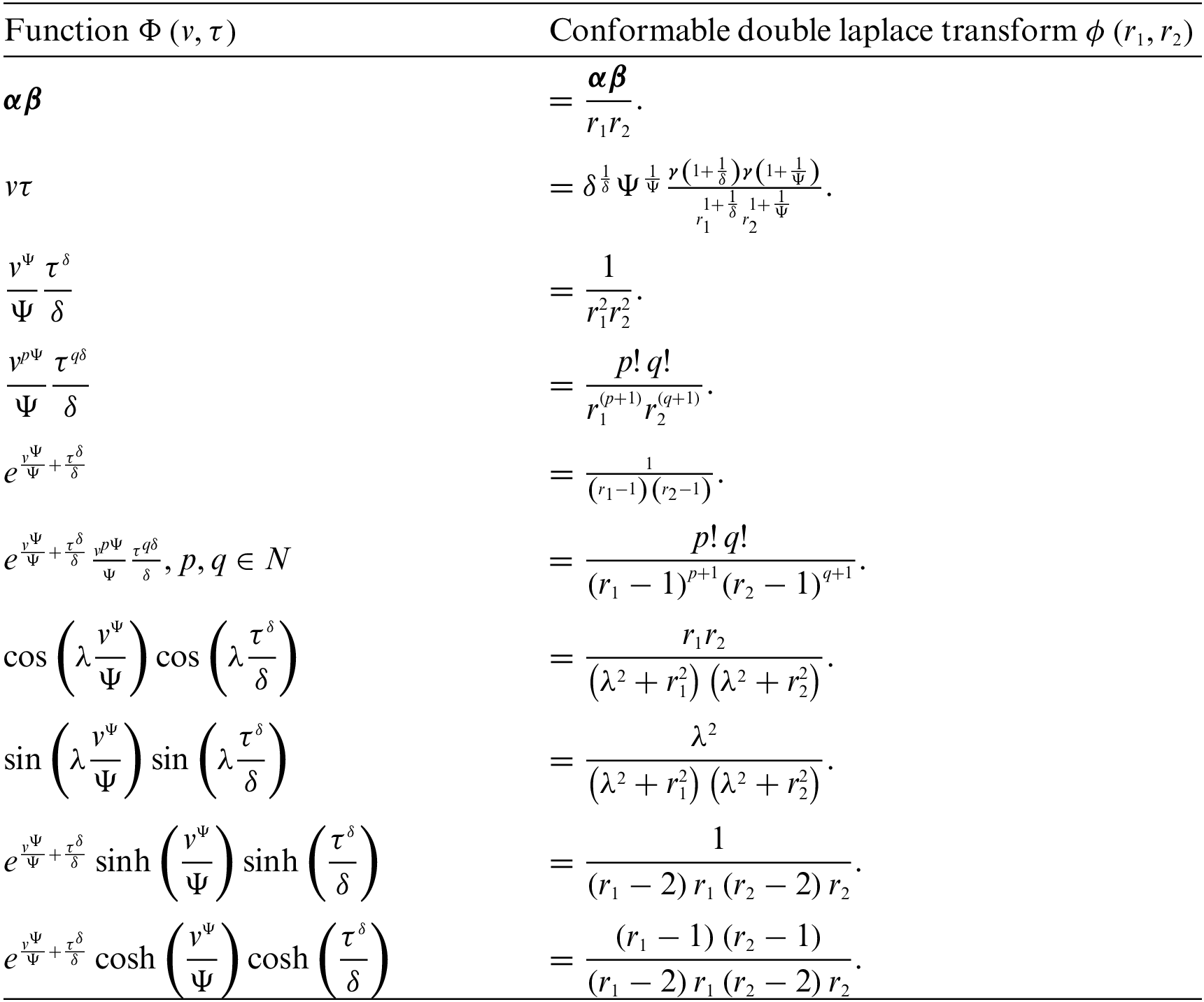
 Copyright © 2023 The Author(s). Published by Tech Science Press.
 Downloads
 Citation Tools