Change Point Detection for Process Data Analytics Applied to a Multiphase Flow Facility

1  Introduction

In process industries, the operating conditions of a process can change from time to time due to various reasons, such as the change of the scheduled production or the demand of the market. Nevertheless, many of the changes in the operating conditions are not explicitly recorded by the process historian; sometimes such information about the changes is indirectly stored by a combination of the alarm and event and the time trends of process variables. It may be possible for process experts to label the multiple modes or phases in the process manually; however the effort required will be enormous especially when the dataset is large. Therefore, an automated, unsupervised solution that can divide a large dataset into segments that correspond to different operating conditions is of interest and value to the industrial application.

The topic of Change point detection (CPD) has become more and more relevant as time series datasets increase in size and often contain repeated patterns. In the context of process data analytics, change points in the time series of process variables may have important indications about the process operation. For example, in a batch process, the change points can correspond to the operations and phases defined by the batch recipe. Identifying change points can assist labelling of the time series data. To detect the change points, a number of algorithms have been developed based on various principles, with application areas such as sensor signals, financial data or traffic modelling. Reference [1–7] The principles differ in solution exactness due to computational complexity and in formulating a cost function which determines how the change points are defined.

The first work on change point detection was done by Page [5,6] where piecewise identically distributed datasets were studied. The objective was to identify various features in the independent and non-overlapping segments. The mathematical background of change point detection can be found in work by Basseville et al. [8]. Examples of the features can be each data segment’s mean, variance, and distribution function. Detection of change points can either be done in real-time or in retrospect, and for a single signal or in multiple dimensions. The real time approach is generally known as online detection, while the retrospective approach is known as offline detection. This paper is based on offline detection, meaning all data is available for the entire time interval under investigation. Many CPD algorithms are generalised for usage on multi-dimensional data [7] whereas one-dimensional data can be seen as a special case. This paper focuses on one-dimensional time dependent data, where results are more intuitive and common in real world settings. Another important assumption in CPD algorithms is whether the total number of change points in a dataset is known beforehand. This work assumes that the number of change points is not known.

Recent research on change point detection is presented in [9,10]. Various CPD methods have been applied to a vast spread of areas, stretching from sensor signals [2] to natural language processing [11]. Some CPD methods have also been implemented for financial analysis [3] and network systems [4], where the algorithms are able to detect changes in the underlying setting. Change point detection has also been applied to chemical processes [1], where the change points in the mean of the data from chemical processes are considered to represent the changed quality of production. This illustrates the usability of change point detection and shows the need for domain expert knowledge to confirm that the algorithms make correct predictions.

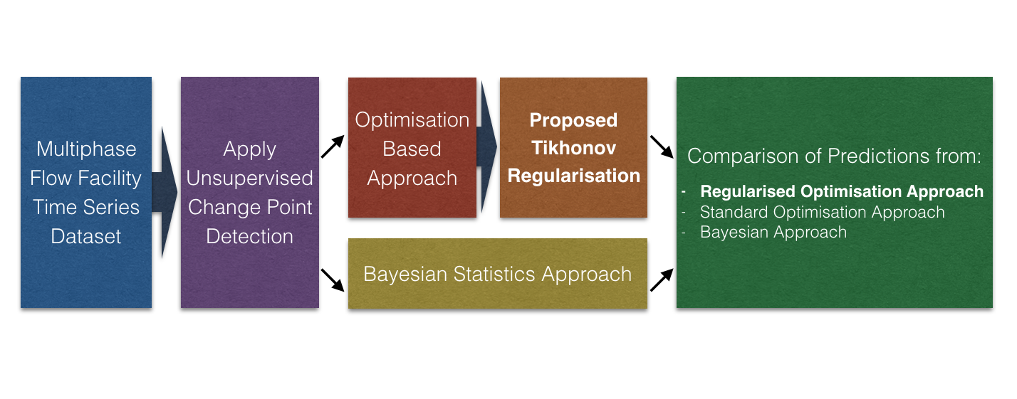
The current work is based on numerical testing of two approaches for CPD: the optimisation approach, with and without regularisation, and the Bayesian approach. Both approaches are tested on real world data from a multi-phase flow facility. These approaches are developed and studied separately in previous studies [7,12]. Performance comparison and the evaluation of both approaches’ computational efficiency form this work’s foundation. In extension to the existing work, presented in [7], new cost functions based on regularisation can be implemented. Some examples where regularisation techniques are used in machine learning algorithms are presented in [13–15]. For the Bayesian approach, the work by Fearnhead [12] describes the mathematics behind the algorithm. These two approaches have been studied separately and this work aims to compare the predictions made by the two approaches in a specific setting of a real world example. The methods presented by van Den Burg et al. [16] are used for numerical comparison, along with metrics specified by Truong et al. [7].

Using the same real world example, the paper also focuses on how regularised cost functions can improve change point detection compared to the performance of common change point detection algorithms. The contributions of the paper include the following:

1.    Study of regularised cost functions for CPD that can handle the ill-posed problem in noisy datasets.

2.    Application of various CPD algorithms to a dataset from a multi-phase process to demonstrate that CPD algorithms can identify the changes in the operating mode and label the data.

3.    Numerical verification of improvement in the performance of CPD using regularised cost functions when applied to real-life, noisy data.

This work is structured as follows: first the appropriate notation and definitions are introduced. Then, the two approaches for unsupervised CPD are derived separately in Section 2 along with the metrics used for comparison. In this section, the background theory of the completeness for ill-posed problems along with the proposed regularised cost functions are also introduced. The real life dataset, the testing procedure and the results of the experiment are presented in Section 3. A discussion is held in Section 4 and a summary of findings and conclusions are given in Section 5.

2  Background

In this section we provide the background knowledge for the two unsupervised CPD approaches. The section first presents the notations and definitions used in the paper, followed by the introduction to the optimisation-based CPD approach. Several elements of the optimisation approach, such as the problem formulation, the cost function and the search method, are also presented and the common cost functions are defined. The need of regularisation for CPD is discussed along with the proposed regularised cost functions. Then the Bayesian CPD approach is derived from Bayes’ formula using the same notations. It is demonstrated that, although the formulations of the two CPD approaches are different, the results obtained by both methods are similar, enabling the performance evaluation and comparison. Finally, the metrics used for evaluating the performance of change point detection are introduced.

2.1 Notation and Definition

Let us now introduce the notations used in the work. Fig. 1 shows multiple change points (τ0,τ1,…,τK+1) and the segments (S1,S2,…,SK+1), defined by the change points, and is an example of a univariate time-series dataset. Since the CPD approaches are unsupervised and do not require prior knowledge about the true change points, the target is to identify the time stamps τ0 to τK+1 given the time series.

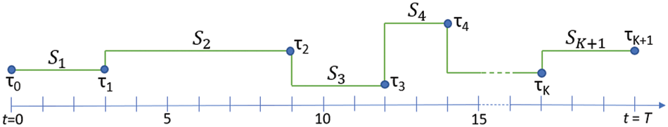
Figure 1: Illustration of used notation. In the figure, we see how K intermediate change points are present on a time interval t∈[0,T], where we note that τ0 and τK+1 are synthetic change points

Throughout the work we are working in the time domain [0,T]⊂N which is discretised with ti∈[0,T],i=0,1,…,n. The signal value at time ti is given by yti:=y(ti). The time points are equidistant, meaning ti+1=ti+dt, with dt=Tn−1,∀i. A set of K change points is denoted by T and is a subset of time indices {1,2,…,n}. The individual change points are indicated as τj, with j∈{0,1,…,K,K+1}, where τ0=0 and τK+1=T. With this definition the first and the final time point being implicit change points, we have K intermediate change points (|T|=|{τ1,…,τK}|=K). A segment of the signal from a to b is denoted as ya:b, where y0:T means the entire signal. With the introduced notation for change points, the segment Sj between change points τj−1 and τj is defined as Sj:=[τj−1,τj],|Sj|=τj−τj−1. Sj is the j-th non-overlapping segment in the signal, j∈{1,…,K+1}, see Fig. 1. Note that the definition for Sj does not hold for j=0, since this is the first change point.

As the goal is to identify whether a change has occurred in the signal, a proper definition of the term change point is needed along with clarification of change point detection. Change point detection is closely related to change point estimation (also known as change point mining, see [17,18]). According to Aminikhanghahi and Cook [19], change point estimation tries to model and interpret known changes in time series, while change point detection tries to identify whether a change has occurred [19]. This illustrates that we will not focus on the change points’ characteristics, but rather if a change point exists or not.

One challenge is identifying the number of change points in a given time series. A CPD algorithm is expected to detect enough change points whilst not over-fitting the data. If the number of change points is known beforehand the problem is merely the best fit problem. On the other hand, if the number of change points is not known, the problem can be seen as an optimisation problem with a penalty term for every added change point, or as enforcing a threshold when we are certain enough that a change point exists. It is evident that we need clear definitions of change points in order to detect them. The definitions for change point and change point detection are defined below and will be used throughout this work.

Definition 2.1 (Change point). A change point represents a transition between different states in a signal or dataset. If two consecutive segments ytl:ti and yti,tm, tl<ti<tm,l,i,m=0,…,n have a distinct change in features or if yti is a local extreme point (i.e., minimum or maximum1), then, τj=ti,j=0,1,…,K,K+1 is a change point between the two segments.

We note that the meaning of a distinct change in this definition is different for different CPD methods, and it is discussed in detail in Section 3. In the context of process data analytics, some change points are of interest for domain experts but may not follow Definition 1, hence difficult to identify. These change points are referred to as domain specific change points and are defined below.

Definition 2.2 (Change point, domain specific). For some process data, a change point is where a phase in the process starts or ends. These points can be indicated in the data, or be the points in the process of specific interest without a general change in data features.

Finally, we give one more definition of CPD for the case of available information about the probability distribution of a stochastic process.

Definition 2.3 (Change point detection). Identification of timestamps when the probability distribution of a stochastic process or time series segment changes. This concerns detecting whether or not a change has occurred, or whether several changes might have occurred, and identifying the timestamps of any such changes.

2.2 Optimisation Approach

Solving the task of identifying change points in a time series can be done by formulating as an optimisation problem. A detailed presentation of the framework is given in the work by Truonga et al. [7], while only a brief description is presented here. The purpose is to identify all the change points, without detecting fallacious ones. Therefore, the problem is formulated as an optimisation problem, where we strive to minimise the cost of segments and penalty per added change point. We need this penalty since we do not know how many change points will be presented. Mathematically, the non-regularised optimisation problem is formulated as

minTV(T)+pen(T)=minT∑j=1Kc(yτj:τj+1)+β|T|,(1)

while the regularised analogy is

minTV(T)+pen(T)+reg(T)=minT∑j=1Kc(yτj:τj+1)+β|T|+γ[T].(2)

Here, V(T) represents a cost function, pen(T) is a linear penalty function with constant β and reg(T) is a regularisation term in the appropriate norm in the time space [0,T] with the regularisation parameter γ.

To solve the optimisation problem (1), we need to combine three components: the search method, the cost function and the penalty term. Fig. 2 shows a schematic view of how the search method, cost function and penalty term create components of a CPD algorithm. Numerous combinations of components can be chosen for the problem (1). Fig. 2 also illustrates which methods will be studied in this work. The two methods for search directions and cost functions are presented in separate sections, while the choice of penalty function is kept brief. A common choice of penalty function is a linear penalty, which means each added change point τj corresponds to a penalty of β. A summary of other combinations are presented in Table 2 in the work by Truonga et al. [7].

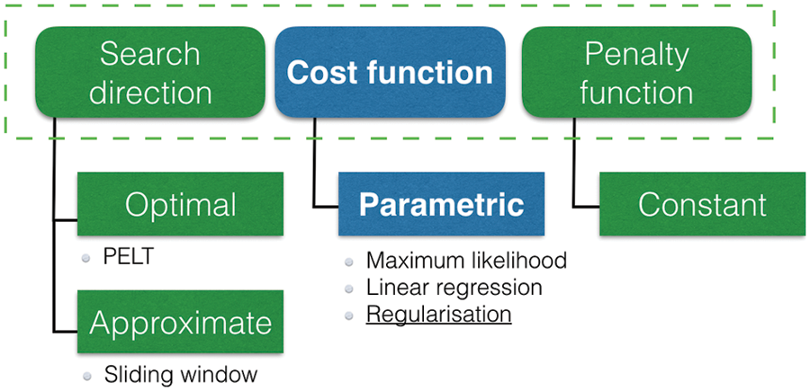
Figure 2: Illustration of the components used in the optimisation approach for change point detection. The focus of the paper is the cost function with regularisation

2.2.1 Search Direction

The search method poses a trade-off between accuracy and computational complexity. In CPD there are two main approaches used for this, optimal and approximate, see Fig. 2. The problem formulated in Eq. (1) should be solved for an unknown K, where the penalty function can be chosen as a constant function, pen(⋅)=β. The search method used for this special case is known as Pruned Exact Linear Time (abbreviated PELT) and implements a pruning rule. The pruning rule states that for two indices s and t, s<t<T, if the following condition holds

[minTV(T,y0:s)+β|T|]+c(ys:t)≥[minTV(T,y0:t)+β|T|],(3)

then s cannot be the last change point. Intuitively, the algorithm compares if it is beneficial to add another change point between s and t. If the cost of a segment ys:t is greater than the cost of two separated segments ys:τ, yτ+1:t and the additional penalty β, then there is a change point τ present between indices s and t. The PELT-algorithm is presented in Algorithm 1 in [20], and has a time complexity O(T) [7]. A drawback of this algorithm is that it can become computationally expensive for large datasets with many time stamps t.

An alternative approach is to use an approximate search direction algorithm to reduce complexity. To reduce the number of performed calculations, an approximate search direction can be used, where partial detection is common. There are multiple options available to approximate the search direction; some are studied by Troung et al. [7]. This paper focuses on one approach, the window based approximation. A frequently used technique is the Window-sliding algorithm (denoted as WIN-algorithm), when the algorithm returns an estimated change point in each iteration. Similar to the concept used in the PELT-algorithm, the value of the cost function between segments is compared. This is known as the discrepancy between segments and is defined as

Disc(yt−w:t,yt:t+w)=c(yt−w:t+w)−(c(yt−w:t)+c(yt:t+w)),(4)

where w is defined as half of the window width. Intuitively, this is merely the reduced cost of adding a change point at t in the middle of the window. The discrepancy is calculated for all w≤t≤T−w. When all calculations are done, the peaks of the discrepancy values are selected as the most profitable change points. The algorithm is provided in Algorithm 2 in [20]. There are other approximate search directions, which are not covered in this work, presented by Trounga et al. [7]. For this work, the PELT-algorithm is used for the optimal approach and the WIN-algorithm is used for the approximate approach.

2.2.2 Common Cost Functions

The cost function can decide which feature changes are detected in the data. In other words, the cost function measures the homogeneity. There are two approaches for defining a cost function: parametric and non-parametric. The respective approaches assume either that there is an underlying distribution in the data, or that there is no distribution in the data. This work focuses on the parametric cost functions, for three sub-techniques illustrated in Fig. 2. The three techniques, maximum likelihood estimation, linear regression and regularisation, are introduced in later sections with corresponding cost function definitions.

Maximum Likelihood Estimation (MLE) is a powerful tool with a wide application area in statistics. MLE finds the values of the model parameters that maximise the likelihood function f(y|θ) over the parameter space Θ such that MLE(y)=maxθ∈Θf(y|θ), where y is observed data and θ∈Θ is a vector of parameters. In the setting of change point detection, we assume the samples are independent random variables, linked to the distribution of a segment. This means that for all t∈[0,T], the sample

yt∼∑j=0Kf(⋅|θj)1(τj<t<τj+1),(5)

where θj is a segment specific parameter for the distribution. The function 1(⋅) is the delta function δ([τj,τj+1]), and is equal to one if sample yt belongs to segment j, otherwise zero. The function f(⋅|θj) in (5) represents the likelihood function for the distribution with parameter θj. Then the MLE(yt) reads:

MLE(yt)=maxθj∈Θ∑j=0Kf(⋅|θj)1(τj<t<τj+1)(6)

where θj is segment specific parameter for the distribution. Using MLE(yt) we can estimate the segment parameters θj, which are the features in the data that change at the change points. If the distribution family of f is known and the sum of costs, V in (1) or (2), is equal to the negative log-likelihood of f, then MLE is equivalent to change point detection. Generally, the distribution f is not known, and therefore the cost function cannot be defined as the negative log-likelihood of f.

In some datasets, we can assume the segments to follow a Gaussian distribution, with parameters mean and variance. More precisely, if f is a Gaussian distribution, the MLE for expected value (which is the distribution mean) is the sample mean. If we want to identify a shift in the mean between segments, but where the variance is constant, the cost function can be defined as the quadratic error between a sample and the MLE of the mean. For a sample yt and the segment mean y¯a:b the cost function is defined as

cL2(ya:b):=∑t=a+1b||yt−y¯a:b||22,(7)

where the norm ‖⋅‖2 is the usual L2-norm defined for any vector v∈Rn as

‖v‖2:=(v1)2+(v2)2+⋯+(vn)2.(8)

The cost function (7) can be simplified for uni-variate signals to

cL2(ya:b):=∑t=a+1b(yt−y¯a:b)2(9)

which is equal to the MLE variance times length of the segment. More explicitly, for the presumed Gaussian distribution f the MLE of the segment variance σ^a:b2 is calculated as σ^a:b2=cL2(ya:b)b−a, using the MLE of the segment mean, y¯a:b. This estimated variance σ~a:b2 times the number of samples in the segment is used as the cost function for a segment ya:b. This cost function is appropriate for piecewise constant signals, shown in Fig. 1, where the sample mean y¯a:b is the main parameter that changes. We note that this formulation mainly focuses on changes in the mean, and the cost is given by the magnitude of the variance of the segment around this mean. A similar formulation can be given in the L1-norm,

cL1(ya:b):=∑t=a+1b|yt−y~a:b|,(10)

where we find the least absolute deviation from the median y~a:b of the segment. Similar to the cost function in Eq. (7), the cost is calculated as the aggregated deviation from the median for all samples in ya:b. This uses the MLE of the deviation in the segment, compared to the MLE estimation of the variance used in (7). Again, the function mainly identifies changes in the median, as long as the absolute deviation is smaller than the change in median between segments.

An extension of the cost function (7) can be made to account for changes in the variance. The empirical covariance matrix Σ^ can be calculated for a segment from a to b. The cost functions for multi- and uni-variate signals are defined by (11) and (12), correspondingly, as

cNormal(ya:b):=(b−a)logdetΣ^a:b+∑t=a+1b(yt−y¯a:b)′Σ^a:b−1(yt−y¯a:b),(11)

cNormal(ya:b):=(b−a)logσ^a:b2+1σ^a:b2∑t=a+1b(yt−y¯a:b)2,(12)

where σ^a:b is the empirical variance of segment ya:b. A transposed vector is denoted with a prime. For the uni-variate case, we note that

cΣ(ya:b)=(b−a)logσ^a:b2+σ^a:b−2cL2(ya:b),(13)

which clearly is an extension of Eq. (7). This cost function is appropriate for segments that follow Gaussian distributions, where both the mean and variance parameters change between segments.

If segments in the signal follow a linear trend, a linear regression model can be fitted to the different segments. At change points, the linear trends in the respective segment changes abruptly. In contrast to the assumption formulated in (5), the assumption for linear regression models is formulated as

yt=xtTβ+εt=βj0+βjxt+εt,∀t,τj<t<τj+1(14)

with the intercept βj0 and coefficient βj dependent on segment j={0,…,K+1}. The noise for each sample is given by εt, which is assumed to be normally distributed with zero mean. Having only one covariate xt, the model fitting is known as a simple linear regression model, which constitutes an intercept and a coefficient for the covariate. The intercept βj0 and coefficient βj are unknown and each segment is presumed to have an underlying linear regression model. A simple minimisation problem for the cost function which uses the simple linear regression is defined as

cLinReg(ya:b):=minβ∈Rp∑t=a+1b(yt−(βj0+βxt))2,(15)

where we use a single covariate xt. The cost is given by the error between the simple linear regression and the samples, and is known as the model squared residual.

If we use previous samples [yt−1,yt−2,…,yt−p] as covariates, we have an autoregressive model. In this work, this is limited to four lags (p=4), meaning the covariate at t=ti is defined as the vector x~ti=[yti−1,yti−2,yti−3,yti−4]. Similar to Eq. (15), we can define a cost function as

cAR(ya:b):=minβ∈Rp∑t=a+1b||yt−(β0+βx~t)||22,(16)

where x~t is a collection of p lagged samples of yt. This formulation can detect changes in models applied to non-stationary processes.

2.2.3 Ill-Posedness of CPD with Noisy Data

In this section, we show that the solution of the CPD problem with noisy data is an ill-posed problem; thus, regularisation should be used to get an approximate solution to this problem. In order to understand ill-posed nature of CPD problem with noisy data, let us introduce definitions of classical and conditional well-posed problems, illustrated in Figs. 3 and 4. The notion of the classical correctness is sometimes called Correctness by Hadamard [21].

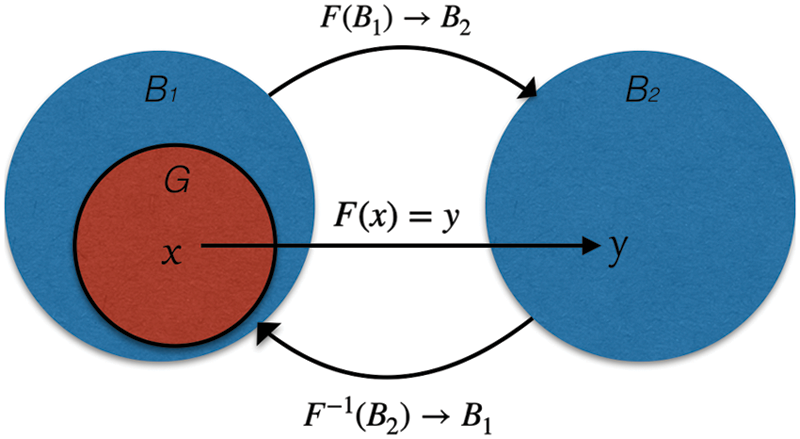
Figure 3: Illustration of classical correctness, see Definition 4

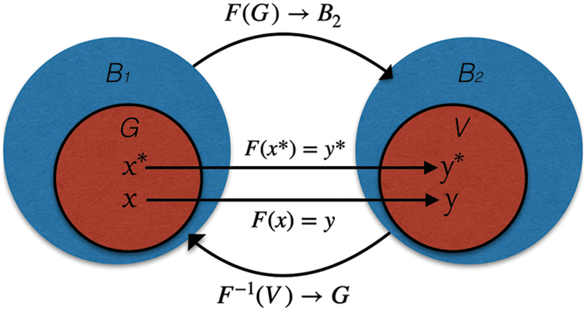
Figure 4: Illustration of conditional correctness, see Definition 5

Definition 2.4 (Classical well-posed problem). Let B1 and B2 be two Banach spaces. Let G⊆B1 be an open set and F:G→B2 be an operator. Consider the equation

F(x)=y,x∈G.(17)

The symbols x and y in this section represent two general variables and are different from the symbols x and y elsewhere in paper. The problem of solution of Eq. (17) is called well-posed by Hadamard, or simply well-posed, or classically well-posed if the following three conditions are satisfied:

1.    For any y∈B2 there exists a solution x=x(y) of Eq. (17) (existence theorem).

2.    This solution is unique (uniqueness theorem).

3.    The solution x(y) depends continuously on y. In other words, the inverse operator F−1:B2→B1 is continuous.

If Eq. (17) does not satisfy to at least one of these three conditions, then the problem (17) is called ill-posed. The problem setting studied in this paper does not satisfy all the above points. Fig. 3 illustrates the definition of classical correctness. Let us now consider the problem (17) when the right hand side is a result of measurements and thus, is given with a noise of level δ. We say that the right hand side of equation

F(x)=y,x∈G.(18)

is given with an error of the level δ>0 (small) if ||y∗−y||B2≤δ, where y∗ is the exact value. The problem (18) can represent the non-regularised form of CPD as well if we associate with x the change point and with y the noisy data corresponding to this change point.

Clearly, if we want to solve the problem (18) with noisy data y, the solution of this problem will be ill-posed in the sense of Hadamard, where our noisy data does not guarantee existence of the solution and makes the operator F−1 not continuous. In order to develop mathematical methods for solution of ill-posed problems Tikhonov has developed regularisation theory starting with the first work on this subject [22]. First, he introduced the definition of a conditionally well-posed problem on the set G.

Definition 2.5 (Conditionally well-posed on the set). Let B1 and B2 be two Banach spaces. Let G⊂B1 be an a priori chosen set of the form G=G¯1, where G1 is an open set in B1. Let F:G→B2 be a continuous operator. Suppose that ||y∗−yδ||B2≤δ. Here y∗ is the ideal noiseless data, yδ is noisy data. The problem (18) is called conditionally well-posed on the set G, or well-posed by Tikhonov on the set G if the following three conditions are satisfied:

1.    It is a priori known that there exists an ideal solution x∗=x∗(y∗)∈G of this problem for the ideal noiseless data y∗.

2.    The operator F:G→B2 is one-to-one.

3.    The inverse operator F−1 is continuous on the set F(G).

Fig. 4 illustrates the definition of conditional correctness. Thus, the concept of Tikhonov’s consists of the following three conditions we should consider when we solve the ill-posed problem with noisy data:

1.    A priori assumption that there exists an ideal exact solution x∗ of Eq. (18) for an ideal noiseless data y∗.

2.    A priori choice of the correctness set G. In other words, we should a priori choose the set of admissible parameters for solution x.

3.    If we want to develop a stable numerical method for the solution of the problem (18), one should:

•   Assume that there exists a family {yδ} of right hand sides of Eq. (18), where δ>0 is the level of the error in the data with ||y∗−yδ||B2≤δ.

•   One should construct a family of approximate solutions {xδ} of Eq. (18), where xδ corresponds to yδ.

•   The family {xδ} should be such that

limδ→0+||xδ−x∗||=0.

In order to satisfy this conception Tikhonov introduced the notion of a regularisation operator for the solution of Eq. (18).

Definition 2.6 (Regularisation operator). Let Rγ:Kδ0(y∗)→G be a continuous operator depending on the regularisation parameter γ>0. The operator Rγ is called the regularisation operator for

F(x)=y(19)

if there exists a function γ(δ) defined for δ∈(0,δ0) such that

limδ→0||Rγ(δ)(yδ)−x∗||B1=0.

Thus, to find approximate solution of the problem (19) with noisy data y, Tikhonov proposed minimise the following regularisation functional Jγ(x),

Jγ(x)=12||F(x)−y||B22+γ2ψ(x),(20)

Jγ:G→R,

where γ=γ(δ)>0 is a small regularisation parameter and γ2ψ(x) is the regularisation term.

There can be a lot of different regularisation procedures for the solution of the same ill-posed problem [23–25], different methods for choosing the regularisation parameter γ [26–30] and a lot of different regularisation terms. Main popular regularisation terms are [26]

•   γ2‖x‖Lpp,1≤p≤2

•   γ2‖x‖TV, TV means total variation, ‖x‖TV=∫G‖∇x‖2dx

•   γ2‖x‖BV, BV means bounded variation, a real-valued function whose TV is bounded (finite).

•   γ2‖x‖H1

•   γ2(‖x‖L1+‖x‖L22)

•   γ2‖x‖H1,2

•   Combination of γ2‖x‖H1 and γ2‖x‖L2

•   Specific choices appearing in analysing of big data using machine learning [13,31].

2.2.4 Regularised Cost Functions

As was discussed in the previous section, by adding a regularisation to Eq. (15) we transform ill-posed CPD with noisy data into conditionally well-posed problem. Thus, we can better handle the noisy data. The regularisation term is dependent on the model parameters β and a regularisation parameter γ, where γ can be estimated or chosen as a constant (γ>0). If γ=0, we get the ordinary linear regression model, presented in Eq. (15). The use of regularisation has been studied widely, where the approach can provide a theoretical, numerical or iterative solution for ill-posed problems [25,27,30]. Tikhonov’s regularisation has been used when solving inverse problems [21,24] and in machine learning for classification and pattern recognition, see details and analysis of different regularisation methods in [13–15,32]. In this work we study Ridge and Lasso regularisation which are standard approaches of Tikhonov regularisation [33,34].

The first regularisation approach which is studied in this work is the Ridge regression,

cRidge(ya:b):=minβ∈Rp∑t=a+1b(yt−(β0+βxt))2+γ∑j=1p||βj||22,(21)

where the regularisation term is the aggregated squared L2-norm of the model coefficients. If the L2-norm is exchanged for the L1-norm we get Lasso regularisation. The cost functions is defined

cLasso(ya:b):=minβ∈Rp∑t=a+1b(yt−(β0+βxt))2+γ∑j=1p|βj|(22)

where γ is the previously described regularisation parameter. Note that this parameter can be the same as the parameter in the Ridge regression (21) but these are not necessarily equal. In all of our computations we empirically set γ=1. The study of how to choose the optimal value for gamma is the topic of future research.

2.3 Bayesian Approach

In contrast to the optimisation approach, the Bayesian approach is based on Bayes’ probability theorem, where the maximum probabilities are identified. It is based on the Bayesian principle of calculating a posterior distribution of a time stamp being a change point, given a prior and a likelihood function. From this posterior distribution, we can identify the points which are most likely to be change points. The upcoming section will briefly go through the theory behind the Bayesian approach. For more details and proofs of the used Theorem, the reader is directed to the work by Fearnhead [12]. The section is formulated as a derivation of the sought after posterior distribution for the change points. Using two probabilistic quantities P and Q, we can rewrite Bayes’ formula to a problem specific formulation which gives the posterior probability of a change point τ. Finally, we combine the individual posterior distribution to get a joint distribution for all possible change points.

In our case, we wish to predict the probability of a change point τ given the data y1:n. The principle behind the Bayesian approach lies in the probabilistic relationship formulated by Bayes in 1763 [35] as

Pr(A|B)=Pr(A,B)Pr(B)=Pr(B|A)Pr(A)Pr(B),(23)

which can be reformulated in terms of CPD problem. A posterior probability distribution for a change point τ given the data can be expressed as

Pr(τ|y1:n)=Pr(τ,y1:n)Pr(y1:n)=Pr(y1:τ|τ)Pr(yτ+1:n|τ)Pr(τ)Pr(y1:n),(24)

where Pr(y1:τ|τ) and Pr(yτ+1:n|τ) are the likelihood of segments before and after the given change point τ, respectively. The prior distribution Pr(τ) indicates the probability of a potential change point τ existing and y1:n represents the entirety of the signal. Using the (MAP) we identify the most probable timestamps of being change points. Expressing MAP(y) in logarithmic terms, we get

maxτ∈[0:n]log⁡Pr(τ|y1:n)=maxτ∈[0:n][log⁡Pr(y1:τ|τ)+log⁡Pr(yτ+1:n|τ)+log⁡Pr(τ)−log⁡Pr(y1:n)].(25)

Similarly to Fearnhead [12], we will define two functions P and Q which are used for calculations in the Bayesian approach. First, we define the probability of a segment P(t,s), given two entries belonging to the same segment

P(t,s)=Pr(yt:s|t,s∈Sj)=∫∏i=tsf(yi|θSj)π(θSj)dθSj,(26)

where f is the probability density function of entry yt belonging to a segment Sj with parameter θSj. We note that this function has similarities used in the optimisation approach, namely in Eq. (5), where we assume a distribution for each segment. In this work, this likelihood will be the Gaussian observation log-likelihood function, but other function choices can be made. Note that π(θSj) is the prior for the parameters of segment Sj. The discrete intervals [t,s],t≤s make P an upper triangular matrix which elements are probabilities for segments yt:s. Note that this probability is independent of the number of true change points K.

The second function, Q, indicates the probability of a final segment yt:n starting at time ti given a change point at previous time step, ti−1. This probability is affected by the number of change points K, and also which of the change points that is located at time ti−1. Since we do not know the exact number of change points K, we use a generic variable k, and perform calculations for all possible values of K. The recurrent function is defined as

Qj(k)(i)=Pr(yi:n|τj=i−1,k)=∑s=in−k+jP(t,s)Qj+1(k)(s+1)πk(τj=i−1|τj+1=s),(27)

Q(k)(1)=Pr(y1:n|k)=∑s=1n−kP(1,s)Q1(k)(s+1),(28)

where Q(k)(1) is the first time step and is a special case of Qj(k)(i). The time index is indicated with i∈[2,…,n]. The assumed number of change points is denoted k∈{1,…,n−1}, where j∈{1,…,k} indicates which of the k assumed change points we are currently at. The prior πk is based on the distance between change points, naturally dependent on k. This prior can be any point process, where the simplest example is the constant prior with probability p=1/n, where n is the number of samples. Other examples include the negative binomial and Poisson distribution. Note that the prior should be a point process since we have discrete time steps. The first time step is defined as an altered function in (28). The result from this recursion is saved in an array of length n. A derivation and proof for this function Q are provided by Fearnhead in Theorem 1 [12]. When calculating the sums in Eqs. (27)–(28), the terms on the right hand side contribute to the function value. We use the same truncation rule as expressed in the work by Fearnhead [12], where ϵ=10−10 is used as a truncation threshold.

Using functions P and Q, the posterior distribution Pr(τj|τj−1,y1:n,k) for change point τj, given the previous change point τj−1, the data y1:n and number of change points, can be calculated. Using Eq. (24) along with the expressions for P and Q, we can formulate the posterior distribution for change point τj as

Pr(τj|τj−1,y1:n,k)==Pr(yτj−1+1:τj|τj−1+1,τj∈Sj)Pr(yτj+1:n|τj,k)πk(τj−1|τj)Pr(yτj−1:n|τj−1,k)=P(τj−1+1,τj)Qj(k)(τj+1)πk(τj−1|τj)Qj−1(k)(τj−1),(29)

where

Pr(τ1|y1:n,k)=P(1,τ1)Q(k)(τ1+1)πk(τ1)Q(k)(1).(30)

Here, πk is the probability of τj based on the distance to τj−1. This posterior distribution indicates the probability of change point τj occurring in each possible time step ti∈[1,n−1]. The formulas in (29) and (30) can be applied for each possible number of change points, where k can range from 1 to n−1. Therefore, this posterior distribution is calculated for every available number of change points k.

The final step in the Bayesian approach is to combine the conditional probabilities for each individual change point (seen in Eq. (29)) to get the joint distribution for all available change points. The joint probability is calculated as

Pr(τ1,τ2,…,τn−1|y1:n)=(∏j=2n−1Pr(τj|τj−1,y1:n,k))Pr(τ1|y1:n,k),(31)

where the first change point τ1 has a different probability formulation due to not having any previous change point. This joint probability can be used to identify the most likely change points. Examples of calculated posterior distributions are found in Appendix A [20], where we see the varying probability of being a change point for each sample in the dataset. A sampling method can be used to draw samples from the joint posterior distribution, where we are interested in the points that are most likely to be change points. This means that we can identify the peaks in the posterior distribution, above a set confidence level. This is explained further in Section 3.2. In our computations, we use the python function find_peaks [36] to identify the posterior distribution’s extreme points (local maximums). These local maximums are taken as the change points.

2.4 Methods of Error Estimation

In this section, the used metrics for evaluating the performance of the CPD algorithms are presented. The metrics has previously been used to compare the performance of change point detection algorithms [7,19], where a selection of metrics has been chosen to cover the general performance. We first differentiate between the true change points and the estimated ones. The true change points are denoted by T∗={τ0∗,…,τK+1∗} while T^={τ^0,…,τ^K+1} indicate estimations. Similarly, the number of true change points is indicated K∗ while K^ represents the number of predicted points.

The most straight forward measure is to compare the number of predictions with the true number of change points. This is know as the Annotation error, and is defined as

AE:=|K^−K∗|,(32)

where K^ is the estimated and K∗ the true change points. This does not indicate how precise the estimations are, but can indicate if the model is over- or under-fitted.

Another similarity metric of interest is the Rand Index (RI) [7]. Compared to the previous distance metrics, the rand index gives the similarity between two segmentations as a percentage of agreement. This metric is commonly used to compare clustering algorithms. To calculate the index, we need to define two additional sets which indicate whether two samples are grouped together by a given segmentation or if they are not grouped together. These sets are defined by Truonga et al. [7] as

GR(T):={(s,t),1≤s<t≤T:sandtbelongtothesamesegmentinT},NGR(T):={(s,t),1≤s<t≤T:sandtbelongtodifferentsegmentsinT},

where T is some segmentation for a time interval [1,T]. Using these definitions, the rand index is calculated as

RI(T^,T∗):=|GR(T^)∩GR(T∗)|+|NGR(T^)∩NGR(T∗)|T(T−1),(33)

which gives the number of agreements divided by possible combinations.

To better understand how well the predictions match the actual change points, one can use the measure called the meantime error which calculates the meantime between each prediction to the closest actual change point. The meantime should also be considered jointly with the dataset because the same magnitude of meantime error can indicate different things in different datasets. For real-life time series data, the meantime error should be recorded in units of time, such as seconds, in order to make the results intuitive for the user to interpret. The meantime is calculated as

MT(T^,T∗)=∑j=1K^minτ∗∈T∗|τj^−τ∗|K^.(34)

A drawback of this measure is that it focuses on the predicted points. If there are fewer predictions than actual change points, the meantime might be lower if the predictions are in proximity of some of the actual change points but not all. Note that the meantime is calculated from the prediction and does not necessarily map the prediction to corresponding true change point, only the closest one.

Two of the most common metrics of accuracy in predictions are precision and recall. These metrics give a percentage of how well the predictions reflect the true values. The precision metric is the fraction of correctly identified predictions over the total number of predictions, while the recall metric compares the number of identified true change points over the total number of true change points. These metrics can be expressed as

precision=|TP(T^,T∗)||T|^,recall=|TP(T^,T∗)||T∗|,(35)

where TP represents the number of true positives between the estimations T^ and true change points T∗. Mathematically, TP is defined as TP(T^,T∗)={τ∗∈T∗|τ^∈T^:|τ∗−τ^|<ϵ}, where ϵ is some chosen threshold. The threshold gives the radius of acceptance, meaning the acceptable number of time steps which can differ between prediction and true value. The two metrics (35) can be incorporated into a combined metric, known as the F-score. The metric F1-score uses the harmonic mean of the precision and recall and is applied in this work. As reviewed in this section, the metrics measure the similarity between the predicted change points and the actual change points from various perspectives. Hence this work adopt all of them to give a comprehensive evaluation of the performance of CPD algorithms.

3  Results

This section presents numerical examples illustrating the performance comparison of methods discussed in the paper. First, we describe the real-life dataset together with testing procedure. Next, several numerical examples demonstrate performance of CPD methods.

3.1 PRONTO Dataset

Multiphase flow processes are frequently seen in industries, when two or more substances, such as water, air and oil, are mixed or interact with each other. Different flow rates of the multiphase flows and different ratios between these flows will result in different flow regimes and the process is hence operated in different operating modes. An example is the PRONTO benchmark dataset, available via Zendo [37], and an illustration of the facility is seen in Fig. 5. The dataset is collected from a multiphase flow rig. In the described process, air and water are pressurised respectively, where the pressurised mix travels upwards to a separator located at an altitude. A detailed description of the process can be found in [38].

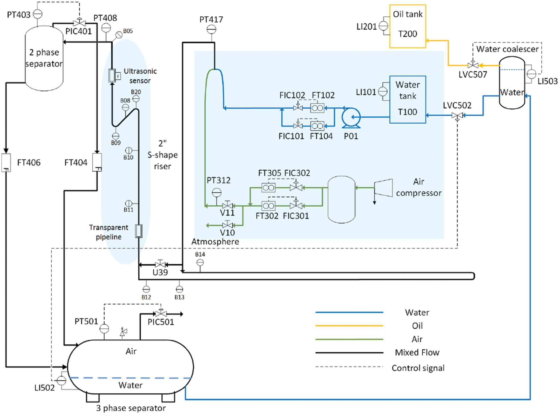
Figure 5: Illustration of the multi-flow facility for generating the PRONTO dataset [38]. The shaded areas indicate the air and water flows that are studied in this paper

Since the varying flow rates can result in varying flow regimes, we focus on the process variables of the flow rates. The signals are sampled with the same sampling rate and can be examined simultaneously, but will be treated individually in this work. The CPD approaches are applied to four process variables, including two flow rates of the inlet air denoted by Air In 1, Air In 2 and two flow rates of the inlet water represented as Water In 1 and Water In 2, visualised in Fig. 6. The figure shows these four signals, where the different operating modes are marked with alternating grey shades in the background.

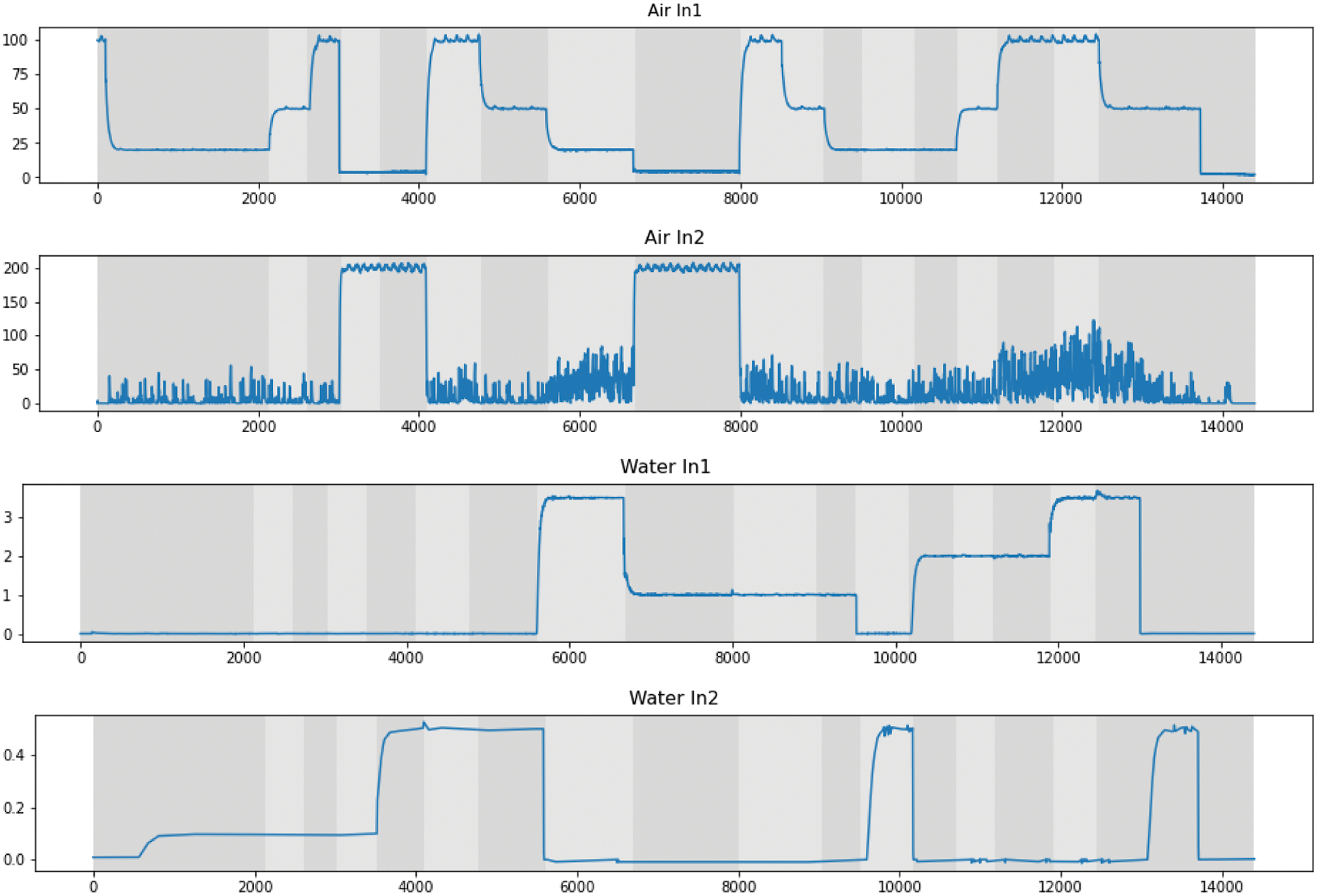
Figure 6: The process variables Air In 1, Air In 2, Water In 1 and Water In 2 described in [38]. The segments of different operating modes are indicated with alternating grey regions, and sixteen change points are present on the boarder between segments

We take these changes in the operating mode as the true change points and they are used for evaluating the CPD algorithms. The operating modes were recorded during the experiment and always corresponded to the change in the water and air flow rates. However, due to human errors some change points were missing at the end of the experiment (after around the 13,000-th sample).

We observe a range of typical behaviours in the time series data, such as piecewise constant segments, exponential decay and change in variance. One can see that the changes in the flow rates will result in the changes in the operating mode. On the other hand, such changes in operating mode may not always be recorded during the process operation and then not always available for process data analysis. Therefore, the change points in the data will be a good indicator of changes in the operating mode if the CPD approaches can detect the change points accurately.

3.2 Testing Procedure

Both CPD approaches introduced in Section 2 are tested on the PRONTO dataset. To make predictions with the Python package RUPTURES [39], first one needs to specify the algorithm with search direction and cost function. In addition to this, the penalty level should also to be specified. The value of the perfect penalty β in Eq. (1) is not known a priori, therefore, multiple predictions are done for various penalty values β∈N∪{0}. If β=0 the algorithm receives no penalty when adding a change point, and the algorithm can add as many change points as necessary to minimise the cost functions. Predictions are made using all cost functions, where both PELT and WIN are used, and the time stamps of the detected change points are saved.

Using the concepts derived in Section 2.3 we can calculate posterior distribution with probabilities for each time step being a change point. Due to the algorithm being computationally heavy, the resolution of the data is reduced in the real dataset by PRONTO using Piecewise Aggregate Approximation (PAA) [40]. The function aggregates the values of a window to an average value. The used window size is 20 samples. Generally, to conclude a posterior distribution, sampling is used to create a collection of time stamps which in this case represents the change points. In essence, we want to create a sample of the most probable change points, without unnecessary duplicates. To draw this type of samples of change points from the posterior distribution, the function find_peaks in the Python package SciPy [36] is used. The function identifies the peaks in a dataset using two parameters: threshold which the peak value should exceed, and distance which indicates the minimum distance between peaks. The threshold is set to 0.2, where we require a certainty level of at least 20%. The distance is set to 10 time steps to prevent duplicate values. We note that this is not necessarily a proper sampling methodology, and other approaches can be used instead. An alternative sampling method is provided in Fearnhead [12].

All signals are normalised and handled individually such that CPD is applied to each variable for searching change points in univariate signals and the relation between the variables is neglected. The change points are then aggregated to get the combined change points on the entire dataset. The detected change points are compared against the real changes in the operating modes. The metrics provided in Section 2.4 are calculated and saved for each prediction. When enough tests have been performed in terms of penalty values, the results are saved to an external file. The values of the metrics are used to select the best prediction of change points. Our goal is to minimise the annotation error and meantime, and at the same time maximise the F1-score and the rand index.

3.3 Numerical Results

Given the different search directions and cost functions presented in Sections 2.2.1 and 2.2.2, respectively, we can presume that different setups will identify different features and hence differ in predicting of change points. We can also assume that the Bayesian approach, presented in Section 2.3, will not necessarily give the same predictions as the optimisation approach. We note that all algorithms predict the intermediate change points T={τ1,…,τK} along with one artificial change point τK+1:=n. This artificial change point is based on definition and is used when the predictions are compared with respect to created segments, an example being RandIndex. This section presents the results of the two approaches on the real-world dataset.

The result of change point detection by CPD approaches is visualised in Fig. 7. The figure also visualises the time series data from four process signals and the real operating modes. The cost functions are selected to represent the different types of cost functions; maximum likelihood, linear regression and the introduced regularised cost functions. Table 1 shows the predictions obtained using WIN. To calculate the precision and recall, the margin 1% of the number of samples are used, equivalent to 144 s in error is accepted as an accurate indication. The cost functions cNormal and cLasso predict 17 change points and have the lowest absolute error, where these algorithms also have the highest meantime. The smallest meantime is obtained by cL2 and cL1, which predict fewer points. The cost functions cL2 and cL1 have the highest F1-scores of 59.3% and 64.1% respectively and rand index of 96.4% and 97.2%, respectively. The highest precision is obtained using cL2 while the recall is lower at 50%. In the top image of Fig. 7 we see a comparison of the predictions made by cL1, cAR and cRidge. We see similarities in the predictions made by cL1 and cRidge and other predictions made by cAR. We can also note that, due to the linear model structure chosen for the cost function, some algorithms detect two change points when an exponential trend appears; one change point is in the steep part and the other when the trend stabilises. An example can be seen around the 10k-th sample in Fig. 6.

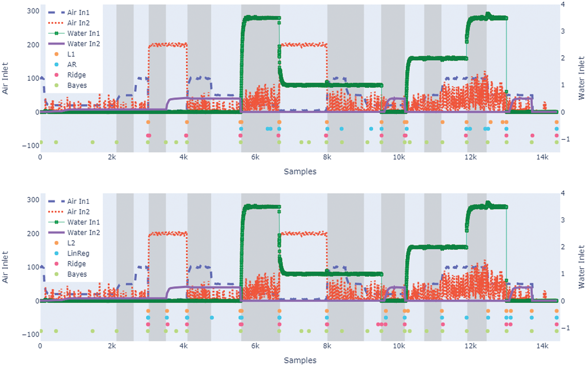
Figure 7: Results for the PRONTO dataset, using various cost functions. The different operating modes are visualised in the background as shaded intervals. Predicted change points are seen in coloured points, which are time points and do not have a value

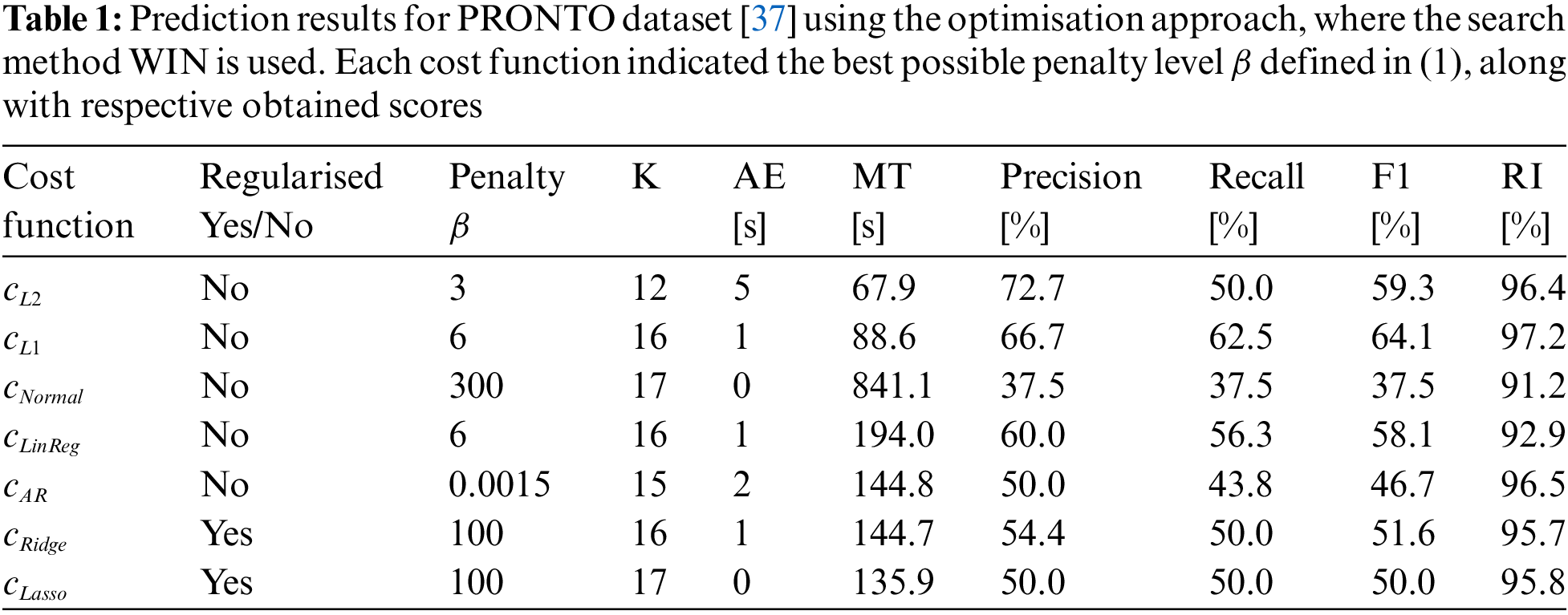
In the bottom image, we see predictions made by cL2, cAR and cRidge when PELT is used. The predictions’ evaluation metrics are given in Table 2. We can note the generally high rand indices and F1-scores, with the exception of cNormal. Most cost functions predict 17 change points, and have a lower meantime compared to the values in Table 1. The smallest meantime of 95.8 time steps is obtained by cAR and the largest meantime by cNormal. The highest F1-score of 66.7% and rand index of 95.4% is obtained by cRidge. In the bottom image of Fig. 7 we see that cL2, cLinReg and cRidge give similar predictions and correspond to many of the true change points.

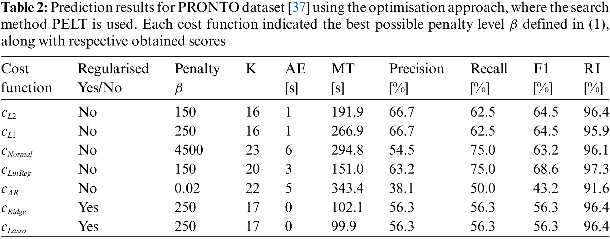
Fig. 7 also shows predictions obtained by the Bayesian method. The method predicts 21 change points, which gives an absolute error AE=4. The meantime of the predictions is 448.9 s. The precision and recall are 65.0% and 81.3%, respectively, which gives an F1-score of 72.2%. The rand index is 96.0%.

4  Discussion and Future Work

In the previous sections, the two CPD approaches are reviewed and applied to the PRONTO benchmark dataset and the detected change points are compared against the real changes in the dataset. We have demonstrated that CPD can be executed on real life data to generate useful insights that may facilitate the analysis. In this section, the results and the implication are discussed and several potential directions are given towards further development and application of CPD for process data analytics.

A natural extension of the work is to conduct the study with other search methods for the optimisation approach and the study can be conducted with other search methods for the optimisation approach and other CPD algorithms to be used as benchmarks. For example, more results on numerically simulated datasets can be found in [20]. When the change points have been identified, the corresponding timestamps can be used to create segments in the data. The segments can correspond to phases in the process, which in turn can be relevant to compare to detect variations in the process phases. Alternatively, change points can indicate anomalies in the process variable signals. This underlines the usability of change point detection in terms of data processing.

Datasets tend to increase in size, and a relevant topic is the suitability for large amounts of data. The two approaches studied in the present work are suitable for datasets with different sizes. The optimisation approach can employ various combinations of cost functions and search directions and the search direction is the major impact factor for the computational complexity. This paper studied two search directions, where the optimal search direction PELT generally gives more accurate predictions. The approximate search direction has a lower computational complexity and can handle larger datasets in a reasonable amount of time. The window size for the WIN algorithm is a tuning parameter that needs to be adjusted accordingly; hence it requires further investigation. On the other hand, the PELT algorithm is computationally heavy, and accurate concerning search direction. Therefore, additional steps, such as down sampling the data, may be necessary when applying PELT to large datasets. The Bayesian approach is also computationally heavy since the posterior distribution needs to be calculated for every time stamp. Nevertheless, the posterior distribution used for identifying the change points only needs to be calculated once and multiple samples of change points can be drawn from the distribution. To conclude, the two CPD approaches may perform differently on larger datasets while having their own merits.

Real data generally have noise, which can affect the predicted change points. For the optimisation approach, some of the common cost functions tend to be sensitive to noise, while the proposed regularised cost functions are less sensitive. It is also noted that the model based cost functions are more sensitive to changes in the shape of the signal than to changes in the values, making model based cost functions more generalisable and less sensitive to noise. Similarly, the Bayesian approach is not too sensitive to noise and can handle value changes in a similar way as the model based cost functions. This indicates that both approaches are compatible with real-world datasets and the optimisation approach demands a suitable cost function to make accurate predictions. Some segments in the PRONTO dataset follow an exponential decay, where some cost functions give indicate two change points in these segments, one at the start of the decay and one where the decay has subsided. In this dataset, we see a change point at the beginning of the exponential decay and not when it has subsided. It is important to select a cost function that handles these segments appropriately to give accurate predictions.

In industrial practice, process experts are often able to provide useful feedback and insights about the operating status of a process. Hence a future direction of applying CPD to process data analytics will be to incorporate the feedback of process experts. For example, it may be interesting to incorporate such information as the prior for the Bayesian approach. This paper has not studied the possibility of user interaction, but suggests it as a topic for future work.

5  Summary

This paper demonstrated how change point detection is relevant for analysing process data, particularly, when the operating condition in the process varies a lot and the corresponding labels are unavailable. Two unsupervised algorithms for change point detection, namely the optimisation approach and the Bayesian approach, are studied and applied to a real-life benchmark dataset. We also illustrated why the optimisation problem of CPD is an ill-posed problem when there is noise in the data and proposed a new type of cost function, using Tikhonov regularisation, for the optimisation approach. Based on the results of the real-life dataset, the paper investigated how the features influence the performance of CPD approaches in the data. The results of CPD on the dataset verified that CPD can detect change points that correspond to the changes in the process and these change points can be considered as labels for data segmentation for further analysis. The proposed regularised cost functions were compared against non-regularised cost functions. It has been shown that, when applied to the real-life dataset with noise, regularised cost functions can achieve better performance of CPD than non-regularised cost functions.

Acknowledgement: The authors acknowledge the financial support by the Federal Ministry for Economic Affairs and Climate Action of Germany (BMWK) within the Innovation Platform “KEEN-Artificial Intelligence Incubator Laboratory in the Process Industry” (Grant No. 01MK20014T). The research of L.B. is supported by the Swedish Research Council Grant VR 2018–03661.

Conflicts of Interest: The authors declare that they have no conflicts of interest to report regarding the present study.

1If f(x∗)≤f(x) or f(x∗)≥f(x) for all x in X within distance ϵ of x∗, then x∗ is a local extreme point.

References

 1.  Duarte, B. P., Saraiva, P. M. (2003). Change point detection for quality monitoring of chemical processes. Computer Aided Chemical Engineering, 14, 401–406. DOI 10.1016/S1570-7946(03)80148-7. [Google Scholar] [CrossRef]

 2.  Eriksson, M. (2019). Change point detection with applications to wireless sensor networks (Ph.D. Thesis). Uppsala University, Sweden. [Google Scholar]

 3.  Lavielle, M., Teyssière, G. (2007). Adaptive detection of multiple change-points in asset price volatility. In: Long-memory in economics, pp. 129–156. Berlin, Heidelberg: Springer Berlin Heidelberg. DOI: 10.1007/978-3-540-34625-8_5. [Google Scholar] [CrossRef]

 4.  Lung-Yut-Fong, A., Levy-Leduc, C., Cappe, O. (2012). Distributed detection of change-points in high-dimensional network trafic data. Statistics and Computing, 22, 485–496. DOI 10.1007/s11222-011-9240-5. [Google Scholar] [CrossRef]

 5.  Page, E. (1954). Continuous inspection schemes. Biometrika, 41(1–2), 100–115. [Google Scholar]

 6.  Page, E. (1955). A test for a change in a parameter occurring at an unknown point. Biometrika, 42(3–4). [Google Scholar]

 7.  Truong, C., Oudre, L., Vayatis, N. (2020). Selective review of offline change point detection methods. Signal Processing, 167, 107299. DOI 10.1016/j.sigpro.2019.107299. [Google Scholar] [CrossRef]

 8.  Basseville, M., Nikiforov, I. (1993). Detection of abrupt changes: Theory and application. Englewood Cliffs: Prentice Hall. [Google Scholar]

 9.  Namoano, B., Starr, A., Emmanouilidis, C., Cristobal, R. (2019). Online change detection techniques in time series: An overview. 2019 IEEE International Conference on Prognostics and Health Management (ICPHM), San Francisco, CA, USA. DOI 10.1109/ICPHM.2019.8819394. [Google Scholar] [CrossRef]

10. Shvetsov, N., Buzun, N., Dylov, D. V. (2020). Unsupervised non-parametric change point detection in electrocardiography. SSDBM 2020. New York, NY, USA: Association for Computing Machinery. DOI 10.1145/3400903.3400917. [Google Scholar] [CrossRef]

11. Harchaoui, Z., Vallet, F., Lung-Yut-Fong, A., Cappe, O. (2009). A regularized kernel-based approach to unsupervised audio segmentation. International Conference on Acoustics, Speech and Signal Processing (ICASSP), pp. 1665–1668. Taipei, Taiwan. [Google Scholar]

12. Fearnhead, P. (2006). Exact and efficient Bayesian inference for multiple changepoint problems. Statistics and Computing, 16, 203–213. DOI 10.1007/s11222-006-8450-8. [Google Scholar] [CrossRef]

13. Bishop, C. M. (2009). Pattern recognition and machine learning. New York: Springer. [Google Scholar]

14. Goodfellow, I., Bengio, Y., Courville, A. (2016). Deep learning. Cambrigde, MA, USA: MIT Press. http://www.deeplearningbook.org. [Google Scholar]

15. Kotsiantis, S. B. (2007). Supervised machine learning: A review of classification techniques. Informatica, 31, 249–268. [Google Scholar]

16. van den Burg, G., Williams, C. (2020). An evaluation of change point detection algorithms. arXiv preprint. DOI 10.48550/arXiv.2003.06222. [Google Scholar] [CrossRef]

17. Mirko, B. (2011). Contrast and change mining. WIREs Data Mining and Knowledge Discovery, 1(3), 215–230. DOI 10.1002/widm.27. [Google Scholar] [CrossRef]

18. Hido, S., Idé, T., Kashima, H., Kubo, H., Matsuzawa, H. (2008). Unsupervised change analysis using supervised learning. Advances in knowledge discovery and data mining. Berlin, Heidelberg: Springer Berlin Heidelberg. [Google Scholar]

19. Aminikhanghahi, S., Cook, D. (2017). A survey of methods for time series change point detection. Knowledge and Information Systems, 51, 339–367. DOI 10.1007/s10115-016-0987-z. [Google Scholar] [CrossRef]

20. Gedda, R. (2021). Interactive change point detection approaches in time-series (Master’s Thesis). Göteborg, Sweden: Chalmers University of Technology. https://hdl.handle.net/20.500.12380/302356. [Google Scholar]

21. Beilina, L., Klibanov, M. (2012). Approximate global convergence and adaptivity for coefficient inverse problems. London: Springer. [Google Scholar]

22. Tikhonov, A. (1943). On the stability of inverse problems. Doklady of the USSR Academy of Science, 39, 195–198. [Google Scholar]

23. Bakushinskiy, A., Kokurin, M., Smirnova, A. (2011). Iterative methods for Ill-posed problems: An introduction. Berlin, New York, USA: de Gruyter. DOI 10.1515/9783110250657. [Google Scholar] [CrossRef]

24. Bakushinsky, A. B., Kokurin, M. Y. (2004). Iterative methods for approximate solution of inverse problems. Dordrecht, Netherlands: Springer. [Google Scholar]

25. Tikhonov, A., Arsenin, V. (1977). Solutions of ill-posed problems. Hoboken, USA: Wiley. https://www.researchgate.net publication/256476410_Solution_of_Ill-Posed_Problem. [Google Scholar]

26. Ito, K., Jin, B. (2015). Inverse problems: Tikhonov theory and algorithms. In: Series on applied mathematics, vol. 22, pp. 32–45. Singapore: World Scientific. [Google Scholar]

27. Kaltenbacher, B., Neubauer, A., Scherzer, O. (2008). Iterative regularization methods for nonlinear Ill-posed problems, pp. 64–71. Berlin, New York, USA: De Gruyter. https://doi.org/10.1515/9783110208276.64 [Google Scholar]

28. Lazarov, R., Lu, S., Pereverzev, S. (2007). On the balancing principle for some problems of numerical analysis. Numerische Mathematik, 106, 659–689. DOI 10.1007/s00211-007-0076-z. [Google Scholar] [CrossRef]

29. Morozov, V. (1966). On the solution of functional equations by the method of regularization. Doklady Mathematics, 7, 414–417. [Google Scholar]

30. Tikhonov, A., Goncharsky, A., Stepanov, V., Yagola, A. (1995). Numerical methods for the solution of ill-posed problems. Netherlands: Springer. [Google Scholar]

31. Zickert, G. (2020). Analytic and data-driven methods for 3D electron microscopy (Ph.D. Thesis). Sweden: KTH Royal Institute of Technology, Stockholm. http://urn.kb.se/resolve?urn=urn:nbn:se:kth:diva-281931. [Google Scholar]

32. Beilina, L. (2020). Numerical analysis of least squares and perceptron learning for classification problems. Open Journal of Discrete Applied Mathematics, 3, 30–49. DOI 10.30538/psrp-odam2020.0035. [Google Scholar] [CrossRef]

33. Ivezić, ž, Connolly, A., der Plas, J. V., Gray, A. (2014). Statistics, data mining, and machine learning in astronomy: A practical python guide for the analysis of survey data. Princeton Series in Modern Observational Astronomy. Princeton: Princeton University Press. https://books.google.de/books?id=h2eYDwAAQBAJ. [Google Scholar]

34. Saleh, A., Arashi, M., Kibria, B. (2019). Theory of ridge regression estimation with applications. USA: Wiley. https://books.google.de/books?id=v0KCDwAAQBAJ. [Google Scholar]

35. Bayes, T. (1763). An essay toward solving a problem in the doctrine of chances. Philosophical Transactions, 8, 157–71. DOI 10.1098/rstl.1763.0053. [Google Scholar] [CrossRef]

36. Virtanen, P., Gommers, R., Oliphant, T. E., Haberland, M., Reddy, T. et al. (2020). SciPy 1.0: Fundamental algorithms for scientific computing in Python. Nature Methods, 17, 261–272. DOI 10.1038/s41592-019-0686-2. [Google Scholar]

37. Stief, A., Tan, R., Cao, Y., Ottewill, J. (2019). PRONTO heterogeneous benchmark dataset. Zenodo. DOI 10.5281/zenodo.1341583. [Google Scholar] [CrossRef]

38. Stief, A., Tan, R., Cao, Y., Ottewill, J., Thornhill, N. et al. (2019). A heterogeneous benchmark dataset for data analytics: Multiphase flow facility case study. Journal of Process Control, 79, 41–55. DOI 10.1016/j.jprocont.2019.04.009. [Google Scholar] [CrossRef]

39. Truong, C. (2020). Ruptures. https://github.com/deepcharles/ruptures. [Google Scholar]

40. Tavennard, R. (2018). Tslearn piecewise_aggregate_pproximation (PAA). https://tslearn.readthedocs.io/en/stable/gen_modules/piecewise/tslearn.piecewise.PiecewiseAggregateApproximation.html. [Google Scholar]