A Study of Traveling Wave Structures and Numerical Investigation of Two-Dimensional Riemann Problems with Their Stability and Accuracy

1  Introduction

Diverse phenomena in nature and technology are described using nonlinear evolution equations (NLEEs). In physics, for instance, the heat transfer and the traveling wave phenomena are successfully modeled by PDEs. In chemistry, the dispersion of a chemically reactive substance is controlled by PDEs. Also, PDEs are invoked to characterize population growth problems. Moreover, most physical incidents of shallow-water waves, quantum mechanics, plasma physics, electricity, fluid dynamics, and more others are investigated using PDEs. In order to better comprehend the qualitative characteristics of such equations, one can study their analytical solutions. A distinct range of traveling wave structures allows us to explain the mechanisms of immense complicated phenomena. As a result, some researchers have revealed numerous effective methods. Some of the powerful approaches are the Sine-Gordon expansion approach [1], the modified simple equation technique [2], the tanh-sech process [3,4], the trial equation method [5], the exp(−f(ζ))-expansion principal [6,7] and the generalized exponential rational function approach [8]. More methods can be easily seen in references [9–15].

The Riemann wave system [16,17] is given by

Vt+αΓxyy+βΓVy+γUVx=0,Vy=Ux,Vx=Γy,(1)

where α,β and γ are constants. System (1) describes a (2+1)-dimensional interaction for the propagation of Riemann waves in the x-axis and y-axis. The Riemann wave equations have been investigated by some scientists using various methods. For example, Shao [18] examined the stability of the solution of the quasi-linear hyperbolic systems under the influence of some BV perturbations. Shao [19] presented several solutions with satisfying some conditions. Chen et al. [20] used the generalized expansion approach of the Riccati equation to extract some soliton-like solutions for Eq. (1) when m=n=4b, where b is a constant. The modified mapping principle was applied in [21] to establish a class of periodic wave solutions in terms of the Jacobi elliptic functions. Moreover, Abdelrahman et al. [22] utilized the singular manifold technique to construct two general solutions for system (1). Every obtained solution contains two arbitrary functions. Then, some periodic wave solutions were derived from the obtained general solutions. In [16], the tanh method was implemented to generate some traveling wave solutions for Eq. (1). The generalized Kudryashov approach was applied in [17] to systematically and graphically show the traveling wave solutions of Eq. (1). While, in this paper, we present analytical and numerical solutions to Eq. (1) using the generalized exponential rational function approach [8] and finite difference methods, respectively.

Since our knowledge of constructing exact solutions for the Riemann wave equations is basically based on few techniques, we utilize the generalized exponential rational function approach [8] to construct the exact solutions of the considered equations. This technique depends on Jacobi elliptic functions. As a result, various solitary traveling wave solutions can be simply generated in terms of trigonometric and hyperbolic functions. Regarding the numerical solution, some numerical simulations are presented using the finite difference method to emphasize that the obtained results are accurate. The numerical solutions of the considered system are obtained by approaching the equations on a mesh using the finite-difference notations. The domain is divided into a limited set of grids to achieve meshes for both independent variables x and y. It is well known that the wave of the solutions has areas with rapid spatial changes, for instance, steep fronts structures. In order to resolve these types of areas, fine numbers of grids, for x and y, are required. The step size, Δx=xi−xi−1, Δy=yi−yi−1 should be extremely small to catch these regions. Computationally, it is intensive and expensive. Hence, I strive to achieve an alternative discretizing for the meshes to have a non-uniform mesh that manually sets more grids in where the solution varies rapidly and fewer grids outside these regions. And then, I used the stiff ODE solver DASPK [23] to solve the obtained ODEs of the semi-discretization of the system. This ODEs solver is an implicit iterative method, based on the Krylov subspace method. They are applied to solve the system of linearized equations. They also allow converting the Jacobian matrix to be LU factorized to make the calculations faster. I additionally studied, here, the stability and the error analysis for the numerical schemes.

2  Methodology

The generalized exponential rational function approach is comprehensively summarized in this section, as presented in [8]. Assume that

P(V,Vx,Vt,Vxx,Vxy,Vxxy,U,Ux,Uy,Γ,Γx,Γy,…)=0,(2)

is a given nonlinear PDE in the unknown functions V=V(x,y,t),U=U(x,y,t) and Γ=Γ(x,y,t). P is a polynomial in V,U and Γ and their partial derivatives. Suppose that ζ=μx+δy−wt, where μ,δ and w are unknown parameters that will be computed later. Thus,

V(x,y,t)=v(ζ),U(x,y,t)=u(ζ),Γ(x,y,t)=ψ(ζ).(3)

Then, Eq. (2) is converted into

Q(v,v′,v′′,v′′′,u,u′,ψ,ψ′,…)=0,(4)

where ^{\prime}=ddζ. According to the proposed method, the formal solution of Eq. (4) is written as

Υ(ζ)=p1exp⁡(q1ζ)+p2exp⁡(q2ζ)p5exp⁡(q3ζ)+p6exp⁡(q4ζ),(5)

where p1p2,p5,p6,q1,q2,q3, and q4 are complex (or real) constants so that Eq. (2) is expressed as

v(ζ)=A0+∑k=1NAkΥ(ζ)k+∑k=1NBkΥ(ζ)−k,(6)

The balance principle is used to determine the value of N appearing in Eq. (6). Moreover, the coefficients A0,Ak and Bk(k=1,2,…,N) is evaluated such that Eq. (6) satisfies Eq. (4). Inserting Eq. (6) into Eq. (4) gives a polynomial from which one can obtain an algebraic system solved using Mathematica or Maple. The values of the above-mentioned constants are included in the solutions of this system. Substituting these values into Eq. (6) yields the exact solutions of Eq. (2).

3  Traveling Wave Solution

In this section, we study the exact solutions of system (1) using the generalized exponential rational function approach. Substitute Eq. (3) into system (1) to have

−wvζ+μδ2αψζζζ+βδψvζ+γμuvζ=0,uζ=δμvζ,ψζ=μδvζ.(7)

We now integrate each equation in system (7) with respect to ζ to obtain

−wv+b0vζζ+B1v2=0,u=δμv,ψ=μδv,(8)

where b0=αμ2δ and B1=0.5δ(β+γ). Balancing the highest order of vζζ with the nonlinear term v2 in system (8) evaluates the value of N given by N=2. As a result, the exact solutions are shown as follows:

v(ζ)=A0+A1Υ(ζ)+A2Υ(ζ)2+B1Υ(ζ)−1+B2Υ(ζ)−2,u(ζ)=δμv(ζ),ψ(ζ)=μδv(ζ),(9)

where Υ(ζ) is presented in Eq. (5). We insert systems (9) into (8) to obtain the traveling wave solutions of (1) which are written as follows.

Family 1: For p=[1,−1,1,1] and q=[−1,1,−1,1], Eq. (5) becomes

Υ(ζ)=−tanh⁡(ζ).(10)

Substituting Eq. (10) into the first equation of system (9) and then we insert the result into the first equation of system (8) give an algebraic system whose solutions are given as follows:

Case 1:

A0=−A2,A1=B1=B2=0,μ=±−A2β−A2γ23α,δ=−μ,w=−13A2δ(β+γ).(11)

Substituting Eq. (11) into system (9) and Eq. (10) gives the exact solutions of system (1) which are illustrated as follows:

V1(x,y,t)=−A2+A2tanh2(±−A2β−A2γ23αx+δy+13A2δ(β+γ)t),U1(x,y,t)=±2δ3α−A2β−A2γV(x,y,t),Γ1(x,y,t)=±−A2β−A2γ2δ3αV(x,y,t).(12)

Case 2:

A0=−13A2,A1=B1=B2=0,μ=±−A2β−A2γ23α,δ=−μ,w=13A2δ(β+γ).(13)

Inserting Eq. (13) into system (9) and Eq. (10) yields the exact solutions of system (1) which are expressed as

V2(x,y,t)=−13A2+A2tanh2(±−A2β−A2γ23αx+δy−13A2δ(β+γ)t),U2(x,y,t)=±2δ3α−A2β−A2γV(x,y,t),Γ2(x,y,t)=±−A2β−A2γ2δ3αV(x,y,t).(14)

Case 3:

A0=−2A2,A1=B1=0,B2=A2,μ=±−A2β−A2γ23α,δ=−μ,w=−43A2δ(β+γ).(15)

Plugging Eq. (15) into system (9) and Eq. (10) gives the traveling wave solutions of system (1) which are given by

V3(x,y,t)=−2A2+A2tanh2(±−A2β−A2γ23αx+δy+43A2δ(β+γ)t)+A2coth2(±−A2β−A2γ23αx+δy−43A2δ(β+γ)t),U3(x,y,t)=±2δ3α−A2β−A2γV(x,y,t),Γ3(x,y,t)=±−A2β−A2γ2δ3αV(x,y,t).(16)

Case 4:

A0=−23A2,A1=B1=0,B2=A2,μ=±−A2β−A2γ23α,δ=−μ,w=43A2δ(β+γ).(17)

Putting Eq. (11) into system (9) and Eq. (10) leads to the exact solutions of system (1) which are shown as

V4(x,y,t)=−23A2+A2tanh2(±−A2β−A2γ23αx+δy−43A2δ(β+γ)t)+A2coth2(±−A2β−A2γ23αx+δy−43A2δ(β+γ)t),U4(x,y,t)=±2δ3α−A2β−A2γV(x,y,t),Γ4(x,y,t)=±−A2β−A2γ2δ3αV(x,y,t).(18)

Family 2: For p=[i,−i,1,1] and q=[i,−i,i,−i], Eq. (5) becomes

Υ(ζ)=−sin⁡ζcos⁡ζ,(19)

Case 1:

A0=13A2,A1=B1=B2=0,μ=±−A2β−A2γ23α,δ=−μ,w=−13A2δ(β+γ).(20)

Substituting Eq. (20) into system (9) and Eq. (19) gives the exact solutions of system (1) which are shows as follows:

V5(x,y,t)=13A2+A2sin2(±−A2β−A2γ23αx+δy+13A2δ(β+γ)t)cos2(±−A2β−A2γ23αx+δy+13A2δ(β+γ)t),U5(x,y,t)=±2δ3α−A2β−A2γV(x,y,t),Γ5(x,y,t)=±−A2β−A2γ2δ3αV(x,y,t).(21)

Case 2:

A0=A2,A1=B1=B2=0,μ=±−A2β−A2γ23α,δ=−μ,w=13A2δ(β+γ).(22)

Inserting Eq. (22) into system (9) and Eq. (19) yields the traveling wave solutions of system (1) which are

V6(x,y,t)=A2+A2sin2(±−A2β−A2γ23αx+δy+13A2δ(β+γ)t)cos2(±−A2β−A2γ23αx+δy+13A2δ(β+γ)t),U6(x,y,t)=±2δ3α−A2β−A2γV(x,y,t),Γ6(x,y,t)=±−A2β−A2γ2δ3αV(x,y,t).(23)

Case 3:

A0=2A2,A1=B1=0,B2=A2,μ=±−A2β−A2γ23α,δ=−μ,w=43A2δ(β+γ).(24)

Putting Eq. (24) into system (9) and Eq. (19) gives the exact solutions of system (1) which are

V7(x,y,t)=2A2+A2sin2(±−A2β−A2γ23αx+δy+13A2δ(β+γ)t)cos2(±−A2β−A2γ23αx+δy+13A2δ(β+γ)t),+A2cos2(±−A2β−A2γ23αx+δy+13A2δ(β+γ)t)sin2(±−A2β−A2γ23αx+δy+13A2δ(β+γ)t),U7(x,y,t)=±2δ3α−A2β−A2γV(x,y,t),Γ7(x,y,t)=±−A2β−A2γ2δ3αV(x,y,t).(25)

Case 4:

A0=−23A2,A1=B1=0,B2=A2,μ=±−A2β−A2γ23α,δ=−μ,w=−43A2δ(β+γ).(26)

Substituting Eq. (26) into system (9) and Eq. (19) leads to the exact solutions of system (1) which are expressed as

V8(x,y,t)=−23A2+A2sin2(±−A2β−A2γ23αx+δy+13A2δ(β+γ)t)cos2(±−A2β−A2γ23αx+δy+13A2δ(β+γ)t),+A2cos2(±−A2β−A2γ23αx+δy+13A2δ(β+γ)t)sin2(±−A2β−A2γ23αx+δy+13A2δ(β+γ)t),U8(x,y,t)=±2δ3α−A2β−A2γV(x,y,t),Γ8(x,y,t)=±−A2β−A2γ2δ3αV(x,y,t).(27)

4  Stability of the Analytical Solution

We introduce the Hamiltonian system in this section. Hamiltonian system is applied on analytical solutions to test their stability on a specific interval. The Hamiltonian system [24,25] is expressed by

Π(w)=∫−∞∞12v2(ζ)dζ,(28)

where Π indicates the momentum function. Furthermore, w presents the wave speed and v(ζ) is the considered analytical solution. The sufficient condition for the stability is

∂Π∂w>0.(29)

When we apply Eqs. (28) and (29) on Eq. (18) over the rectangular domain [−20,40]×[0,1], we obtain

∂Π∂w=18.24>0,(30)

where the parameters A2=1.2,β=−0.5,α=2.70, and γ=−2.20. As a result, the analytical solutions are unconditionally stable.

5  Finite Difference Semi-Discretization Scheme on a Fixed Mesh

This section is devoted to study the numerical solutions of system (1) over the physical domain [a,b]×[c,d], where a and b indicate the boundary of the domain in x direction. Moreover, c and d indicate the boundary of the domain in y direction and Te denotes a specific time. The central finite differences are utilized to establish the numerical schemes of this system. We firstly split the domain [a,b]×[c,d] into (N+1)×(M+1) discrete points as follows:

xn=a+nΔx,n=0,1,2,…,N,ym=c+mΔy,m=0,1,2,…,M.

Here, Δx and Δy denote the width of the sub-intervals in x and y directions, respectively. System (1) is now converted into some equations of ODEs by implementing finite differences on spatial derivatives. We keep the temporal derivative continuous. Completing this gives

Vt|n,mk=−α12ΔxΔ2yδy2(Γn+1,mk+1−Γn−1,mk+1)−β2ΔyΓn,mk+1(Vn,m+1k+1−Vn,m−1k+1)−γ2ΔxUn,mk+1(Vn+1,mk+1−Vn−1,mk+1),12Δx(Un+1,mk+1−Un−1,mk+1)=12Δy(Vn,m+1k+1−Vn,m−1k+1),12Δy(Γn,m+1k+1−Γn,m−1k+1)=12Δx(Vn+1,mk+1−Vn−1,mk+1),(31)

where

δy2|n,mk+1=(Γn,m+1k+1−2Γn,mk+1+Γn,m−1k+1).

We compute the boundary conditions as follows:

Vx(a,y,t)=Vx(b,y,t)=0,∀y∈[c,d]and∀t∈[0,Te],Vy(x,c,t)=Vy(x,d,t)=0,∀x∈[a,b]and∀t∈[0,Te].(32)

These boundary conditions allow us to employ the fictitious points in computing the spatial derivatives at the boundaries of the domain. It is worth noting that the initial conditions are established by evaluating the exact solution at t=0, as follows:

V1(x,y,0)=−A2+A2tanh2(±−A2β−A2γ23αx+δy),U1(x,y,0)=±2δ3α−A2β−A2γV(x,y,0),Γ1(x,y,0)=±−A2β−A2γ2δ3αV(x,y,0),(33)

where δ=∓−A2β−A2γ23α, A2,β,γ,α are constants.

In order to extract the numerical solutions of the considered equation, we implement the finite difference approach which depends on a standard ODE solver in FORTRAN software, DASPK solver [25]. The standard backward differentiation operators are invoked to approximate the time derivatives in this solver. In addition, the Jacobian matrix of the linearised system is approximated by applying LU factorization. To have less bandwidth for this matrix, we use a unique system numbering for the unknowns V1,1,V2,1,V3,1,…,VN+1,M+1.

6  Stability of the Numerical Solution

This section investigates the stability of the numerical solution using a Fourier’s stability technique. From the second and third equations of system (8), we have

Γ=μδVandU=δμV.

Substituting these equations into the first equation of system (1) yields

Vt+α0Vxxy+β0VVy+γ0VVx=0,(34)

where α0=μδα, β0=μδβ and γ0=δμγ. Since the Fourier stability approach is applied on linear equations, we linearise Eq. (34) as follows:

Vt+α0Vxxy+L0Vy+L1Vx=0,(35)

where L0 and L1 are constants quantity defined by

L0=max1≤m≤M1≤n≤N⁡(β0Vn,mk),L1=max1≤m≤M1≤n≤N⁡(γ0Vn,mk).

The boundary conditions are ignored. Consider the point (xn,ym,tk), where xn=nΔx, ym=mΔy and tk=kΔt. Let

Vn,mk=λkeiξπnΔxeirπmΔyand\,\, thenVn,mk+1=λVn,mk,n=1,2,…,N,andm=1,2,…,M.(36)

plugging Eq. (36) into scheme (35) yields

λVn,mk−isin⁡(rπΔy)λΔy(2αΔx2sin2(0.5ξπΔx)−L0)+iL1λΔxsin⁡(ξπΔx)λVn,mk=Vn,mk.(37)

Dividing both sides of the result by Vn,mk gives

λ[1−isin⁡(rπΔy)λΔy(2αΔx2sin2(0.5ξπΔx)−L0)+iL1λΔxsin⁡(ξπΔx)]=1.(38)

Assume that

a=[sin⁡(rπΔy)ΔtΔy(2αΔx2sin2(0.5mπΔx)−L0)−L1ΔtΔxsin⁡(mπΔx)].

Then, Eq. (38) becomes

λ=11−ai.(39)

Hence,

|λ|=11+a2≤1.(40)

According to the Fourier stability, the stability of the considered scheme occurs if the absolute value of λ does not exceed one. This constrained condition is perfectly satisfied in our analysis. It is clear from Eq. (39) that the absolute value of λ is less than one. Consequently, the numerical scheme is unconditionally stable.

7  Error Analysis

Taylor series is used in this section to examine the order of the accuracy of scheme (31). We evaluate the truncation error to obtain the order. Suppose that

en,mk+1=Vn,mk+1−V(xn,ym,tk+1),(41)

where en,mk+1 denotes the error, Vn,mk+1 and V(xn,ym,tk+1) represent the approximation solution and the analytical solution at (xn,ym,tk+1), respectively. We now insert Eq. (41) into scheme (35) to obtain

en,mk+1−en,mkΔt=−α012Δx2Δyδx2(en,m+1k+1−en,m−1k+1)−L02Δy(en,m+1k+1−en,m−1k+1)−L12Δx(en+1,mk+1−en−1,mk+1)−Tn,mk,

where Tn,mk is the truncation error which is expressed as

Tn,mk=−α012Δx2Δyδx2(V(xn,ym+1,tk+1)−V(xn,ym−1,tk+1))−L02Δy(V(xn,ym+1,tk+1)−V(xn,ym−1,tk+1))−L12Δx(V(xn+1,ym,tk+1)−V(xn−1,ym,tk+1)),

Hence,

Tn,mk≤Δt2Vtt(xn,ym,ζk+1)−ΔxΔy4Vxxxyy(ξn,ηm,tk+1)−Δx26Vxxx(ξn,ym,tk+1)−Δy26Vyyy(xn,ηm,tk+1).(42)

The leading terms mentioned above are known as the fundamental part of the local truncation error, and we have accepted the truth that u(x,y,t) is the solution of the underlying system. Therefore,

Tn,mk=O(Δt)+O(ΔxΔy)+O(Δx2)+O(Δy2).

The truncation error, which is generated in every step, is given by O(Δt,Δx2,Δy2).

8  Convergence of the Numerical Schemes

Now consider that a sequence of computations is carried out using given initial data, with the refinement of three meshes, so that Δx→0, Δy→0 and Δt→0. Then, the numerical scheme is said to be convergent if, for each fixed point (x∗,y∗,t∗) in a chosen domain [a,b]×[c,d] and [0,Te],

xn→x∗,ym→y∗,tk→t∗impliesVn,mk=V(x∗,y∗,t∗).(43)

We have established above that the implicit schema is unconditional stability. So, we will show that the implicit schemes are unconditional convergence. Suppose that the error e is given by

en,mk=Vn,mk−V(xn,ym,tk).(44)

Now, Vn,mk satisfies the scheme (Eq. (31)) exactly, while V(xn,ym,tk) omits the error indicated by the truncation error ΔtTn,mk.

Hence by using the fact that Vy=Ux, and Vx=Γy and subtraction, we have

en,mk+1=en,mk−a0δx2(en,m+1k−en,m−1k)−a1(en,m+1k−en,m−1k)−a2(en+1,mk−en−1,mk)+ΔtTn,mk,(45)

where a0=αΔt2Δx2Δy, a1=βΔt2Δy, and a2=γΔt2Δx and Tn,mk is truncation error (see Eq. (42)). If we suppose that the maximum error for time step is given by

Ek:=max{|en,mk|,n=1,…,N−1,m=1,…,M−1,andk≥0}.(46)

Substituting Eq. (46) into Eq. (45) yields

en,mk+1≤Ek+ΔtTn,mk.(47)

Since the above inequality holds for each n=1,…,N−1 and m=1,…,M−1, we have

Ek+1≤Ek+ΔtTn,mk.(48)

Since the given initial data is used we can identify E0=0. Hence the inequality is given by

Ek≤k×ΔtTn,mk.(49)

But Tn,mk→0 as Δx,Δy,Δt→0, then

Ek≤k×ΔtTn,mk→0asΔt→0.(50)

Hence, the scheme (Eq. (31)) is convergent as Δx,Δy,Δt→0.

9  Results and Discussion

In this section, we discuss the results shown in this work. We extract a distinct range of traveling wave structures of the two-dimensional Riemann problems via the generalized exponential rational function method. The obtained solutions are presented in terms of trigonometric and hyperbolic functions. We examine the stability of Eq. (18) over the rectangular domain [−20,40]×[0,1] by applying Eqs. (28) and (29) on this equation. Since Eq. (30) is positive, the exact solutions are stable with the used parameters which are A2=1.2,β=−0.5,α=2.70, and γ=−2.20.

The numerical solutions are discussed by employing the finite difference method to convert the underlying problems into the system of ODEs with keeping time derivatives continuous. Then, I solve the resulted ODEs system using the DASPK solver. This method gives reliable and powerful results. This can be clearly seen in the graphical comparisons presented in the above-mentioned figures. For instance, Figs. 1 and 2 illustrate the behavior of the analytical and numerical solutions for t=5 and t=10, respectively. It can be easily observed from these figures that the solutions nearly have the same behavior. In Fig. 3, the exact and numerical solutions approximately have the same behavior when t=20. Fig. 4 presents the time evolution of V(x, y, t) to the traveling wave structures (a) the analytical and (b) the numerical solutions with parameter values A2=1.2, β=−0.5, α=2.70, and γ=−2.20. Fig. 4b also illustrates the performance of the used approaches. Moreover, Fig. 5 shows acceptable performance for the used numerical technique when a massive number of meshes is used. For example, when we use N=120, the error is high. Nevertheless, the numerical solutions approximately approach the exact solution (blue line) for N=3000. The stability of the numerical results is investigated using the Fourier technique. Since |λ|≤1 in Eq. (40), the numerical scheme is unconditionally stable. Furthermore, the accuracy of the numerical scheme is of O(Δt,Δx2,Δy2).

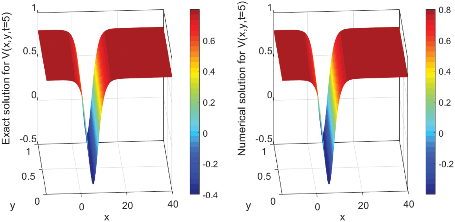
Figure 1: Surface plot of V (x, y, t) presenting the analytical (left) and the numerical (right) solutions’ evolution in time t = 5 using N = 3000 with Δx = 0.02 and M = 100 with Δy = 0.01. The parameter values are A2 = 1.2, β = −0.5, α = 2.70, and γ = −2.20

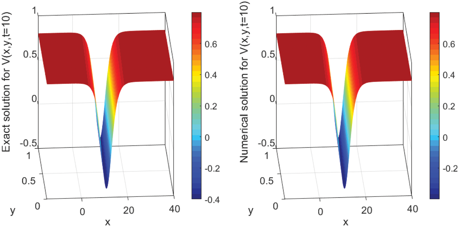
Figure 2: Surface plot of V (x, y, t) presenting the analytical (left) and the numerical (right) solutions’ evolution in time t = 10 using N = 3000 with Δx = 0.02 and M = 100 with Δy = 0.01. The parameter values are A2 = 1.2, β = −0.5, α = 2.70, and γ = −2.20

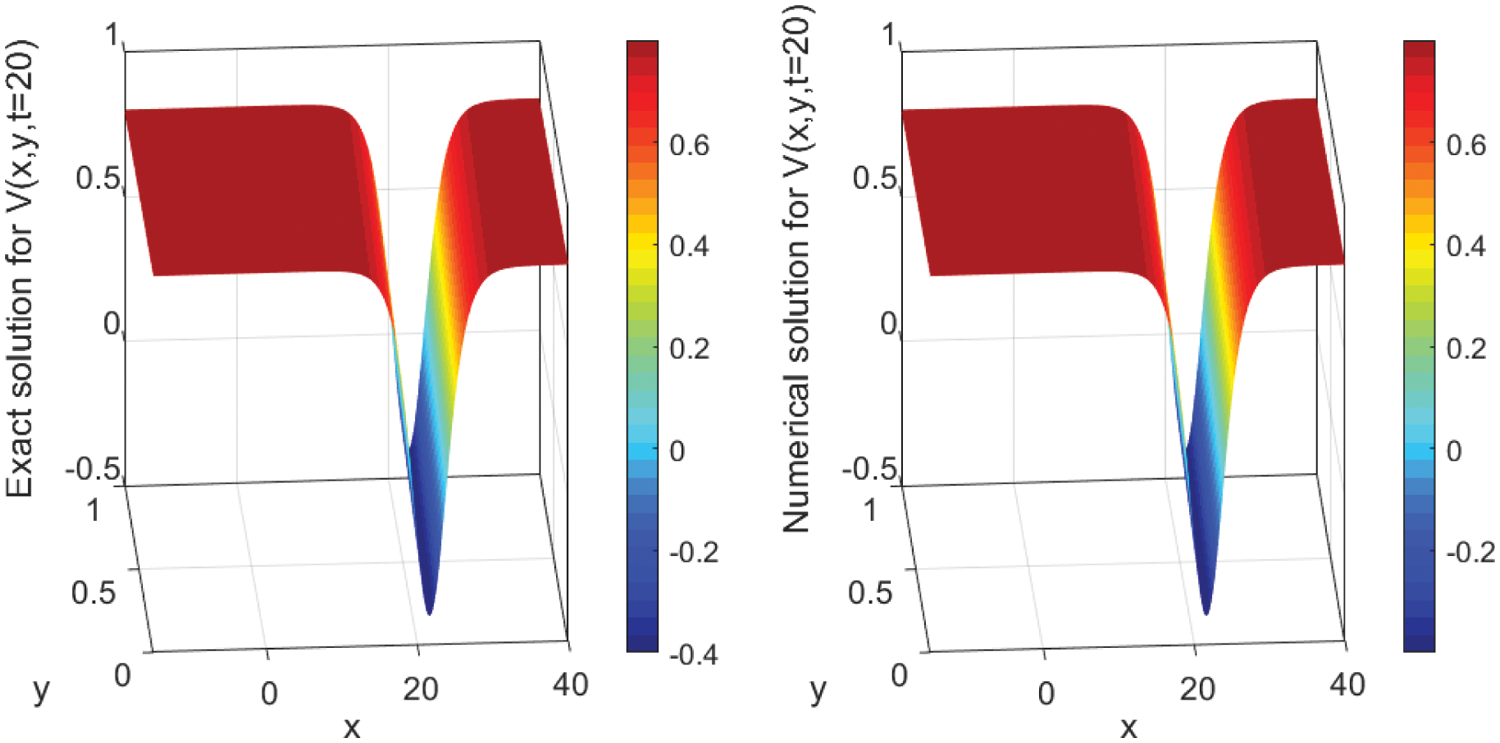
Figure 3: Surface plot of V (x, y, t) presenting the analytical (left) and the numerical (right) solutions’ evolution in time t = 20 using N = 3000 with Δx = 0.02 and M = 100 with Δy = 0.01. The parameter values are A2 = 1.2, β = −0.5, α = 2.70, and γ = −2.20

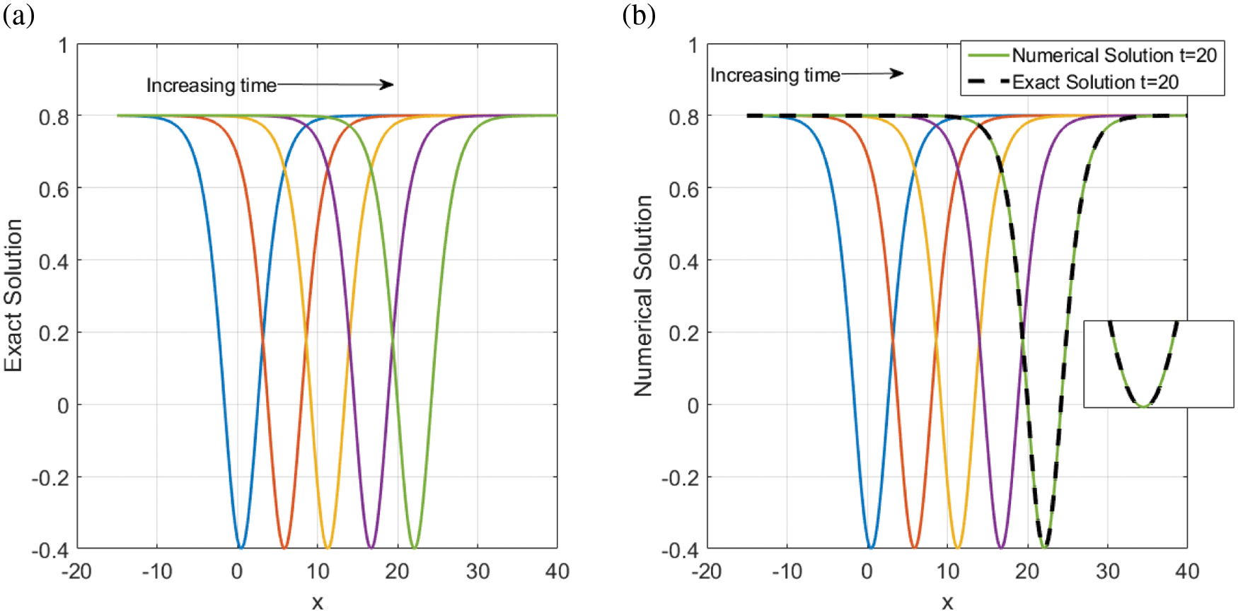
Figure 4: Time evolution of V (x, y, t) to the traveling wave structures (a) the analytical and (b) the numerical solutions with parameter values A2 = 1.2, β = −0.5, α = 2.70, and γ = −2.20. (b) also illustrates the performance of the used approaches

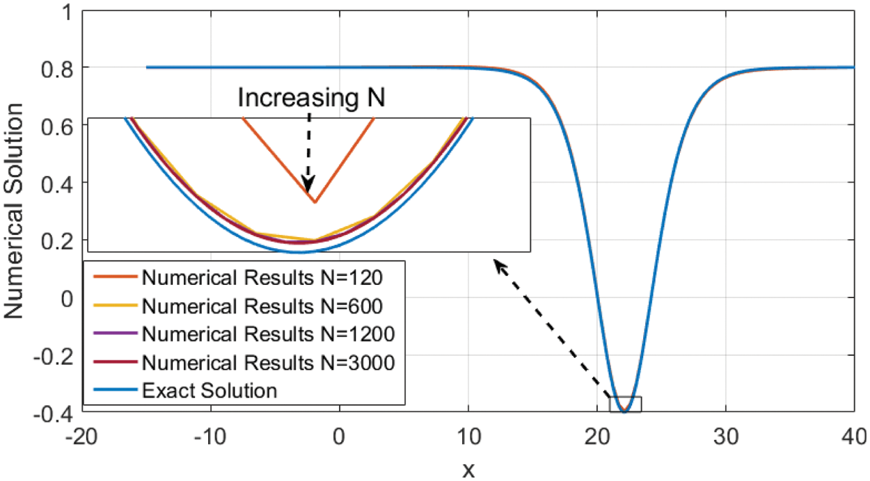
Figure 5: Presents a comparison of the numerical results of Eq. (31) at t = 20 for increasing N of the spatial variable x. The solid blue line shows the exact solution Eq. (12). The parameter values are A2 = 1.2, β = −0.5, α = 2.70, and γ = −2.20. The insets present zoomed-in wave characteristics

Table 1 illustrates L2 errors and the CPU times taken to reach t=20. The error decreases for large N but the method takes more time to give a small error. We begin with N=120, Δx=0.50 and Δy=0.01. The L2 error stands at 5.37×10−4 during 0.74 min. When we use N=3000 with Δx=0.02 and Δy=0.01, the L2 error dramatically decays and stands at 1.073×10−6 during 20.63 min. Fig. 6 shows the decay in the L2 error as N increases.

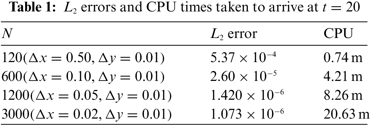
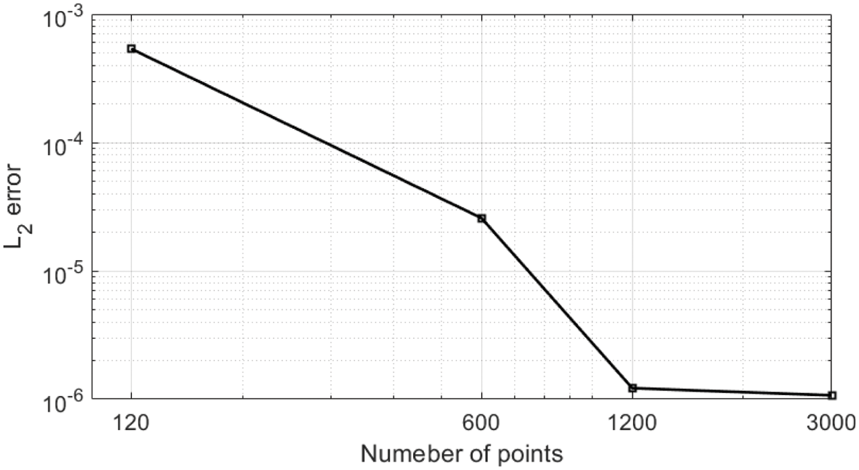
Figure 6: Illustrating L2 errors presenting in Table 1

10  Conclusion

We have favorably implemented an accurate finite difference method on a uniform mesh and the generalized exponential rational function method for the two-dimensional Riemann problems. The main advantage of the results is to show the traveling wave structures and prove their accuracy using numerical methods. By comparing the exact solutions using the generalized exponential rational function method with those from the numerical scheme, it was said that the numerical results are almost identical to the analytical results. It is well known that the numerical scheme is stable and allows a meaningful reduction in memory requirements. Using a fine mesh in both spatial variables x and y permits us to resolve the wave-like structures. We can conclude that the used methods can be efficiently applied to more nonlinear evolution models to construct their exact and numerical solutions.

Funding Statement: The author received no specific funding for this study.

Conflicts of Interest: The author declares that they have no conflicts of interest to report regarding the present study.

References

1. Cattani, C., Sulaiman, T. A., Baskonus, H. M., Bulut, H. (2018). Solitons in an in homogeneous Murnaghan’s rods. The European Physical Journal Plus, 133(6), 228. DOI 10.1140/epjp/i2018-12085-y. [Google Scholar] [CrossRef]
2. Jawad, A. J., Petkovic, M. D., Biswas, A. (2010). Modified simple equation method for nonlinear evolution equations. Applied Mathematics and Computation, 217(2), 869–877. DOI 10.1016/j.amc.2010.06.030. [Google Scholar] [CrossRef]
3. Malflieta, W., Hereman, W. (1996). The tanh method: Exact solutions of nonlinear evolution and wave equations. Physica Scripta, 54(6), 563–568. DOI 10.1088/0031-8949/54/6/003. [Google Scholar] [CrossRef]
4. Alharbi, A. R., Almatrafi, M. B., Lotfy, K. (2020). Constructions of solitary travelling wave solutions for Ito integro-differential equation arising in plasma physics. Results in Physics, 19, 103533. DOI 10.1016/j.rinp.2020.103533. [Google Scholar] [CrossRef]
5. Gurefe, Y., Misirli, E., Pandir, Y., Sonmezoglu, A., Ekici, M. (2015). New exact solutions of the davey-stewartson equation with power-law nonlinearity. Bulletin of the Malaysian Mathematical Sciences Society, 38(3), 1223–1234. DOI 10.1007/s40840-014-0075-z. [Google Scholar] [CrossRef]
6. Abdelrahman, M. A. E., Almatrafi, M. B., Alharbi, A. (2020). Fundamental solutions for the coupled KdV system and its stability. Symmetry, 12(3), 429. DOI 10.3390/sym12030429. [Google Scholar] [CrossRef]
7. Alharbi, A. R., Almatrafi, M. B. (2020). Analytical and numerical solutions for the variant Boussinseq equations. Journal of Taibah University for Science, 14(1), 454–462. DOI 10.1080/16583655.2020.1746575. [Google Scholar] [CrossRef]
8. Ghanbari, B., Yusuf, A., Inc, M., Baleanu, D. (2019). The new exact solitary wave solutions and stability analysis for the (2 + 1)-dimensional Zakharov–Kuznetsov equation. Advances in Difference Equations, 49(1), 1–15. DOI 10.1186/s13662-019-1964-0. [Google Scholar] [CrossRef]
9. Almatrafi, M. B., Alharbi, A. R., Tunç, C. (2020). Constructions of the soliton solutions to the good Boussinesq equation. Advances in Difference Equations, 2020(1), 629. DOI 10.1186/s13662-020-03089-8. [Google Scholar] [CrossRef]
10. Alharbi, A. R., Almatrafi, M. B., Seadawy, A. R. (2020). Construction of the numerical and analytical wave solutions of the Joseph-Egri dynamical equation for the long waves in nonlinear dispersive systems. International Journal of Modern Physics B, 34(30), 2050289. DOI 10.1142/S0217979220502896. [Google Scholar] [CrossRef]
11. Alharbi, A. R., Almatrafi, M. B., Lotfy, K. (2020). Constructions of solitary traveling wave solutions for ito integro-differential equation arising in plasma physics. Results in Physics, 19, 103533. DOI 10.1016/j.rinp.2020.103533. [Google Scholar] [CrossRef]
12. Alharbi, A., Almatrafi, M. B. (2020). Exact and numerical solitary wave structures to the variant Boussinesq system. Symmetry, 12(9), 1473. DOI 10.3390/sym12091473. [Google Scholar] [CrossRef]
13. Alharbi, A. R., Almatrafi, M. B. (2020). New exact and numerical solutions with their stability for ito integro-differential equation via Riccati–Bernoulli sub-ODE method. Journal of Taibah University for Science, 14(1), 1447–1456. DOI 10.1080/16583655.2020.1827853. [Google Scholar] [CrossRef]
14. Alharbi, A. R., Almatrafi, M. B. (2020). Numerical investigation of the dispersive long wave equation using an adaptive moving mesh method and its stability. Results in Physics, 16, 102870. DOI 10.1016/j.rinp.2019.102870. [Google Scholar] [CrossRef]
15. Alharbi, A. R., Almatrafi, M. B. (2020). Riccati-Bernoulli sub-ODE approach on the partial differential equations and applications. International Journal of Mathematics and Computer Science, 15(1), 367–388. [Google Scholar]
16. Jawad, A. J. M., Johnson, S., Yildirim, A. et al. (2013). Soliton solutions to coupled nonlinear wave equations in (2 + 1)-dimensions. Indian Journal of Physics, 87(3), 281–287. DOI 10.1007/s12648-012-0218-8. [Google Scholar] [CrossRef]
17. Alharbi, A., Almatrafi, M. B. (2022). Exact solitary wave and numericalsolutions for geophysical KdV equation. Journal of King Saud University-Science, 34(6), 102087. DOI 10.1016/j.jksus.2022.102087. [Google Scholar] [CrossRef]
18. Shao, Z. (2010). Global structure stability of Riemann solutions for linearly degenerate hyperbolic conservation laws under small BV perturbations of the initial data. Nonlinear Analysis: Real World Applications, 11(5), 3791–3808. DOI 10.1016/j.nonrwa.2010.02.009. [Google Scholar] [CrossRef]
19. Shao, Z. (2018). The Riemann problem for the relativistic full euler system with generalized chaplygin proper energy density-pressure relation. Zeitschrift für Angewandte Mathematik und Physik, 69(2), 1420–9039. DOI 10.1007/s00033-018-0937-6. [Google Scholar] [CrossRef]
20. Chen, Y., Li, B., Zhang, H. Q. (2003). Symbolic computation and construction of soliton-like solutions to the (2 + 1)-dimensional breaking soliton equation. Communications in Theoretical Physics, 40(6), 137. DOI 10.1088/0253-6102/40/2/137. [Google Scholar] [CrossRef]
21. Peng, Y. (2003). New exact solutions for (2 + 1)-dimensional breaking soliton equation. Communications in Theoretical Physics, 43(2), 205. DOI 10.1088/0253-6102/43/2/004. [Google Scholar] [CrossRef]
22. Abdelrahman, M. A. E., Alharbi, A. (2021). Analytical and numerical investigations of the modified camassa-holm equation. Pramana Journal, 95(3), 117. DOI 10.1007/s12043-021-02153-6. [Google Scholar] [CrossRef]
23. Brown, P. N., Hindmarsh, A. C., Petzold, L. E. (1994). Using Krylov methods in the solution of large-scale differential-algebraic systems. SIAM Journal on Scientific Computing, 15(6), 1467–1488. DOI 10.1137/0915088. [Google Scholar] [CrossRef]
24. Chandrasekhar, S. (1981). Hydrodynamic and hydromagnetic stability. New York, USA: Dover Publications Inc. [Google Scholar]
25. Brown, P. N., Hindmarsh, A. C., Petzold, L. R. (1994). Using Krylov methodsin the solution of large-scale differential-algebraic systems. Society for Industrial and Applied Mathematics Journal on Scientific Computing, 15(6), 1467–1488. DOI 10.1137/0915088. [Google Scholar] [CrossRef]
Cite This Article
Copyright © 2023 The Author(s). Published by Tech Science Press.
This work is licensed under a Creative Commons Attribution 4.0 International License , which permits unrestricted use, distribution, and reproduction in any medium, provided the original work is properly cited.
Downloads
Citation Tools