
 Submit a Paper
 Propose a Special lssue
 Open Access
ARTICLE
Structural Damage Identification Using Ensemble Deep Convolutional Neural Network Models
1
Department of Civil and Environmental Engineering, Amirkabir University of Technology, Tehran, Iran
2
Department of Urban Planning, Engineering Networks and Systems, Institute of Architecture and Construction, South Ural State
University, Chelyabinsk, Russian
3
Department of Computational Mechanics Laboratory, School of Pedagogical and Technological Education, Athens, Greece
* Corresponding Author: Danial Jahed Armaghani. Email:
(This article belongs to the Special Issue: Soft Computing Techniques in Materials Science and Engineering)
Computer Modeling in Engineering & Sciences 2023, 134(2), 835-855. https://doi.org/10.32604/cmes.2022.020840
Received 15 December 2021; Accepted 29 April 2022; Issue published 31 August 2022
 View Full Text
 Download PDF
Abstract
The existing strategy for evaluating the damage condition of structures mostly focuses on feedback supplied by traditional visual methods, which may result in an unreliable damage characterization due to inspector subjectivity or insufficient level of expertise. As a result, a robust, reliable, and repeatable method of damage identification is required. Ensemble learning algorithms for identifying structural damage are evaluated in this article, which use deep convolutional neural networks, including simple averaging, integrated stacking, separate stacking, and hybrid weighted averaging ensemble and differential evolution (WAE-DE) ensemble models. Damage identification is carried out on three types of damage. The proposed algorithms are used to analyze the damage of 4585 structural images. The effectiveness of the ensemble learning techniques is evaluated using the confusion matrix. For the testing dataset, the confusion matrix achieved an accuracy of 94 percent and a minimum recall of 92 percent for the best model (WAE-DE) in distinguishing damage types as flexural, shear, combined, or undamaged.Keywords
Nomenclature
| CNN | Convolutional Neural Network |
| SHM | Structural Health Monitoring |
| PEER | Pacific Earthquake Engineering Research |
| PHI | Center Hub ImageNet |
| F | Flexural Damage |
| S | Shear Damage |
| FS | Combined Damage |
| UN | Undamaged Condition |
| SAE | Simple Averaging Ensemble |
| WEA | Weighted Averaging Ensemble |
| DE | Differential Evolution |
| SSM | Separate Stacking Ensemble |
| SVM | Support Vector Machine |
| ISE | Integrated Stacking Ensemble |
| CM | Confusion Matrix |
Artificial intelligence (AI) methods have had a significant impact on a variety of disciplines, ranging from engineering applications, health sciences, intelligent games, to material discovery [1]. Machine learning (ML) methodologies and computing power advancements facilitate not only the handling of big data within reasonable time restrictions, but also the automatic discovery of underlying patterns of the data without requiring human subjective judgments [2,3]. The decision-making process may become more reliable and efficient using ML models [4]. The application of ML algorithms in civil engineering involves a wide range of disciplines [5–7], including structural health monitoring [8,9], geotechnical engineering [7], and structural and earthquake engineering [10–12]. Das et al. [13] adopted a deep convolutional neural network (CNN) to determine crack patterns in strain hardening cementitious composites. The proposed model can predict crack metrics such as average crack width and crack density based on the crack pattern. Abdelkader [14] proposed a hybrid pre-trained deep learning algorithm for the crack identification in various infrastructures using visual geometry group networks, K-nearest neighbors, and differential evolution algorithms. Reis et al. [15] proposed methodologies for classifying images of cracks in historical buildings using a deep learning architecture. Wan et al. [16] assessed an encoder-decoder network-based architecture for identifying pavement cracks with intricate textures under various illumination situations. Bigdeli et al. [17] used a new architecture based on CNNs for densifying crack bifurcation in concrete structures. Mohammed et al. [18] utilized various established open-source CNNs to evaluate their detection accuracy in concrete crack classification. Ye et al. [19] used CNNs, a bridge crack library, to develop a model for structural crack detection of multiple structural materials such as masonry, concrete, and steel. Flah [20] presented an automated inspection framework based on image processing and deep learning techniques to identify defects in otherwise difficult to access regions of concrete structures. Wang et al. [21] developed a structural damage identification framework based on time-frequency graphs and the marginal spectrum of the signals using CNNs and particle swarm optimization algorithm. Meng et al. [22] introduced a modified CNN for long-term structural monitoring using both forward convolution and reverse convolution. Quqa et al. [23] utilized image processing techniques and CNNs for crack identification in steel bridges using an image dataset of the welded joints of steel bridges. Sharma et al. [24] suggested a one-dimensional CNN for detecting damaged joints in semi-rigid frames. A novel procedure is suggested by Sony et al. [25] based on a windowed one-dimensional CNN for multiclass damage detection using vibration responses on a full-scale bridge. Alazzawi et al. [26] proposed a deep residual network to extract characteristics from raw response signals recorded from steel beams under various damage situations. Yang et al. [27] presented a CNN-U-Net architecture model combined with a nonlinear regression model for identifying the crack skeleton. The different research studies cited above classified structural damage in structural members using typical DL-based models, which involve classifying the damage using a set of pictures from the desired damage type. However, these ML algorithms still have flaws, such as being inaccurate or weak, having limited generalization capacity, and running at a low speed [28,29].
After a seismic event, a quick and accurate assessment of the damage level of structures is crucial for emergency action and recovery design. Visual identification is commonly used in current quick damage evaluation methodologies. However, visually detecting and classifying existing reinforced concrete structural damage can be laborious. To this end structural health monitoring (SHM) and fast and easy damage assessment following natural disasters has gained significant research interest. In civil engineering design, using DL in vision-based SHM is a relatively recent research direction and to this end some significant challenges remain to be addressed as researchers try to apply these concepts to structural engineering concerns. For example, there is a lack of a standardized automated identification principle or framework based on existing knowledge with acceptable accuracy for structural damage identification. To this end this research evaluates the feasibility of using ensemble learners, including simple averaging, weighted averaging, integrated stacking, and separate stacking ensemble models, to assess the earthquake-induced damage of reinforced concrete structural members. Ensemble models are developed for structural damage identification using deep convolutional neural network models. Damage type corresponds to a complicated vision pattern that is divided into three categories: flexural, shear, and combined damage. The paper is structured as follows: The data are presented in detail in Section 2. Section 3 describes the CNN and ensemble learning techniques models. Section 4 explains the results and discussion , and Section 5 presents the main conclusions.
In general, reinforced concrete member failures can be divided into three main categories: flexural, shear and flexural-shear. Mechanical characteristics of the reinforced concrete members are directly affected by damage type. In this research, a damage-type dataset was obtained from the Pacific Earthquake Engineering Research (PEER) Center Hub ImageNet (PHI) website [30,31]. A total of 4585 images were available in this dataset, comprising the three damage types defined as flexural (F) damage, shear (S) damage, combined (FS) damage, and also the undamaged (UN) condition. Mechanical characteristics and seismic design are directly affected by damage type. Label definitions corresponding to failure type are presented by Moehle [32] and based on engineering judgment as follows: (1) Flexural-type damage is defined as most cracks occurring in the horizontal or vertical directions, or at the end of an element having vertical or horizontal planes, (2) Shear-type damage is defined when the majority of cracks run diagonally or create a “X” or “V” pattern, and (3) It is classified as combined-type damage if the crack distribution is uneven or accompanied by severe spalling. Images have dimensions as high as 224 × 224 × 3, where 224 × 224 is the resolution (pixels) and the last dimension (3) is the number of the color channels. Table 1 shows the number of images for each damage type. Fig. 1 shows examples of images in the database. In this study, the ML models are developed on the basis of a random split of the data into a training set (70%), a validation set (15%), and a testing set (15%).
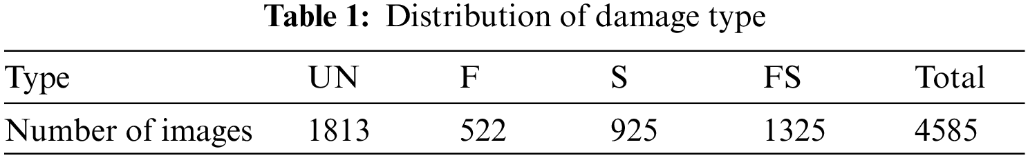
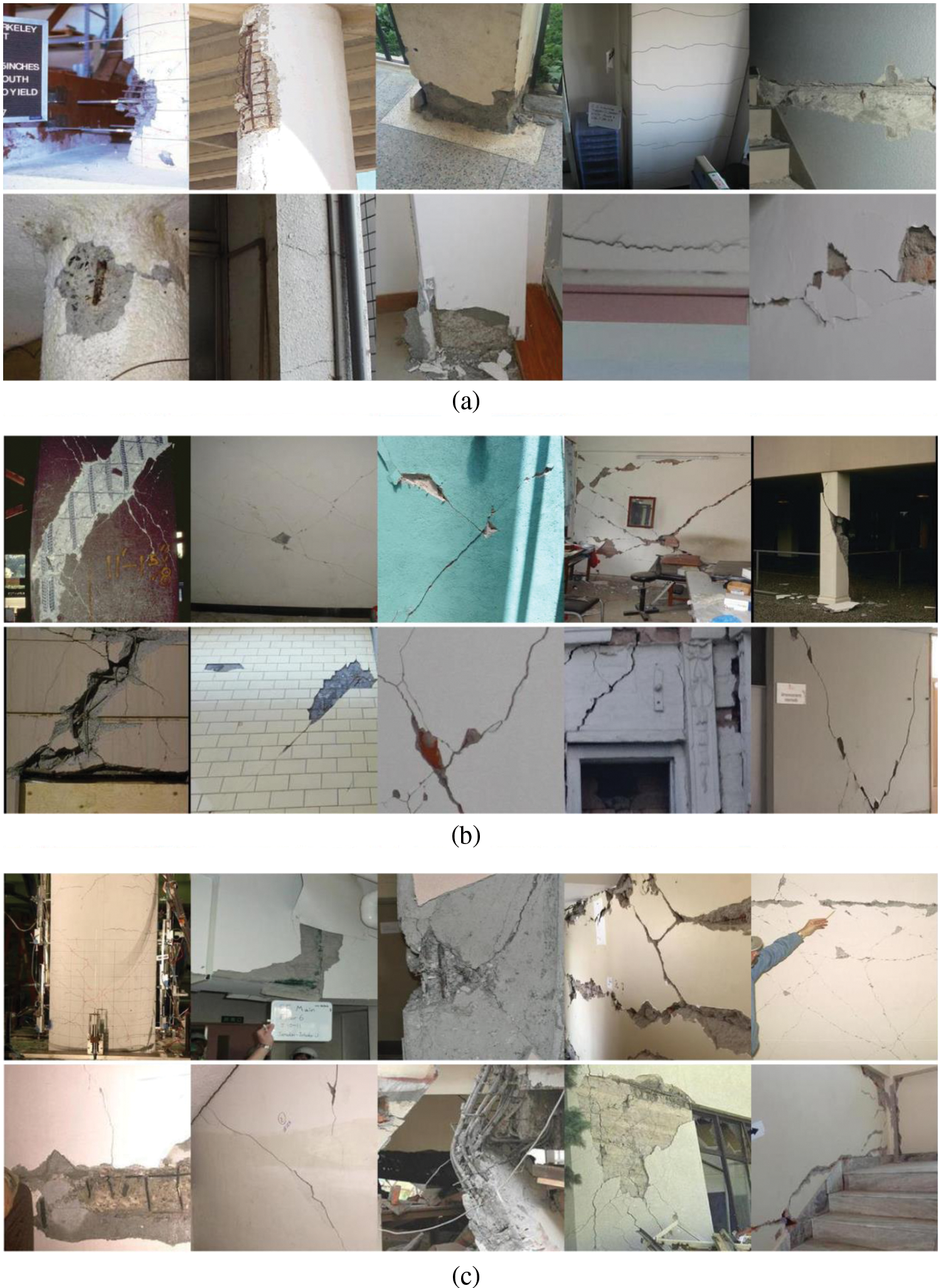
Figure 1: Sample images of the database; (a) F damage, (b) S damage, and (c) FS damaged [30,31]
In this research, ensemble neural network models and super learner ensemble are used to characterize different damage types. The ensemble neural network models use deep neural networks such as base sub-models, but super learner ensemble use bagging and boosting algorithms as base sub-models. The ensemble neural network models developed in this research are simple averaging, weighted averaging, integrated stacking, and separate stacking ensemble models.
A deep convolutional neural network (DCNN) architecture comprises several layers: an input layer, a convolutional layer, a pooling/dropout layer, fully connected layer, and ultimately output layer. As an example, a configuration of a binary classification is illustrated in Fig. 2. A picture is received by the first layer (Input layer). The input data is then processed by the architecture, which reduces its size. Finally, based on the type of categorization, the Softmax layer predicts the final output. For the binary classification, the prediction is based on whether or not the image belongs to a specific group, those classification tasks that have two class labels. For a multi-purpose, classification tasks have more than two class labels.
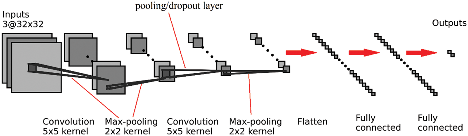
Figure 2: Architecture of the DCNN classifier
In this research, five convolutional network models (CNN) are utilized as the base learners (sub-models). The number of base learners is determined using a trial and error method. These models are created by modifying deep learning models, including a MobileNetV2 [33] and NASNetMobile [34], to capture global context and local deep learning characteristics. This research employs the transfer learning technique (TLT). TLT is a strategy in which a model that was trained to address one problem is reapplied to solve a new problem that is related to the original [35]. Typically, the early layers of an image recognition model will learn to identify generic traits, while the later layers will be able to recognize more specific traits [35,36]. The last layer of an image recognition model will have N Softmax neurons (assuming we are classifying N classes); therefore, it should be modified appropriately and in some cases additional layers may be required. The important step, is fine-tuning, which involves unfreezing the entire model obtained above and re-training it using the new data with a very low learning rate.
MobileNetV2 and NASNetMobil have a total of 88 and 769 layers, respectively [33,34]. CNNs architectures of the sub-models are shown in Fig. 3. The additional layers are highlighted in green. The simple averaging, weighted averaging, integrated stacking, and separate stacking ensemble models are created using these sub-models.
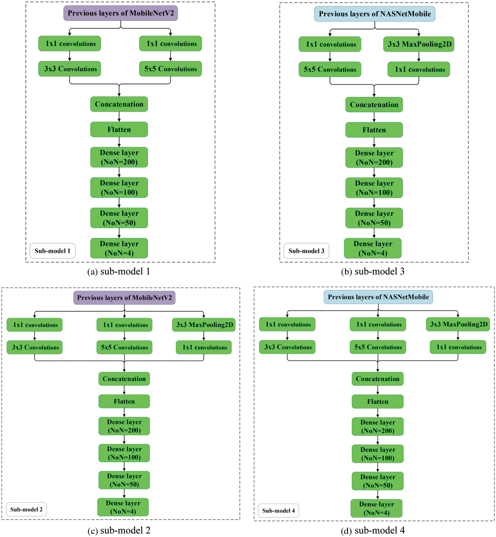
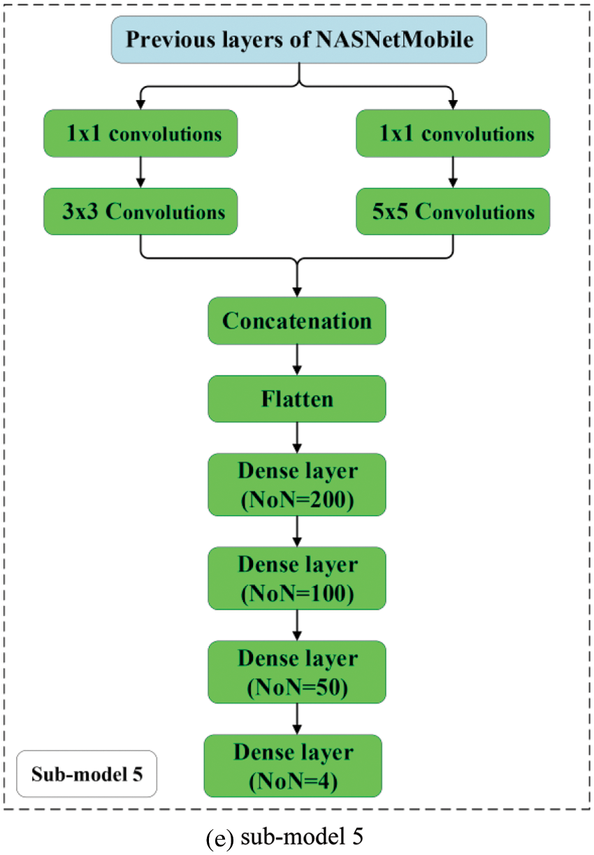
Figure 3: Architectures of the sub-models
For numerical purposes, averaging is the most common and basic combination approach. Simple averaging ensemble (SAE) is one of the most widely used approaches [37], and it is often the first choice in many real-world applications due to its simplicity and efficacy. By directly averaging the outputs of the sub-models, simple averaging yields the total output. Here, five CNN base learners (Section 3.2) are considered for developing the SAE. A diagram of the SAE process is illustrated in Fig. 4.
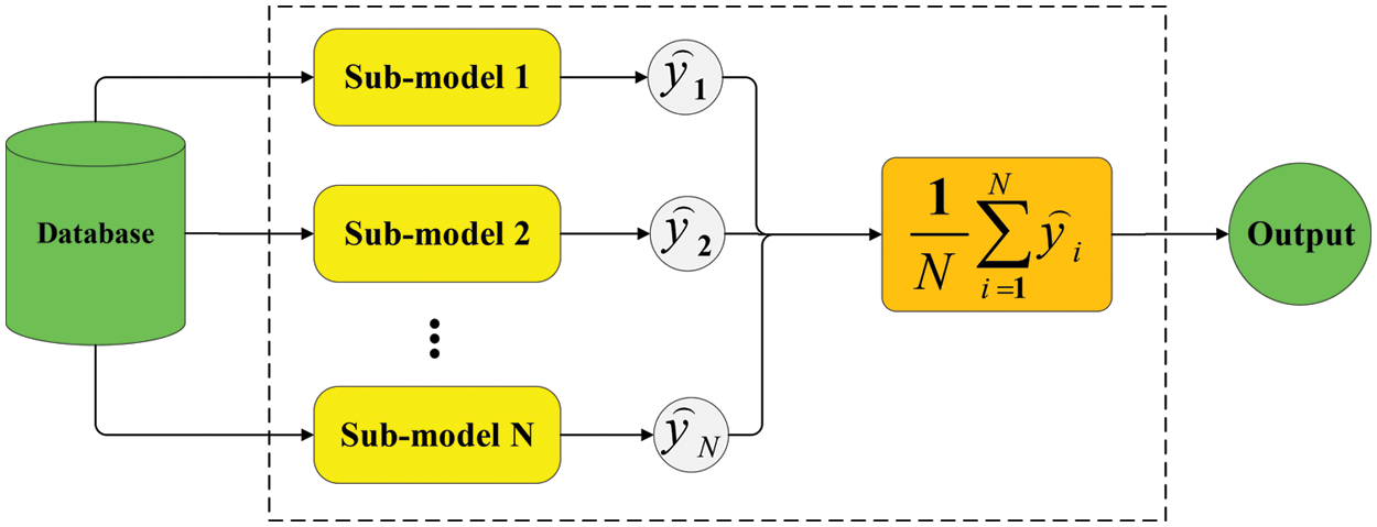
Figure 4: Simple averaging method
3.4 Weighted Averaging Ensemble
The simple averaging technique assigns the same weight to all sub-models. The weighted averaging ensemble (WEA), generates a combined output by averaging each sub-model output by varying the assigned weights. Determining the weights may be computationally challenging, and optimization algorithms are usually employed at this stage [38]. In this research, differential evolution (DE) is employed to determine the weights in the WEA [39,40]. DE is a vector-based technique that, due to its usage of crossover and mutation, is similar to pattern searching and genetic algorithms [39,40]. DE is a self-organizing search method that does not rely on derivative information. As a result, it is a population-based, derivative-free approach. DE uses the population’s directional data. Each member of the present generation is allowed to reproduce by mating with other randomly chosen members of the population. For each individual, three other separate individuals are randomly selected. As a result, to breed an offspring, a parent pool of four individuals is generated. After initialization, DE uses mutation to build a mutated vector relating to each population member, and then uses arithmetic recombination to construct a target vector in the present generation. Differentiating one DE scheme from another is the procedure of creating the modified vector. In DE, mutation occurs before crossover, whereas in genetic algorithms, mutation occurs after crossover. Furthermore, mutation is used less frequently in genetic algorithm, whereas it is used on a regular basis in DE to develop each offspring. Fig. 5 shows the conceptual schematic of the WAE-DE hybrid algorithm.
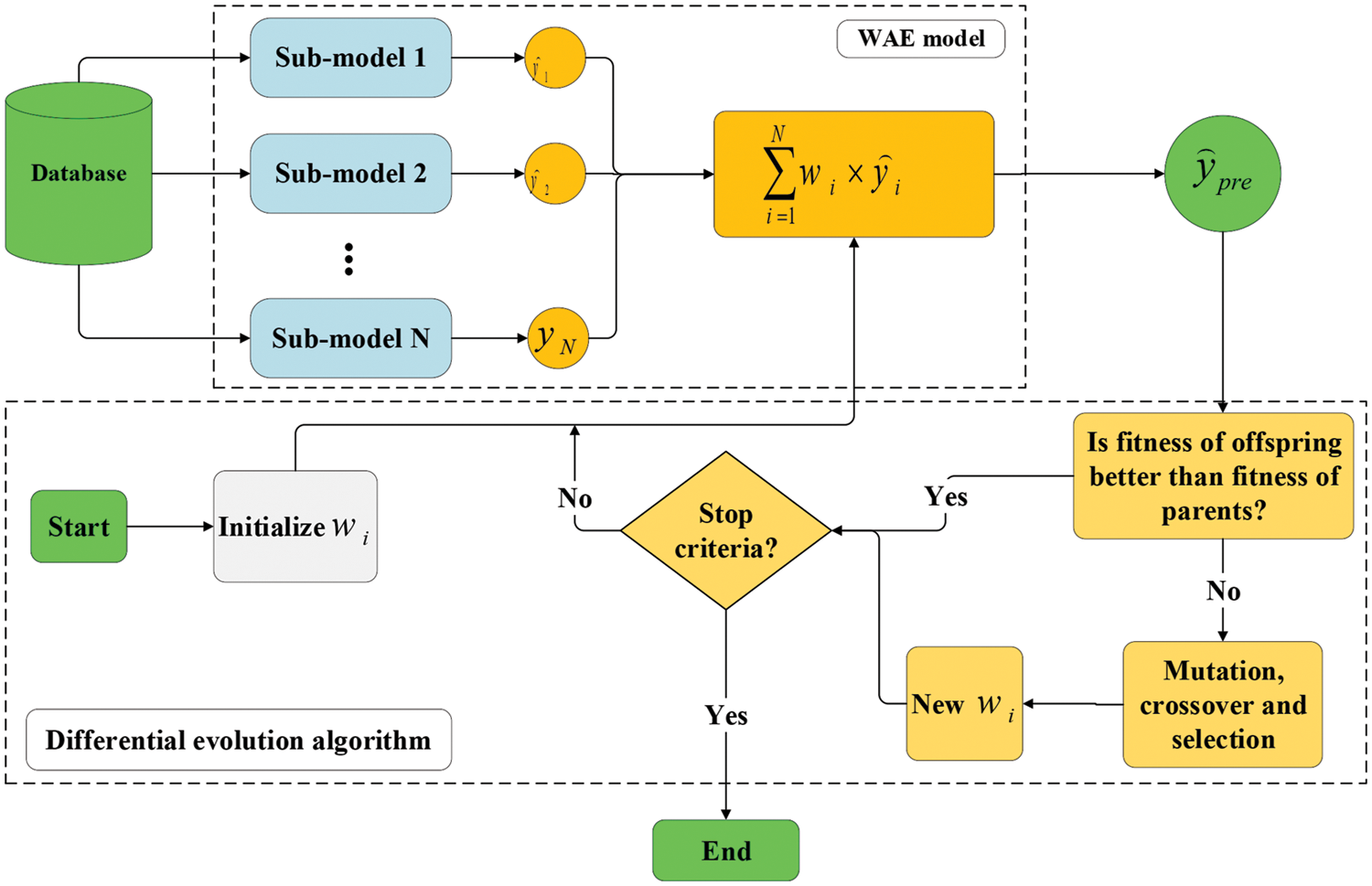
Figure 5: Conceptual schematic of the WAE-DE algorithm
Stacking is another ensemble learning approach that employs a meta-model to integrate a large number of the sub-models (usually heterogeneous learners) to provide a more accurate final prediction than a single model (Fig. 6) [41]. The predictions returned by the sub-models are then aggregated by training a meta-model based on the outputs of individual sub-models. The term “integrated stacking” is used when the meta-model is a neural network; otherwise, “separate stacking” is used.
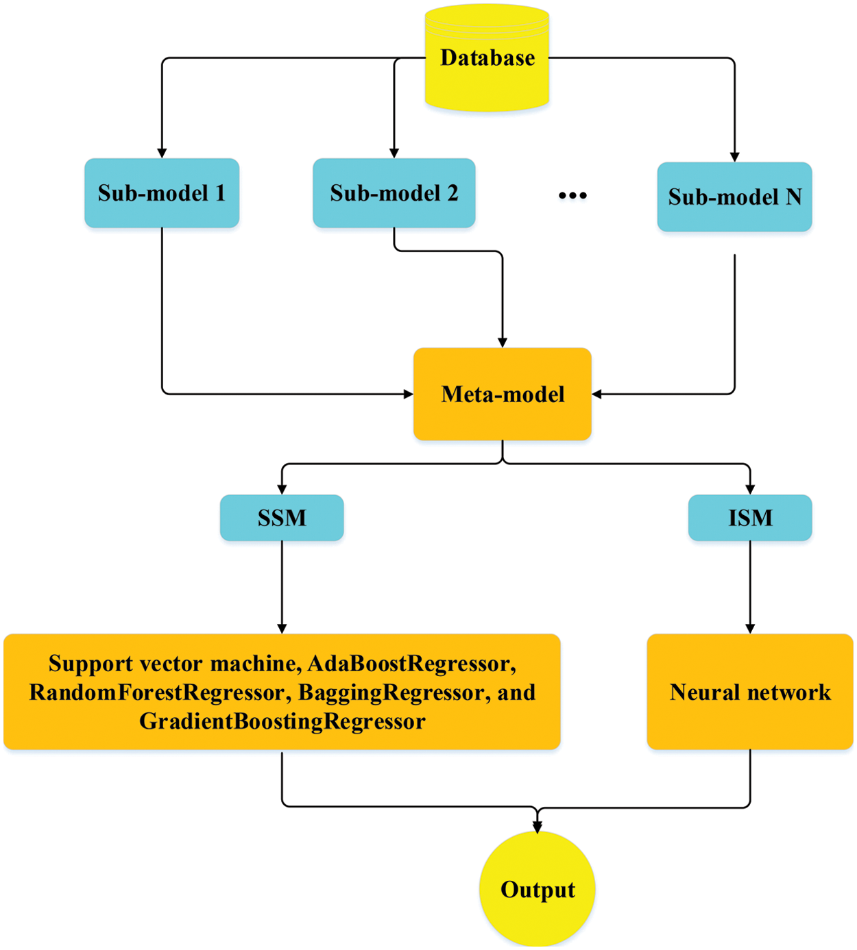
Figure 6: Stacking ensemble algorithms workflow
3.5.1 Separate Stacking Ensemble (SSM)
In this research, SSMs are generated with sub-models (Section 3.2) and five different meta-models, including support vector machine, Adaptive Boosting (AdaBoost), RandomForest, Bagging, and Gradient Boosting (GraBoost), default parameters are used for meta-models. Support vector machine (SVM) is firstly developed for classification of different classes. The strategy is that the sample points (input) are transformed into a higher-dimensional feature space using a linear/nonlinear transformation. Then a hyperplane is used to describe the classification. SVM regression is generally regarded as a nonparametric method because it relies on kernel functions. A kernel is used to identify a hyperplane in a higher-dimensional space while reducing the computing cost. When we use SVM, our major goal in the regression problem is to choose a decision boundary that is a certain distance from the initial hyperplane and contains data points that are closest to the hyperplane. AdaBoost is a collection of numerous decision trees, each of which is a poor learner and performs just marginally better than arbitrary guessing [42]. The AdaBoost method transmits the gradient of previous trees to subsequent trees in order to minimize the error of the prior tree. As a result, the subsequent learning of trees at each step contributes to the development of a strong learner. The ultimate prediction is a weighted average of each tree’s projections. AdaBoost is more resistant to outliers and noisy data due to its strong flexibility. Bagging is a condensed version of bootstrap aggregation. It is an ensemble technique that splits a dataset into m samples, and samples sets do not need to be disjointed. After that, each of the m samples is trained separately into m different machine learning models. The outputs of all the different models are then integrated into a single output via for example voting or averaging. Random Forest (RF) is a Bagging extension in which randomized feature selection is incorporated [43]. At each step of split selecting in the construction of a decision tree, RF first takes a subset of features at random, then performs the traditional split selection technique inside the selected feature subset. Graboost is comparable to other methods of boosting [44]. Since it is necessary to incrementally raise or boost weak learners, unlike AdaBoost, which involves adding a new learner after increasing the weight of poorly predicted data, gradient boosting involves training a new model based on residual errors from the preceding prediction.
3.5.2 Integrated Stacking Ensemble (ISE)
When employing deep neural networks as a sub-model, a neural network may be a preferable choice as a meta-model. In the ISE algorithm, a neural network is used as a meta learner. The sub-models can be inserted in a larger network that the meta-model learns how to combine the sub-models’ outputs in the best way possible. In this work, a shallow neural network consisting of only 1 hidden layer with 25 neurons is selected as the meta-model. The number of neurons in hidden layer has been determined using trial and error method. The activation function and optimizer are “Tanh” and “Adm”, respectively.
A confusion matrix (CM) is used to assess the effectiveness and efficiency of each ML model in greater depth. The CM is a table that compares the observed and predicted damage. The metrics utilized to assess the performance of the models are in Eqs. (1)–(3):
A TP is when the model forecasts the positive class properly. A TN, on the other hand, is a result in which the model accurately forecasts the negative class. A FP occurs when the model forecasts the positive class inaccurately. And a FN is an output in which the model forecasts the negative class inaccurately. Recall and Precision are very useful when dealing with unbalanced datasets [45].
In Fig. 7, F, S, FS, and UN stand for flexural damage, shear damage, combined (flexural-shear) damage, and undamaged. The diagonal cells in the CM reflect the classes that the algorithm properly detected, whereas the off-diagonal cells denote the classes that were mistakenly predicted. The accuracy (Eq. (1)) is shown in the lowest cell on the right side of the CM (i.e., fifth row and fifth column, Fig. 7). The precision metric (Eq. (2)) is indicated by the column on the far right of the CM. The recall metric (Eq. (3)) is indicated by the row at the bottom of the CM. Fig. 7 reports the CM of each sub-model for the testing phase. It can be recognized that the worst classification accuracy is represented for the sub-model 1 with a value of 82.7%. The highest accuracy has been recorded for the sub-model 4 with a value of 89.97%. Although the sub-model 4 has the highest accuracy, Recall values of the sub-model 3 for all classes are higher than 84%.
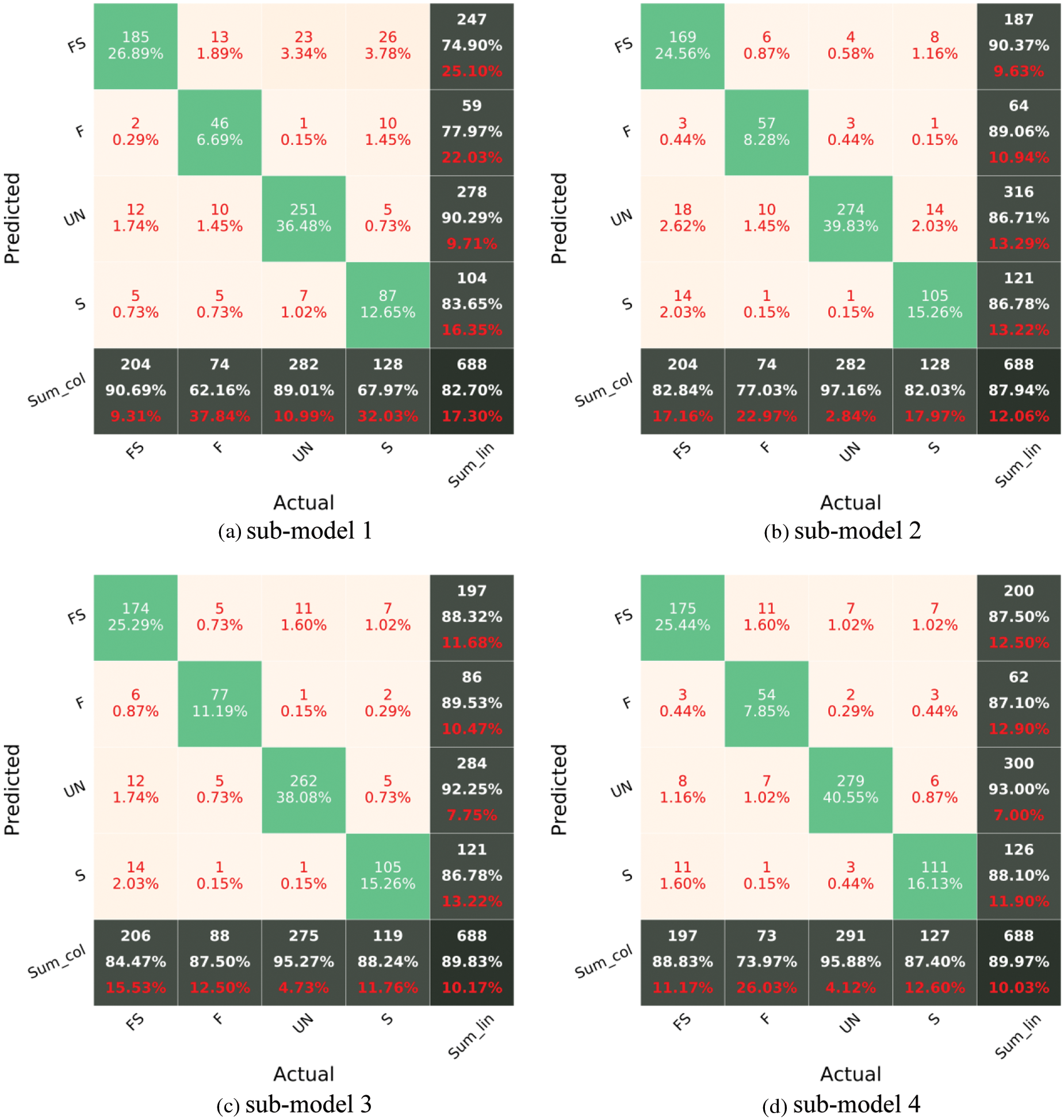
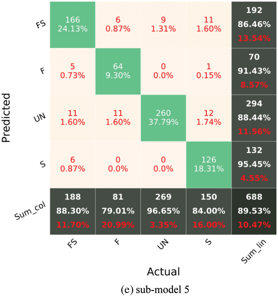
Figure 7: Confusion matrix of sub-models using the testing set
The number of members in the SAE method can affect the outcome. As a result, the impact of the number of base learners (sub-models) on the model performance is investigated, and the ideal number of members is determined. Increasing the size of the ensemble model (adding base learners) is accomplished by first generating a new model using the first two base learners (from Section 3.2), namely sub-model 1 and sub-model 2, and then adding another sub-model to the preceding group for each succeeding model. The accuracy of the model is assessed each time using the test data. Fig. 8 depicts the relationship between the number of members and accuracy. When the model members include the base learner 1 to 4, there is a marked increase from 0.83 to 0.93 in the accuracy of the ensemble models. After that point the accuracy of the SAE reaches a plateau and does not change.
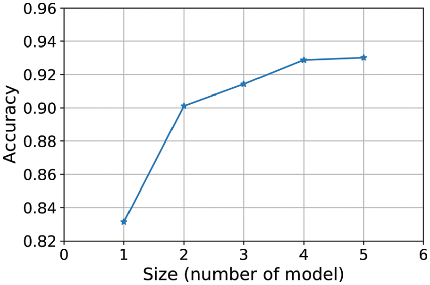
Figure 8: Influence of the number of members
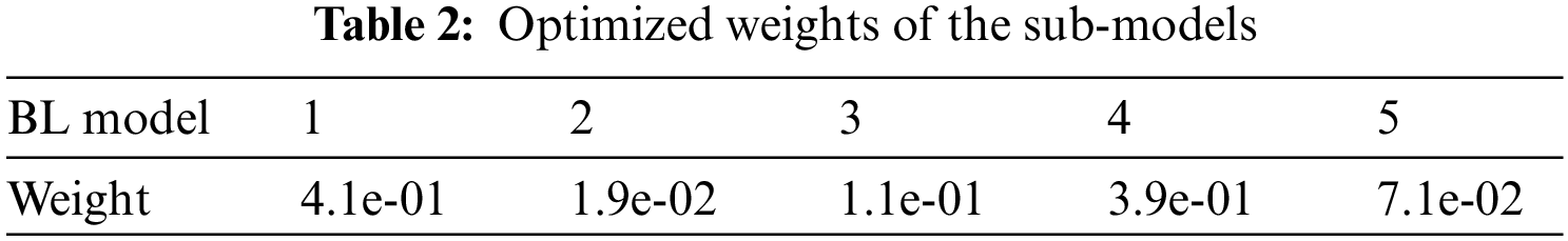
The WAE-DE is the second ensemble learning method. As previously mentioned, the weight of each BL model is computed via the DE algorithm. The weight of each sub-model in WAE-DE is shown in Table 2. Based on Table 2, the sub-models 1 and 4 are given more weight than the others.
The models’ accuracy is assessed using an unknown test set. Fig. 9 shows the CM of various models for the testing phase. For the testing dataset, all models have an accuracy greater than 91%, demonstrating their ability to quickly assess the damage type after an earthquake with reasonable accuracy. The accuracies of the various models are SAE = 91.4%, WAE-DE = 94%, ISE = 93.7% SSM-AdaBoost = 92.7%, SSM-Bagging = 92.4%, SSM-Graboost = 92.7%, SSM-RF = 93.1%, and SSM-SVM = 94%. Among the ensemble models, the WAE-DE and SSM-SVM models fare much better. Meanwhile, the precision and recall of SSM-SVM, ISE, and WAE-DE are greater than 91% for almost all damage classes. While the recognition of FS damage is challenging in other research studies [46,47], the WAE-DE and SSM-SVM model achieved a near 93% recall and 96% precision in identifying the flexure-shear failure type in the testing dataset. Nevertheless, it seems that the prediction of the FS damage is challenging for the other examined models. A modeling averaging ensemble combines the prediction from each model equally and often results in better performance on average than a given single model. Comparison of the performance of the ensemble models (Fig. 9) with the performance of single models (sub-models, Fig. 7) shows the efficiency of the SSM-SVM and WAE-DE models in classifying damage types of RC members. The rate of increase in accuracy in identifying the type of failure is about 4%.
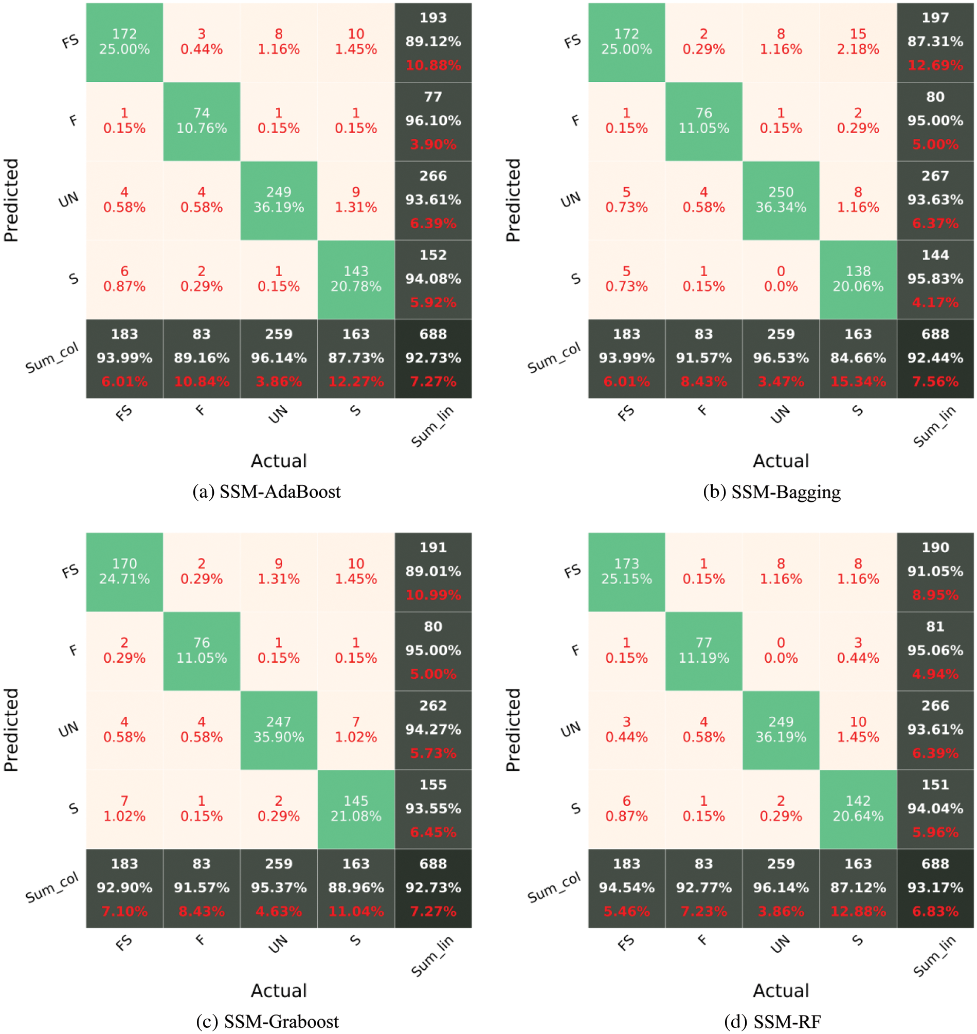
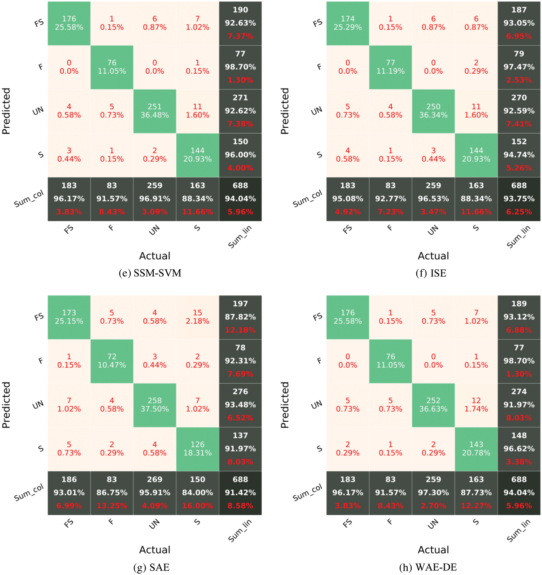
Figure 9: Confusion matrix of various ensemble models for the testing phase
The SAE equalizes the predictions of each model. A weighted average ensemble is a method for allowing different models to contribute to a forecast in proportion to their level of confidence or anticipated performance. WAE-DE (weighted average ensemble) outperforms the SAE [48]. Although model averaging can be upgraded by weighting the influences of each sub-model to the merged prediction by the expected performance of the sub-models, this can be further enhanced by training a completely new model (meta model, such as SVM) to discover how to optimally aggregate the contributions of each sub-model considering nonlinear relationship between inputs and output. Depending on how well the meta model can model the nonlinear relationship between inputs and output, the performance of this type of hybrid model will vary [48].
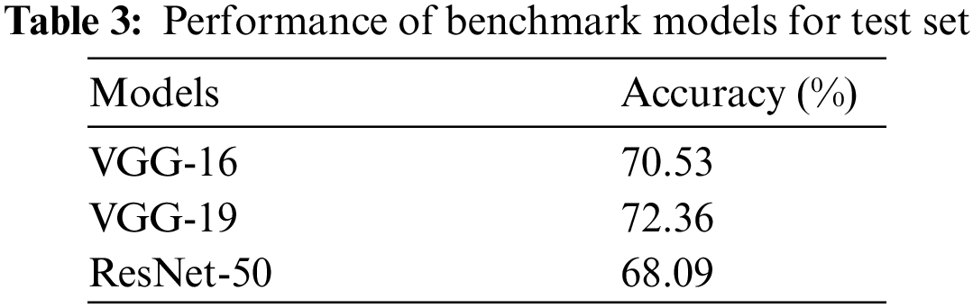
Gao et al. [49] used some well-known deep CNN (benchmark) models, including VGG-16 [50], VGG-19 [50], and ResNet-50 [51] models, for structural damage identification using same database. Table 3 shows the results of the VGG-16, VGG-19, and ResNet-50 models. The best benchmark model (VGG-19) is significantly poorer than the SSM-SVM and WAE-DE models in terms of performance. This emphasizes the significance of choosing the right model for future applications rather than relying on a single model.
The k-fold cross-validation approach may produce a noisy assessment of model performance after just one run [52]. Different data splitting can produce quite various findings. Repeated k-fold cross-validation [52] is a technique for improving assessment of a machine learning model’s performance. In this method, the cross-validation technique is performed several times and return the mean result across all folds from all runs. This mean result is believed to be a more accurate representation of the genuine unknown underlying mean performance of the model on the dataset. As an example, Box-Whisker Plots of performance vs. repeats for k-fold cross-validation for SSM-SVM and SAE model are shown in Fig. 10. The orange line represents the median and the green triangle indicates the arithmetic mean of the distribution. In addition, examining the learning curves of the algorithms during training could be used to discover learning challenges like the overfitting [52]. Overfitting results in a model that is too similar to the inputs, lowering the generalizability of the model. Overfitting leads the validation loss graph to rise at a certain level and does not approach a point of stability. Fig. 11 illustrates an example of overfitting. The models’ curve is depicted in Fig. 11. The validation loss curves approach a point of stability, as shown in Fig. 12.
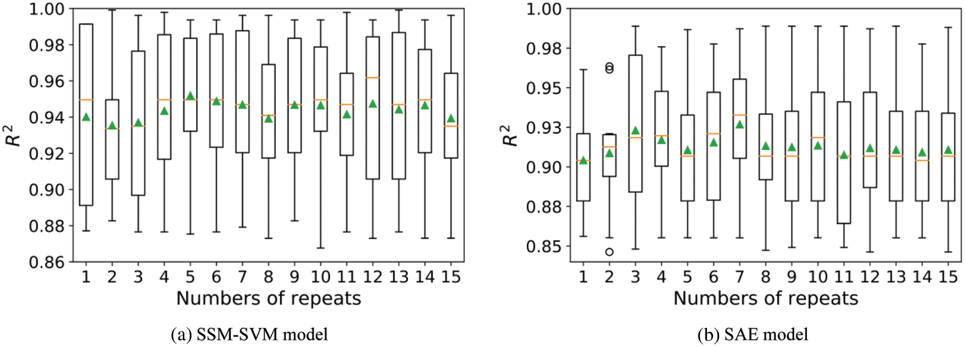
Figure 10: Loss-Epochs curve for a overfitted-model
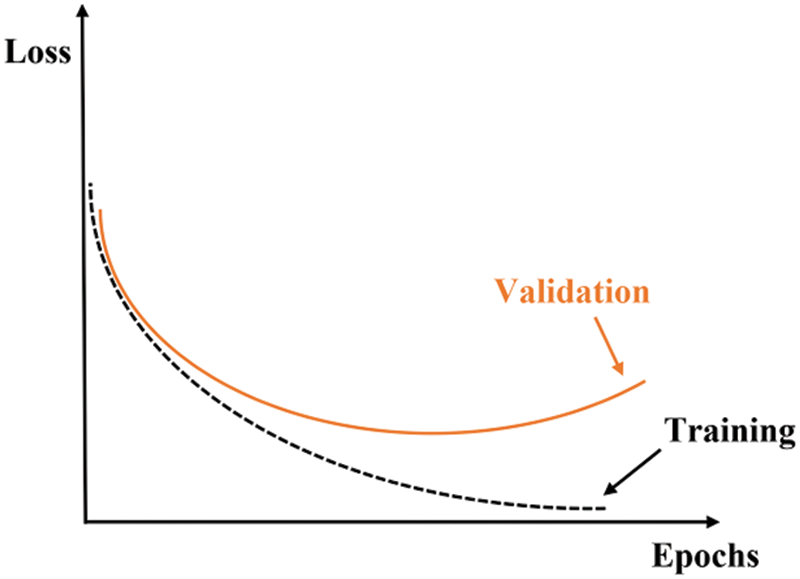
Figure 11: Loss-Epochs curve for a overfitted-model
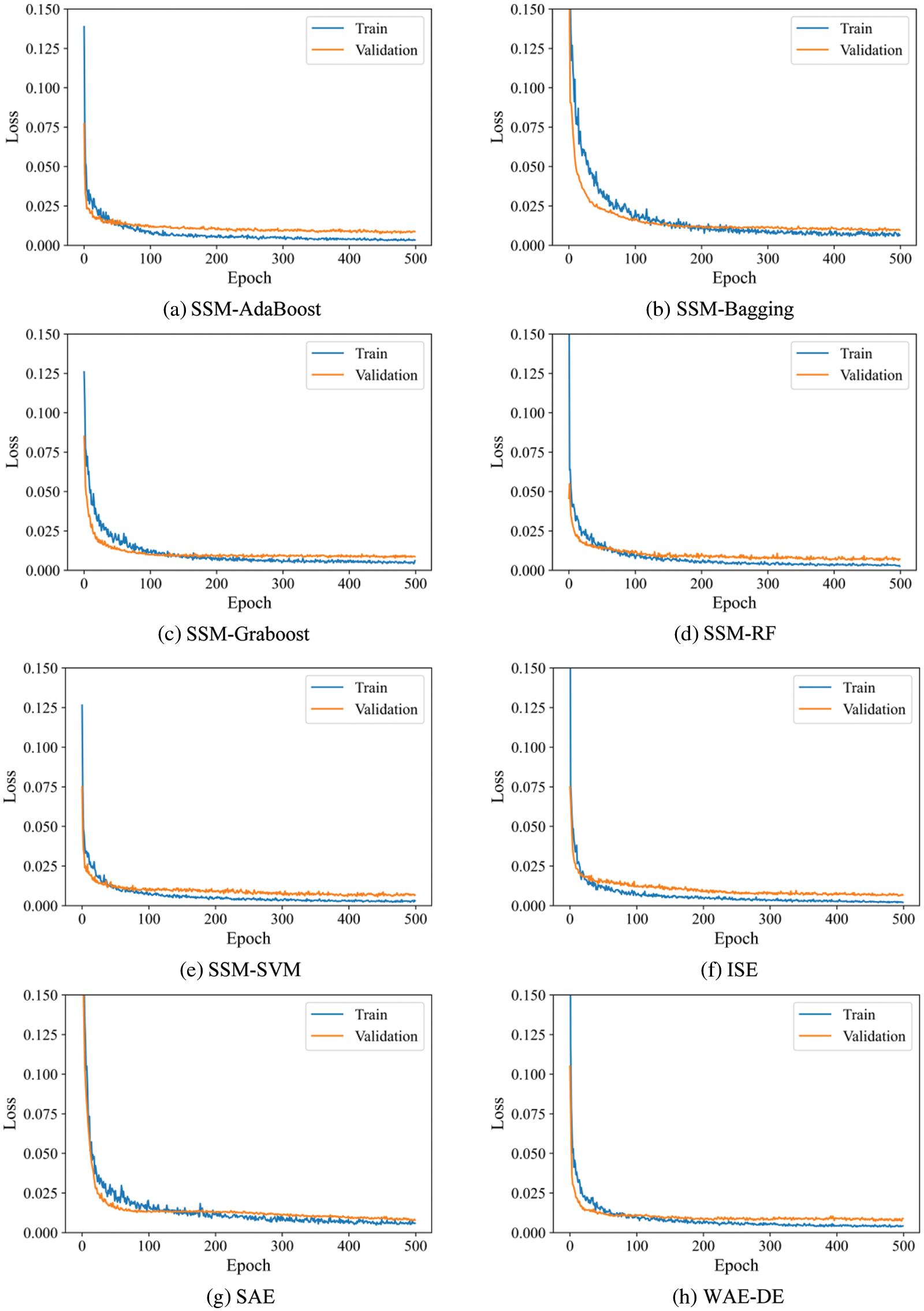
Figure 12: Loss-Epochs curve of various ensemble models
After a major earthquake, the timely success of a post-reconnaissance and recovery effort depends on the accurate assessment of inflicted structural damages. It is crucial to assess the seismic risk of structures in earthquake-prone areas and to collect data on the built domain within a possibly wide geographical area, following a severe earthquake. This paper developed and evaluated ensemble learning algorithms for identifying structural damage in RC members. The utilized ensemble algorithms include simple averaging, integrated stacking, separate stacking, and hybrid weighted averaging ensemble and differential evolution (WAE-DE) ensemble model, which are based on deep convolutional networks. The results were reported and examined using a confusion matrix, a table that was used to assess algorithm’s performance. Overall accuracy, precision, and recall metrics are reported for each model.
The results show that the WAE-DE and separate stacking ensemble with support vector machine (SSM-SVM) had the highest accuracy in the testing phase. The prediction accuracy of the ensemble models with the performance of sub-models shows the efficiency of the SSM-SVM and WAE-DE models in classifying damage types of RC members. Furthermore, the results demonstrated that predicting flexural-shear damage was challenging, as the lowest value of the recall corresponded to this type of damage for the majority of the investigated cases. The results of the proposed models were compared with three well-known deep convolutional neuronal networks (benchmark) models, including VGG-16, VGG-19, and ResNet-50 models. The benchmark models were significantly poorer than the of the ensemble models in terms of performance. The best benchmark model (VGG-19) had an accuracy of 72%, but the SSM-SVM and WAE-DE models had an accuracy of 94%. Because the WAE-DE and SSM-SVM models have the highest accuracy, precision, and recall among the various ML models, these two algorithms are recommended as the best prediction models for detecting structural damage.
Data Availability: Some or all data, models, or code that support the findings of this study are available from the corresponding author upon reasonable request.
Funding Statement: The authors received no specific funding for this study.
Conflicts of Interest: The authors declare that they have no conflicts of interest to report regarding the present study.
References
1. Zhang, J., Jin, Y., Sun, B., Han, Y., Hong, Y. (2021). Study on the improvement of the application of complete ensemble empirical mode decomposition with adaptive noise in hydrology based on RBFNN data extension technology. Computer Modeling in Engineering & Sciences, 126(2), 755–770. DOI 10.32604/cmes.2021.012686. [Google Scholar] [CrossRef]
2. Hassanpour, M., Malek, H. (2020). Learning document image features with SqueezeNet convolutional neural network. International Journal of Engineering, 33(7), 1201–1207. DOI 10.5829/ije.2020.33.07a.05. [Google Scholar] [CrossRef]
3. Ko, Y. F., Ju, J. W. W. (2021). Effective elastic properties of 3-phase particle reinforced composites with randomly dispersed elastic spherical particles of different sizes. Computer Modeling in Engineering & Sciences, 129(3), 1305–1328. DOI 10.32604/cmes.2021.017589. [Google Scholar] [CrossRef]
4. Es-haghi, M. S., Barkhordari, M. S., Huang, Z., Ye, J. (2022). Multicriteria decision-making methods in selecting seismic upgrading strategy of high-rise RC wall buildings. Journal of Structural Engineering, 148(4), 04022015. DOI 10.1061/(ASCE)ST.1943-541X.0003304. [Google Scholar] [CrossRef]
5. Naser, M., Kodur, V., Thai, H. T., Hawileh, R., Abdalla, J. et al. (2021). StructuresNet and FireNet: Benchmarking databases and machine learning algorithms in structural and fire engineering domains. Journal of Building Engineering, 44, 102977. DOI 10.1016/j.jobe.2021.102977. [Google Scholar] [CrossRef]
6. Han, Z., Chen, H., Liu, Y., Li, Y., Du, Y. et al. (2021). Vision-based crack detection of asphalt pavement using deep convolutional neural network. Iranian Journal of Science and Technology, Transactions of Civil Engineering, 45, 1–9. DOI 10.1007/s40996-021-00668-x. [Google Scholar] [CrossRef]
7. Murlidhar, B. R., Nguyen, H., Rostami, J., Bui, X., Armaghani, D. J. et al. (2021). Prediction of flyrock distance induced by mine blasting using a novel harris hawks optimization-based multi-layer perceptron neural network. Journal of Rock Mechanics and Geotechnical Engineering, 13(6), 1413–1427. DOI 10.1016/j.jrmge.2021.08.005. [Google Scholar] [CrossRef]
8. Liu, J. C., Huang, L., Chen, Z., Ye, H. (2021). A comparative study of artificial intelligent methods for explosive spalling diagnosis of hybrid fiber-reinforced ultra-high-performance concrete. International Journal of Civil Engineering, 1–22. DOI 10.1007/s40999-021-00689-7. [Google Scholar] [CrossRef]
9. Zawad, M., Zawad, M., Rahman, M., Priyom, S. (2021). A comparative review of image processing based crack detection techniques on civil engineering structures. Journal of Soft Computing in Civil Engineering, 5(3), 58–77. DOI 10.22115/SCCE.2021.287729.1325. [Google Scholar] [CrossRef]
10. Hammal, S., Bourahla, N., Laouami, N. (2020). Neural-network based prediction of inelastic response spectra. Civil Engineering Journal, 6(6), 1124–1135. DOI 10.28991/cej-2020-03091534. [Google Scholar] [CrossRef]
11. Amini, A., Kia, M., Bayat, M. (2021). Seismic vulnerability macrozonation map of SMRFs located in Tehran via reliability framework. Structural Engineering and Mechanics, 78(3), 351–368. DOI 10.12989/sem.2021.78.3.351. [Google Scholar] [CrossRef]
12. Gupta, S. K., Das, S. (2021). Damage detection in a cantilever beam using noisy mode shapes with an application of artificial neural network-based improved mode shape curvature technique. Asian Journal of Civil Engineering, 22(8), 1671–1693. DOI 10.1007/s42107-021-00404-w. [Google Scholar] [CrossRef]
13. Das, A. K., Leung, C. K., Wan, K. T. (2021). Application of deep convolutional neural networks for automated and rapid identification and computation of crack statistics of thin cracks in strain hardening cementitious composites (SHCCs). Cement and Concrete Composites, 122, 104159. DOI 10.1016/j.cemconcomp.2021.104159. [Google Scholar] [CrossRef]
14. Abdelkader, E. M. (2021). On the hybridization of pre-trained deep learning and differential evolution algorithms for semantic crack detection and recognition in ensemble of infrastructures. Smart and Sustainable Built Environment. DOI 10.1108/SASBE-01-2021-0010. [Google Scholar] [CrossRef]
15. Reis, H. C., Khoshelham, K. (2021). ReCRNet: A deep residual network for crack detection in historical buildings. Arabian Journal of Geosciences, 14(20), 1–13. DOI 10.1007/s12517-021-08491-4. [Google Scholar] [CrossRef]
16. Wan, H., Gao, L., Su, M., Sun, Q., Huang, L. (2021). Attention-based convolutional neural network for pavement crack detection. Advances in Materials Science and Engineering, 2021. DOI 10.1155/2021/5520515. [Google Scholar] [CrossRef]
17. Bigdeli, N., Jabbari, H., Shojaei, M. (2021). An intelligent method for crack classification in concrete structures based on deep neural networks. Amirkabir Journal of Civil Engineering, 53(8), 3–3. DOI 10.22060/ceej.2020.17738.6660. [Google Scholar] [CrossRef]
18. Mohammed, M. A., Han, Z., Li, Y. (2021). Exploring the detection accuracy of concrete cracks using various CNN models. Advances in Materials Science and Engineering, 2021. DOI 10.1155/2021/9923704. [Google Scholar] [CrossRef]
19. Ye, X. W., Jin, T., Li, Z., Ma, S., Ding, Y. et al. (2021). Structural crack detection from benchmark data sets using pruned fully convolutional networks. Journal of Structural Engineering, 147(11), 04721008. DOI 10.1061/(ASCE)ST.1943-541X.0003140. [Google Scholar] [CrossRef]
20. Flah, M. (2020). Classification, localization, and quantification of structural damage in concrete structures using convolutional neural networks (Electronic Thesis and Dissertation). https://ir.lib.uwo.ca/etd/7188. [Google Scholar]
21. Wang, X., Shahzad, M. M. (2021). A novel structural damage identification scheme based on deep learning framework. Structures, 29, 1537–1549. DOI 10.1016/j.istruc.2020.12.036. [Google Scholar] [CrossRef]
22. Meng, M., Zhu, K., Chen, K., Qu, H. (2021). A modified fully convolutional network for crack damage identification compared with conventional methods. Modelling and Simulation in Engineering, 2021. DOI 10.1155/2021/5298882. [Google Scholar] [CrossRef]
23. Quqa, S., Martakis, P., Movsessian, A., Pai, S., Reuland, Y. et al. (2021). Two-step approach for fatigue crack detection in steel bridges using convolutional neural networks. Journal of Civil Structural Health Monitoring, 12, 1–14. DOI 10.1007/s13349-021-00537-1. [Google Scholar] [CrossRef]
24. Sharma, S., Sen, S. (2020). One-dimensional convolutional neural network-based damage detection in structural joints. Journal of Civil Structural Health Monitoring, 10(5), 1057–1072. DOI 10.1007/s13349-020-00434-z. [Google Scholar] [CrossRef]
25. Sony, S. (2021). Bridge damage identification using deep learning-based convolutional neural networks (CNNs). Civil and Environmental Engineering Publications. https://ir.lib.uwo.ca/civilpub/203. [Google Scholar]
26. Alazzawi, O., Wang, D. (2021). Damage identification using the PZT impedance signals and residual learning algorithm. Journal of Civil Structural Health Monitoring, 11(5), 1225–1238. DOI 10.1007/s13349-021-00505-9. [Google Scholar] [CrossRef]
27. Yang, K., Ding, Y., Sun, P., Jiang, H., Wang, Z. (2021). Computer vision-based crack width identification using F-CNN model and pixel nonlinear calibration. Structure and Infrastructure Engineering, 1–12. DOI 10.1080/15732479.2021.1994617. [Google Scholar] [CrossRef]
28. Chen, Q., Xie, Y., Ao, Y., Li, T., Chen, G. et al. (2021). A deep neural network inverse solution to recover pre-crash impact data of car collisions. Transportation Research Part C: Emerging Technologies, 126, 103009. DOI 10.1016/j.trc.2021.103009 [Google Scholar] [CrossRef]
29. Chen, G., Li, T., Chen, Q., Ren, S., Wang, C. et al. (2019). Application of deep learning neural network to identify collision load conditions based on permanent plastic deformation of shell structures. Computational Mechanics, 64(2), 435–449. DOI 10.1007/s00466-019-01706-2. [Google Scholar] [CrossRef]
30. Gao, Y., Mosalam, K. M. (2020). PEER Hub ImageNet: A large-scale multiattribute benchmark data set of structural images. Journal of Structural Engineering, 146(10), 04020198. DOI 10.1061/(ASCE)ST.1943-541X.0002745. [Google Scholar] [CrossRef]
31. Gao, Y., Mosalam, K. M. (2018). Deep transfer learning for image-based structural damage recognition. Computer-Aided Civil and Infrastructure Engineering, 33(9), 748–768. DOI 10.1111/mice.12363. [Google Scholar] [CrossRef]
32. Moehle, J. (2015). Seismic design of reinforced concrete buildings. New York City, USA: McGraw-Hill Education. [Google Scholar]
33. Sandler, M., Howard, A., Zhu, M., Zhmoginov, A., Chen, L. C. (2018). MobileNetV2: Inverted residuals and linear bottlenecks. Proceedings of the IEEE Conference on Computer Vision and Pattern Recognition, pp. 4510–4520. San Juan, PR, USA. DOI 10.1109/CVPR.2018.00474. [Google Scholar] [CrossRef]
34. Zoph, B., Vasudevan, V., Shlens, J., Le, Q. V. (2018). Learning transferable architectures for scalable image recognition. Proceedings of the IEEE Conference on Computer Vision and Pattern Recognition, pp. 8697–8710. San Juan, PR, USA. DOI 10.1109/CVPR.2018.00907. [Google Scholar] [CrossRef]
35. Yosinski, J., Clune, J., Bengio, Y., Lipson, H. (2014). How transferable are features in deep neural networks? arXiv preprint arXiv:1411.1792. [Google Scholar]
36. Weiss, K., Khoshgoftaar, T. M., Wang, D. (2016). A survey of transfer learning. Journal of Big Data, 3(1), 1–40. DOI 10.1186/s40537-016-0043-6. [Google Scholar] [CrossRef]
37. Barkhordari, M. S., Armaghani, D. J., Fakharian, P. (2022). Ensemble machine learning models for prediction of flyrock due to quarry blasting. International Journal of Environmental Science and Technology, DOI 10.1007/s13762-022-04096-w. [Google Scholar] [CrossRef]
38. Barkhordari, M. S., Tehranizadeh, M. (2021). Response estimation of reinforced concrete shear walls using artificial neural network and simulated annealing algorithm. Structures, 34, 1155–1168. DOI 10.1016/j.istruc.2021.08.053. [Google Scholar] [CrossRef]
39. Ahrari, A., Essam, D., (2022). An introduction to evolutionary and memetic algorithms for parameter optimization. Evolutionary and memetic computing for project portfolio selection and scheduling, pp. 37–63. Denmark: Springer. [Google Scholar]
40. Price, K., Storn, R. M., Lampinen, J. A., (2006). Differential evolution: A practical approach to global optimization. Berlin, Germany: Springer Science & Business Media. [Google Scholar]
41. Barkhordari, M. S., Armaghani, D. J., Sabri, M. M. S., Ulrikh, D. V., Ahmad, M. (2022). The efficiency of hybrid intelligent models in predicting fiber-reinforced polymer concrete interfacial-bond strength. Materials, 15(9), 3019. DOI 10.3390/ma15093019. [Google Scholar] [CrossRef]
42. Patil, S., Patil, A., Phalle, V. M. (2018). Life prediction of bearing by using adaboost regressor. Proceedings of TRIBOINDIA--2018 An International Conference on Tribology, Faridabad Haryana, India, https://dx.doi.org/10.2139/ssrn.3398399. [Google Scholar]
43. Zhou, Z. H. (2019). Ensemble methods: Foundations and algorithms. New York, USA: Chapman and Hall/CRC. [Google Scholar]
44. Kumar, A., Mayank, J., (2020). Ensemble learning for AI developers. Berkeley, USA: Apress, Springer. [Google Scholar]
45. Michelucci, U., (2018). Applied deep learning—A case-based approach to understanding deep neural networks. New York, NY, USA: Apress Media. [Google Scholar]
46. Barkhordari, M. S., Tehranizadeh, M., Scott, M. H. (2021). Numerical modelling strategy for predicting the response of reinforced concrete walls using timoshenko theory. Magazine of Concrete Research, 73(19), 988–1010. DOI 10.1680/jmacr.19.00542. [Google Scholar] [CrossRef]
47. Barkhordari, M. S., Feng, D. C., Tehranizadeh, M. (2022). Efficiency of hybrid algorithms for estimating the shear strength of deep reinforced concrete beams. Periodica Polytechnica Civil Engineering, 66, 398–410. DOI 10.3311/PPci.19323. [Google Scholar] [CrossRef]
48. Brownlee, J., (2018). Better deep learning: Train faster, reduce overfitting, and make better predictions. Machine Learning Mastery. [Google Scholar]
49. Gao, Y., Mosalam, K. M., (2019). PEER Hub ImageNet: A large-scale multiattribute benchmark data set of structural images. PEER Report No.2019/07. University of California, Berkeley, CA: Pacific Earthquake Engineering Research Center. [Google Scholar]
50. Simonyan, K., Zisserman, A. (2014). Very deep convolutional networks for large-scale image recognition. arXiv preprint arXiv:1409, 1556. [Google Scholar]
51. He, K., Zhang, X., Ren, S., Sun, J. (2016). Deep residual learning for image recognition. Proceedings of the IEEE Conference on Computer Vision and Pattern Recognition, pp. 770–778. San Juan, PR, USA. [Google Scholar]
52. Brownlee, J. (2016). Machine learning mastery with python, vol. 527, pp. 100–120. Machine Learning Mastery Pty, Ltd. [Google Scholar]
Cite This Article
 Copyright © 2023 The Author(s). Published by Tech Science Press.
This work is licensed under a Creative Commons Attribution 4.0 International License , which permits unrestricted use, distribution, and reproduction in any medium, provided the original work is properly cited.
 Downloads
 Citation Tools