Optimizing Big Data Retrieval and Job Scheduling Using Deep Learning Approaches

1  Introduction

In recent years, the rapid growth of the amount of data coupled with the declining cost of storage equipment, the evolution of software technology, and the maturity of the cloud environment led to the rapid development of big data analytics [1]. When the amount of data is enormous, and the speed of data flow is fast, traditional methods are no longer for dealing with data storage, computing, and analysis in time, and excessively large-scale access will also cause I/O severe delay in a system. Faced with such explosive growth of large amounts of data, implementing tremendous distributed computing [2] with large-scale data clustering and type of not-only-SQL (NoSQL) storage technology has become a popular solution in recent years. Apache Hadoop or Spark [3] is currently the most widely known big data analytics platform in business intelligence with decentralized computing capabilities. Each of them is very suitable for typical extract-transform-load (ETL) workloads [4] due to its large-scale scalability and relatively low cost. Hadoop uses first-in-first-out (FIFO) [5] scheduling by default to prioritize jobs in the order in which they arrive. Although this kind of scheduling is relatively fair, it is likely to cause low system throughput. On the other hand, the response time of data retrieval using a traditional decentralized system is lengthy, causing inefficient job execution. Therefore, how to improve the efficiency of data retrieval and job scheduling becomes a crucial issue of big data analytics in business intelligence.

In terms of artificial intelligence development, deep learning [6] has rapidly developed in recent years. AlphaGo [7], developed by Google DeepMind in London, UK, defeated many Go masters in 2014. AI has become a hot research topic once again. The use of machine learning [8] or deep learning in various aspects of research and related applications is constantly prosperous. IBM developed a novel deep learning technology that mimics the working principle of the human brain, which can significantly reduce the speed of processing a large amount of data. Deep learning is a branch of artificial intelligence, and today’s technology giants Facebook, Amazon, and Google focus on its related development for many innovations. In this era, the explosive growth of data will exist, and how to process and analyze a large amount of data effectively has become an important topic.

Nowadays, data retrieval and job scheduling research mainly focuses on using Hadoop and Spark open-source big data platforms in business intelligence systems to improve efficiency. Generally speaking, this study considers encoding and indexing technologies to realize fast data retrieval to increase the system throughput in big data analytics. Developing high-performance job scheduling in big data analytics reduces the time of job waiting for execution in a queue. The objective of this paper is to develop an advanced deep learning model together with a high-performed indexing engine that can beat the previous method, integrating deep autoencoder [9] (DAE) and Solr indexing [10] (abbreviated DAE-SOLR), over the speed of big data retrieval significantly. Based on deep learning model, this paper explored integrating stacked sparse autoencoder (SSAE) [11] and Elasticsearch indexing [12], abbreviated SSAE-ES, to create a fast approach of data searching and distributed indexing, which can reduce the search scope of the database and dramatically speeds up data searching. Implementing the proposed SSAE-ES can outperform the previous method DAE-SOLR with higher data retrieval efficiency and system throughput for big data analytics in business intelligence. On the other hand, this paper tried to exploit deep neural networks (DNN) [13] to predict the approximate execution time of jobs and give prioritized job scheduling based on the shortest job first (SJF) [14], which can reduce the average waiting time of job execution and average weighted turnaround time [15].

2  Related Work

2.1 Literature Review

The real-time data processing and analysis are getting higher and higher for big data analytics in business intelligence. To pursue better performance of data analysis, the job schedule plays a vital role in improving the performance of big data analytics. For example, Yeh et al. [16] proposed the user can dynamically assign priorities for each job to speed up the execution speed of the job. However, it lacks automatic functions to get the job started and must get permission from the user every time. Thangaselvi et al. [17] mentioned the user could import self-adaptive MapReduce (SAMR) algorithm into Hadoop, which can adjust the parameters recalling the historical information saved on each node, thereby dynamically finding slow jobs. But SAMR works based on the model established by K-means [18]. A K-means approach usually has specific assumptions about the data distribution, while DNN with hierarchical feature learning has no explicit assumptions about the data. Therefore, DNN can establish a more complex data distribution than K-means to get better prediction results.

Many studies even apply deep learning to the distributed computing nodes. For example, Marquez et al. [19] used the concept of deep cascade learning to combine Spark’s distributed computing using multi-layer perceptrons to build a model that can perform large-scale data analysis in a short time [20]. However, there will still be a longer waiting time for job execution due to this model’s, i.e., FIFO, lack of job scheduling optimization. Likewise, Lee et al. [21] gave data clustering with deep autoencoder and Solr indexing to significantly improve the query performance. However, the system lacks suitable job scheduling. Besides, Chang et al. [22] proposed the memory-sensitive heterogeneous early finish time (MSHEFT) algorithm for improving job scheduling. Unfortunately, when encountering the same size as data in the different jobs, it performs scheduling just like a FIFO, and nothing can be improved at all.

Nature-inspired optimization can give some searching advantages by using meta-heuristic-like approaches rather than deep learning models. L. Abualigah et al. proposed a novel population-based optimization method called Aquila Optimizer (AO) [23], which the Aquila’s behaviors have inspired nature while catching the prey. Abualigah et al. [24] proposed a novel nature-inspired meta-heuristic optimizer, called Reptile Search Algorithm (RSA), motivated by the hunting behavior of Crocodiles. Regarding the arithmetic optimization algorithm used for searching the target data, Abualigah et al. [25] presented a comprehensive survey of the Internet of Drones (IoD) and its applications, deployments, and integration. Integration of IoD includes privacy protection, security authentication, neural network, blockchain, and optimization based-method. Instead, Time-consuming will be a crucial problem about the cost when people consider meta-heuristic-like approaches or the arithmetic optimization algorithm for searching in significant data retrieval issues.

2.2 Encoder for Data Clustering

Deep autoencoder (DAE) is an unsupervised learning model of neural networks. Its model architecture includes two fully connected feedforward networks, called encoder and decoder, which perform compression and decompression. After training AE, the user reserves the encoder and can input the data into the encoder. The encoder outputs a point located in the three-dimensional space, as shown in Fig. 1. Three-dimensional space divides itself into eight quadrants according to the X, Y, and Z axes, and the quadrants numbering from 1∼8 are inserted into the last column of the table, as shown in Fig. 2.

Figure 1: Data set mapping to 3D coordinates

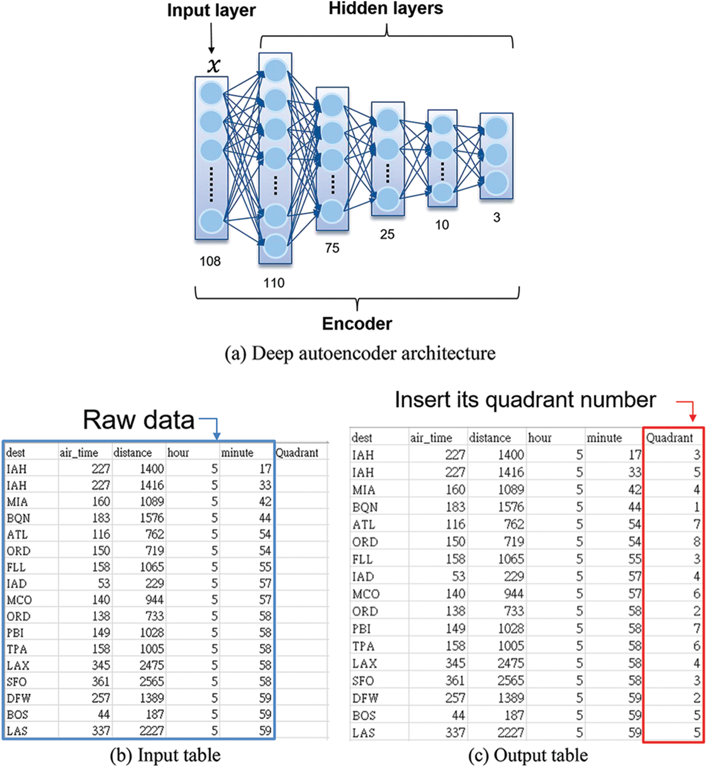
Figure 2: Encoder for data clustering

2.3 Stacked Sparse Autoencoder (SSAE)

Since training AE will activate the neurons of a hidden layer too frequently, AE may easily result in overfitting due to the degree of freedom being more considerable. A sparse constraint is added to the encoder part to reduce the number of activations of each neuron for every input signal. A specific input signal can only activate some neurons and will probably inactivate the others. In other words, each input signal of the sparse autoencoder cannot activate all of the neurons every time during the training phase, as shown in Fig. 3.

Figure 3: Sparse autoencoder model

The autoencoder with sparse constraints is called sparse autoencoder (SAE) [26]. SAE defines loss function on Eq. (1), where L represents the loss function without sparse constraint, KL stands for KL divergence [27], ρ denotes the expected activation degree of neurons in the network (if the activation function is a Sigmoid function, and SAE sets its value to 0.05, which means that most of the neural cell is not activated), and ρ^j is the average activation degree of the jth neuron. Here, people defined KL on Eq. (2) and use KL divergence to measure the similarity between the average activation output of hidden layer nodes and the sparsity ρ. Eq. (3) definds ρ^j the average activation degree on the training sample set in which m represents the number of training samples, and aj and xi stand for the response output of the jth node in the hidden layer to i samples.

Lsparse=L+β∑j⁡KL(ρ||ρ^j)(1)

KL(ρ||ρ^j)=ρlogρρ^j+(1−ρ)log1−ρ1−ρ^j(2)

ρ^j=\; ajm\; ∑i=1m⁡[xi](3)

After training multiple SAEs in which the user tuned each SAE layer by layer, the user finally stacked multiple SAEs up and called it stacked sparse autoencoder (SSAE), as shown in Fig. 4. The encoded output of the previous stage acts as the input of the next stage. After the training of the first SAE in Stage 1, the user can obtain the first hidden layer with m neurons denoted Hidden 1. Likewise, by cloning Hidden 1 to the second SAE in Stage 2, the user can obtain the second hidden layer with n neurons denoted Hidden 2. Finally, the user stacks two SAEs to form a stacked sparse autoencoder (SSAE). Based on the ahead of the hidden layer, the current hidden layer can generate a new set of features. Hopefully, the user can get more hidden layers according to layer-by-layer training in the different stages.

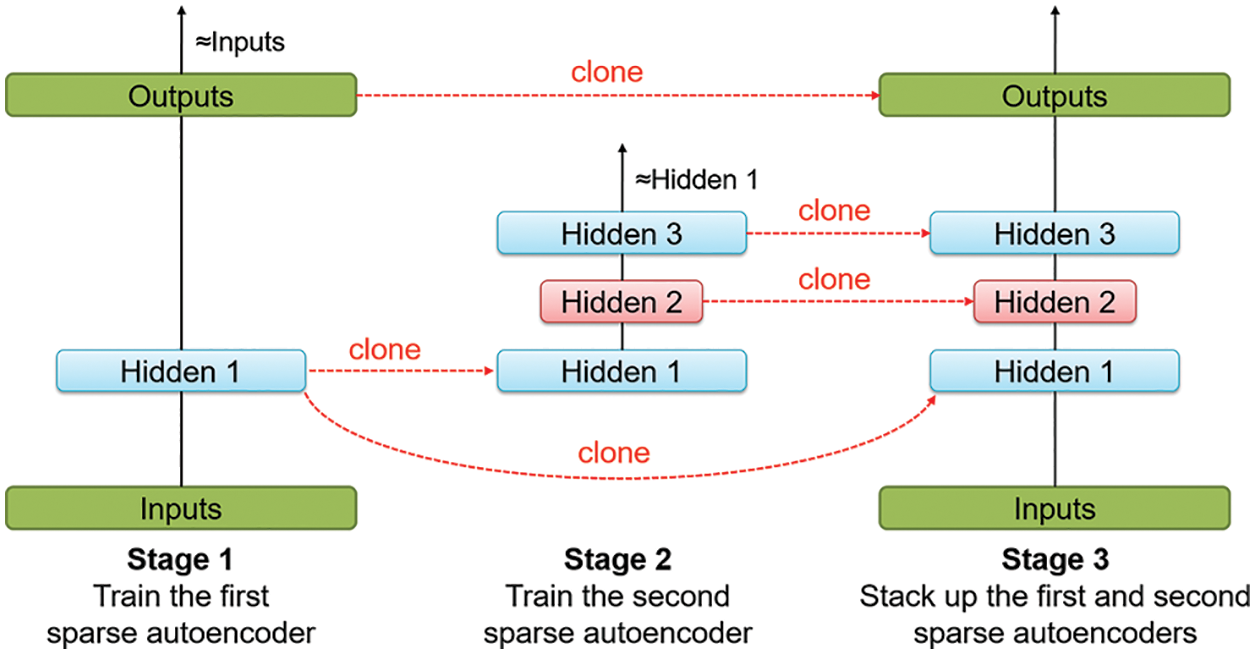
Figure 4: Layer-wise pre-training for two SAEs and stack them up

2.4 Data Retrieval by Indexing

According to the quadrant value of the last field, the data is divided into different files and then sent to Solr for data indexing. To cope with large-scale data retrieval, the longer it takes when the index volume is enormous, distributed indexes can speed up the search time. SolrCloud reduces the pressure of single-machine processing, and multiple servers need to complete indexing together. Its architecture is shown in Fig. 5.

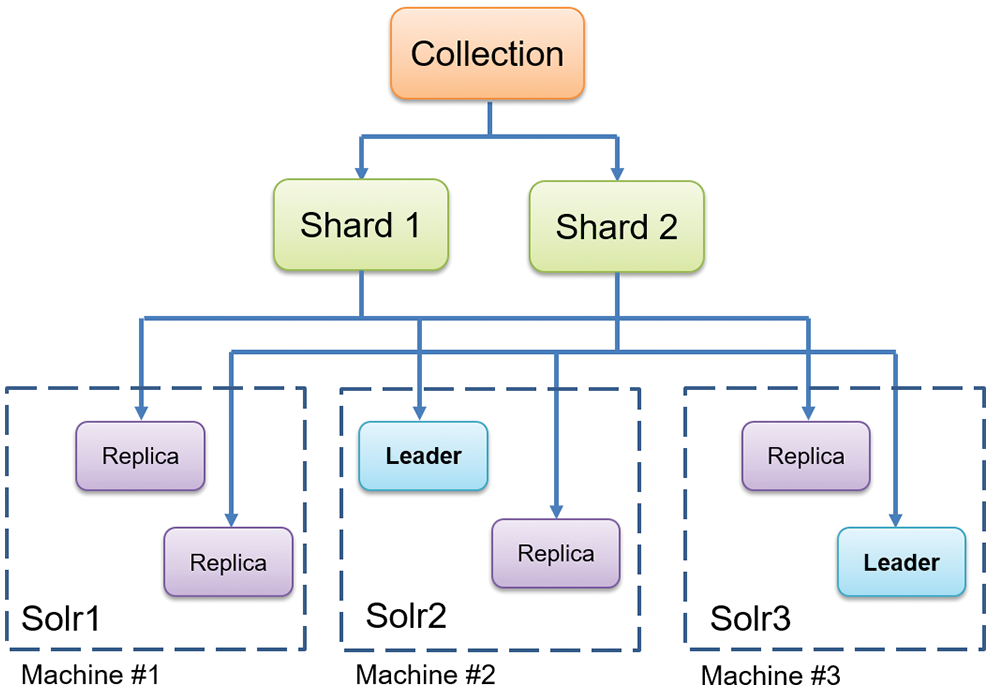
Figure 5: Solr architecture

After creating an index (collection) of data, Solr divided index into multiple shards, and each shard has a leader for job distribution, as shown in Fig. 6. When the replica completes the job, it will send the result back to the leader, and then the leader will send the result back to SolrCloud for the final result. The user can upload the file to any replica when the data is uploaded. If it is not the leader, it will forward the request to the leader of the same shard, and the leader will give the file path to each replica in the same shard. If the file does not belong to the same shard, the leader will transfer it to another leader in its corresponding shard. The corresponding leader will also give the file path to each replica in the same shard. The user manually uploaded the data to Solr after completing data clustering using the encoder process for subsequent node use. The flowchart of data preprocessing illustrates how to prepare the data clustering together with indexing, as shown in Fig. 7.

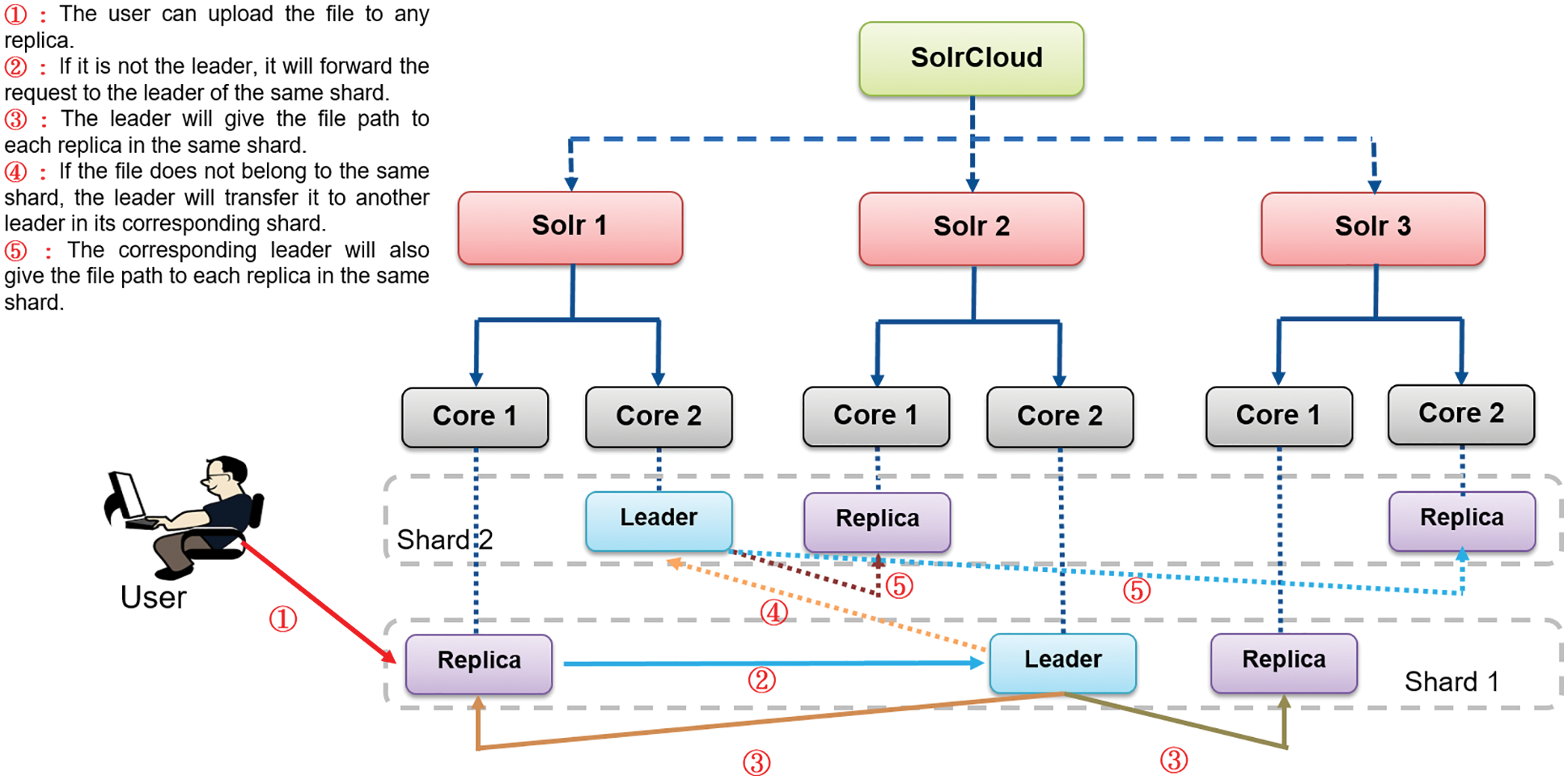
Figure 6: SolrCloud architecture

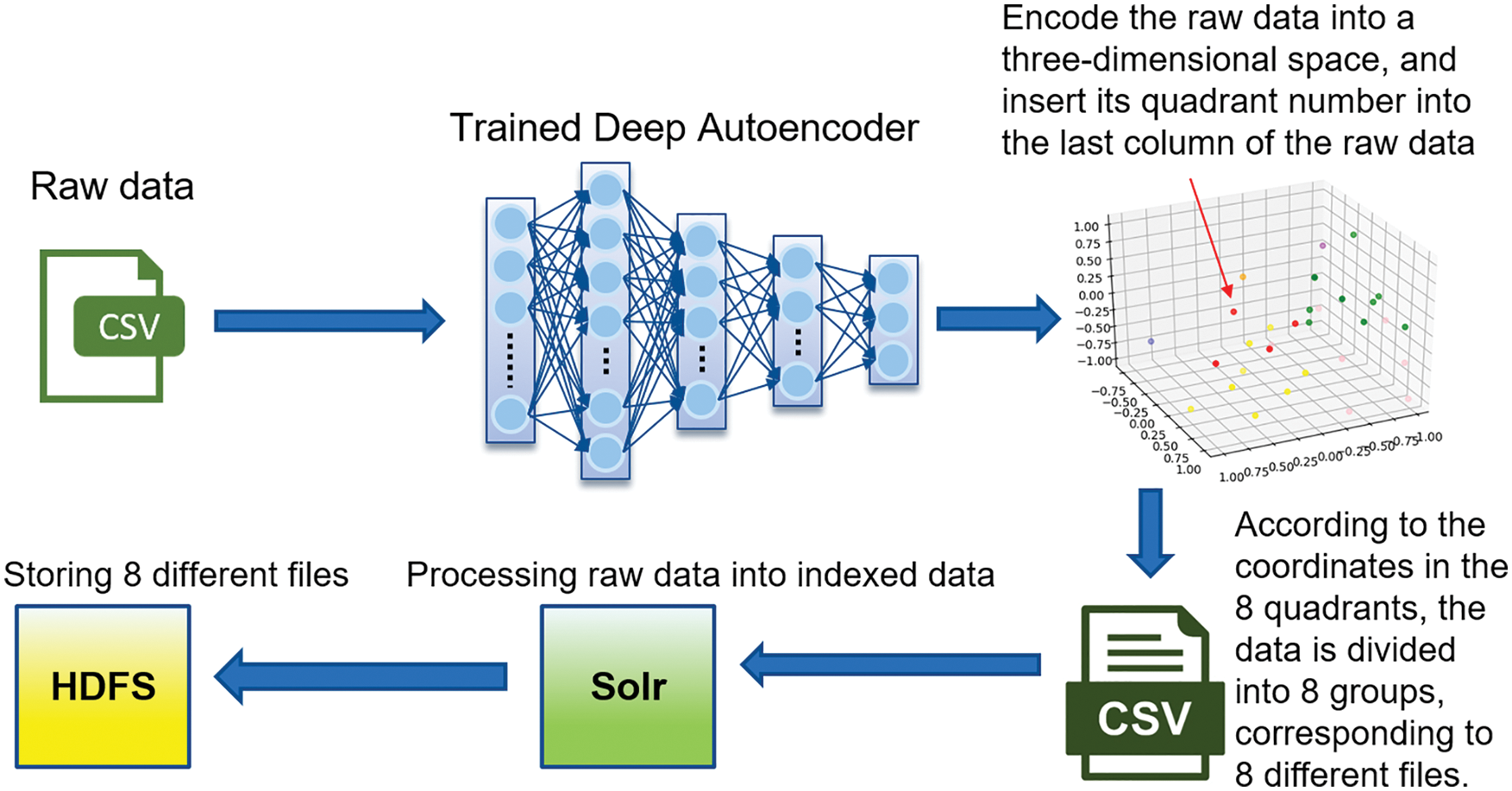
Figure 7: Data preprocessing flow

2.5 SQL Interface Selection

Developing an automatic SQL interface selection lets users choose an appropriate SQL interface [28], such as Hive, Impala, or SparkSQL, for performing SQL commands with the best efficiency. The appropriate SQL interface selection is valid according to the remaining memory size given in a cluster node. After trial and error, we found two critical points labeled as L1 and L2, where L1 represents the amount of memory around 5 GB and L2 10 GB. In this study, we set each node the amount of memory with 20 GB. Thus it defines three memory zones ranging from 0∼5 GB, 5 GB∼10 GB, and 10 GB∼20 GB, as shown in Fig. 8. When the remaining memory size is less than L1, the system will automatically select the Hive interface to perform SQL commands. The system will use the Impala interface between L1 and L2. If it is more than L2, the system will choose the SparkSQL interface, as shown in Fig. 8. We note that the Impala and SparkSQL interfaces need more memory to run the job having a large amount of data. Given sufficient memory, SparkSQL with in-memory computing capability can run the best efficiency in big data analytics. On the contrary, the Hive interface can run any job at a low level of memory size but is time-consuming.

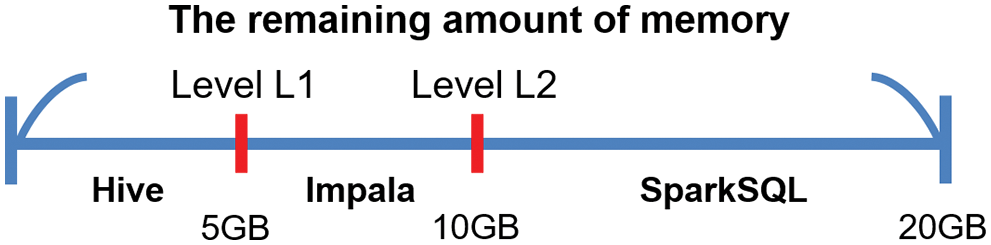
Figure 8: SQL interface selection

2.6 Job Scheduling Algorithm MSHEFT

Heterogeneous early finish time (HEFT) [29] is a heuristic way to schedule a set of dependent jobs onto a network of heterogeneous workers that takes communication time into account. HEFT works on a list out of the scheduling algorithm that establishes a priority list first. HEFT will assign each job to the appropriate CPU to follow the sorted priority list to complete the job as soon as possible. People modified the HEFT algorithm to the memory-sensitive heterogeneous early finish time (MSHEFT) algorithm [22] that first considers the job’s priority, then the data size, and, finally, the remaining memory size to choose the appropriate SQL command interface automatically. The flow chart of job processing with the MSHEFT algorithm and automatic SQL interface selection, as shown in Fig. 9.

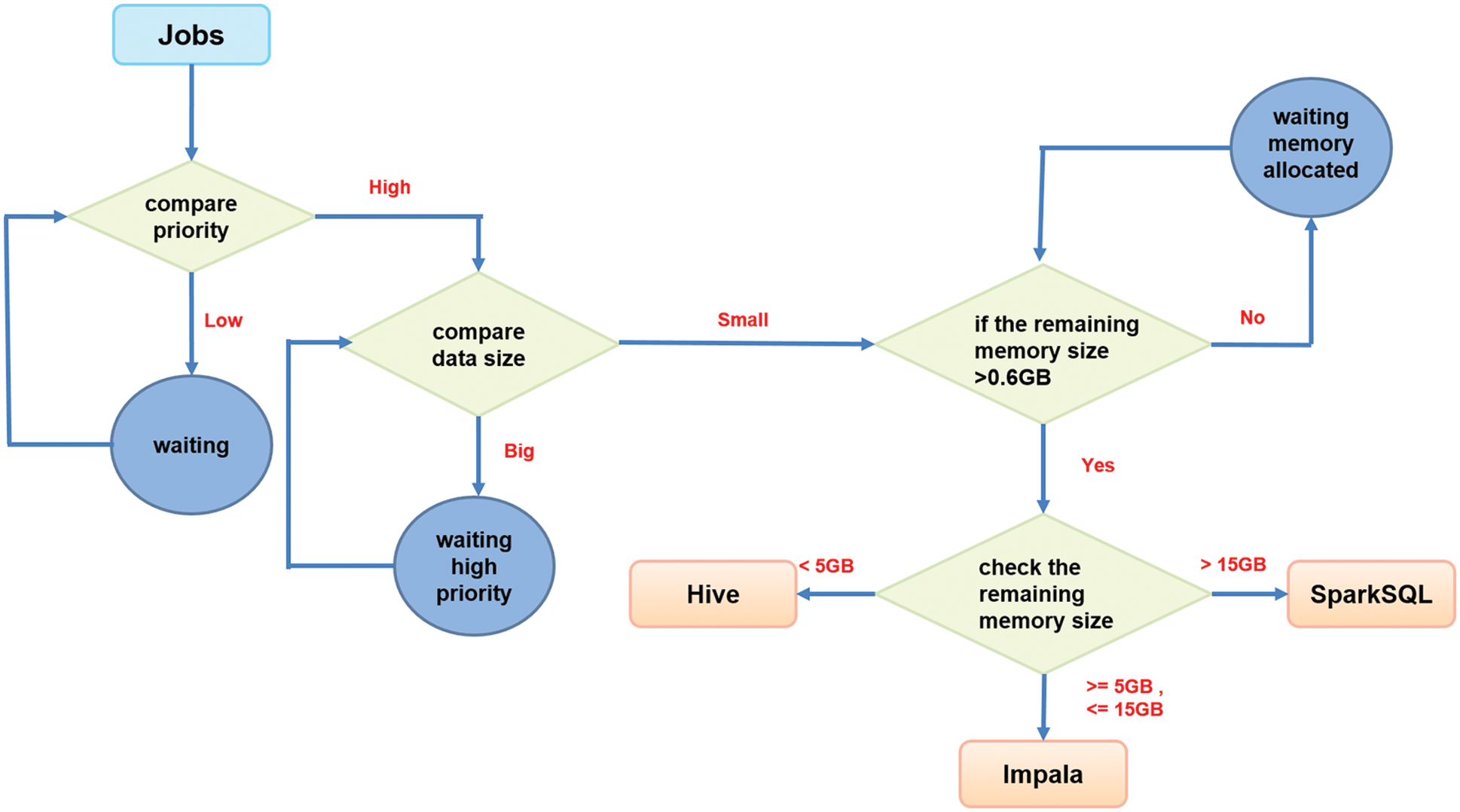
Figure 9: Job scheduling with MSHEFT algorithm and SQL interface selection

2.7 Two-Class Caching in Data Retrieval

Two-class caching is usually used to maximize the distributed system’s performance and optimize data retrieval and job scheduling. Two-class caching consists of in-memory and in-disk caches to save excessive hardware resource consumption caused by repeated searches. Two-class caching describes the flow in the following, as shown in Fig. 10.

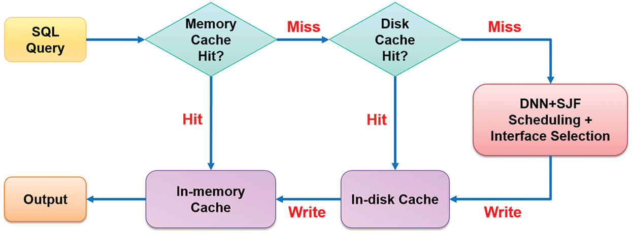
Figure 10: The flow of two-class caching in data retrieval

2.8 In-Memory Cache Mechanism

In terms of in-memory cache design, Memcached [30], a distributed high-speed fast memory system, temporarily stores data. Memcached can store the data in the memory in the form of key-value. A colossal hash table is constructed in the memory so that users can quickly query the corresponding data value through the key-value. Therefore, it is often used as a cache function to speed up the access performance of the system. However, the Memcached system has specific restrictions on its use. The default maximum length of the key-value is only 250 characters, and the acceptable storage data size cannot exceed 1 MB. Therefore, it is necessary first to divide and store the search results when storing the cache.

After the user enters the SQL command, the system will first use the MD5 algorithm [31] to convert the command into 16 bytes of hash value results and use the hash value as the unique identification code (i.e., key-value) for this search job, as shown in Fig. 11. If there is the exact SQL requirement later, it still results in the same hash value through the MD5 algorithm. The system can obtain the data through this unique identification code and realize the mechanism of cache design.

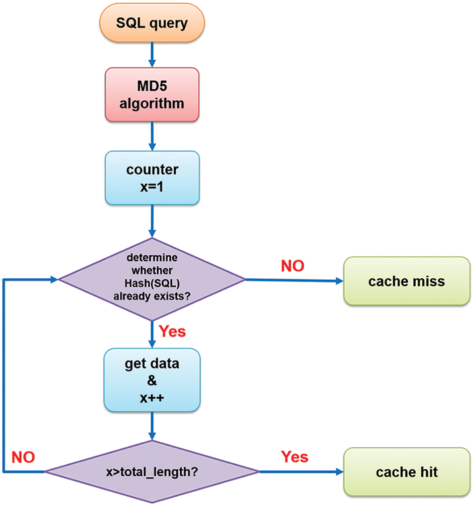
Figure 11: In-memory cache flow

2.9 In-Disk Cache Mechanism

As for in-disk, this paper uses HDFS distributed file system as the platform for in-disk cache storage. Since HDFS does not have storage capacity limitations like the Memcached system, it is only necessary to save a copy of the search result and upload it to HDFS. Similarly, the exact unique identification code as applied in the in-memory cache system names its file for identification, as shown in Fig. 12. Since files in HDFS will not become invalid automatically, users must periodically delete them manually in HDFS. Therefore, this paper also has the function of active clearance. The user only needs to enter the “purge x” command in the CLI, and the system can automatically delete the cache data that the user has not accessed within x days.

Figure 12: Cached files saving in HDFS

3  Method

3.1 Improved Big Data Analytics

In Fig. 13, improving the performance of big data analytics in a business intelligence system concerns three aspects: data retrieval, job scheduling, and different SQL command interfaces. The first one aims to speed up the data searching in big data. Therefore, this study must reduce the scope of data searching in the database and then implement data retrieval as fast as possible. This study introduced an approach to reduce the searching scope using data clustering with stacked sparse autoencoder, followed by a fast query response using quickly distributed data indexing with Elasticsearch, then stored tables into HDFS. The speed of data retrieval is relative to SQL command interfaces, so we will explore how to find the appropriate interface for the current situations of a node. This study has introduced three SQL command interfaces: Hive, Impala, and SparkSQL [28].

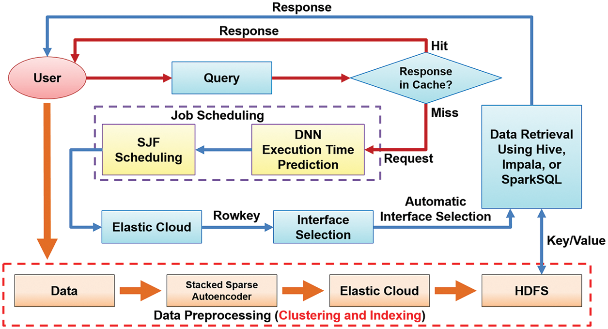
Figure 13: The optimization of big data analytics flow

On the other hand, the deep neural network carried out the time prediction of job execution to optimize job scheduling in big data analytics. According to the job with the shortest time for execution as the higher priority in scheduling, it can reduce the average waiting time in a queue. Finally, users only need to enter SQL commands through the Command-Line Interface (CLI), and the system will automatically detect the remaining memory size of a node and select the appropriate SQL interface to carry out the jobs, which can also speed up the job execution and is called the automatic interface selection. In particular, a SQL query can save the searching result into an in-memory or in-disk cache. Therefore, you can directly cache the data without launching the SQL command interfaces if you want to retrieve the same data repeatedly in a short time. The cache indeed speeds up the data retrieval dramatically.

3.2 Data Clustering by Mapping

The Stacked Sparse Autoencoder (SSAE) model can apply to a data set clustering. The dimensional vector of the SSAE input and output layers is the number of initial data columns denoted m. SSAE constructs the l-layer neurons as an encoder and the mirror layers as a decoder with unsupervised learning. The output of each layer is connected to the input of followed layer to reduce the data dimension and finally obtain an output of n-dimensional vector in the middle layer, and then run the decoder of an SSAE in reverse order to restore the initial input data column. There is an example of SSAE, as shown in Fig. 14. In Fig. 14, the loss function is MSE, the activation function is Sigmoid, and the optimizer is Adam.

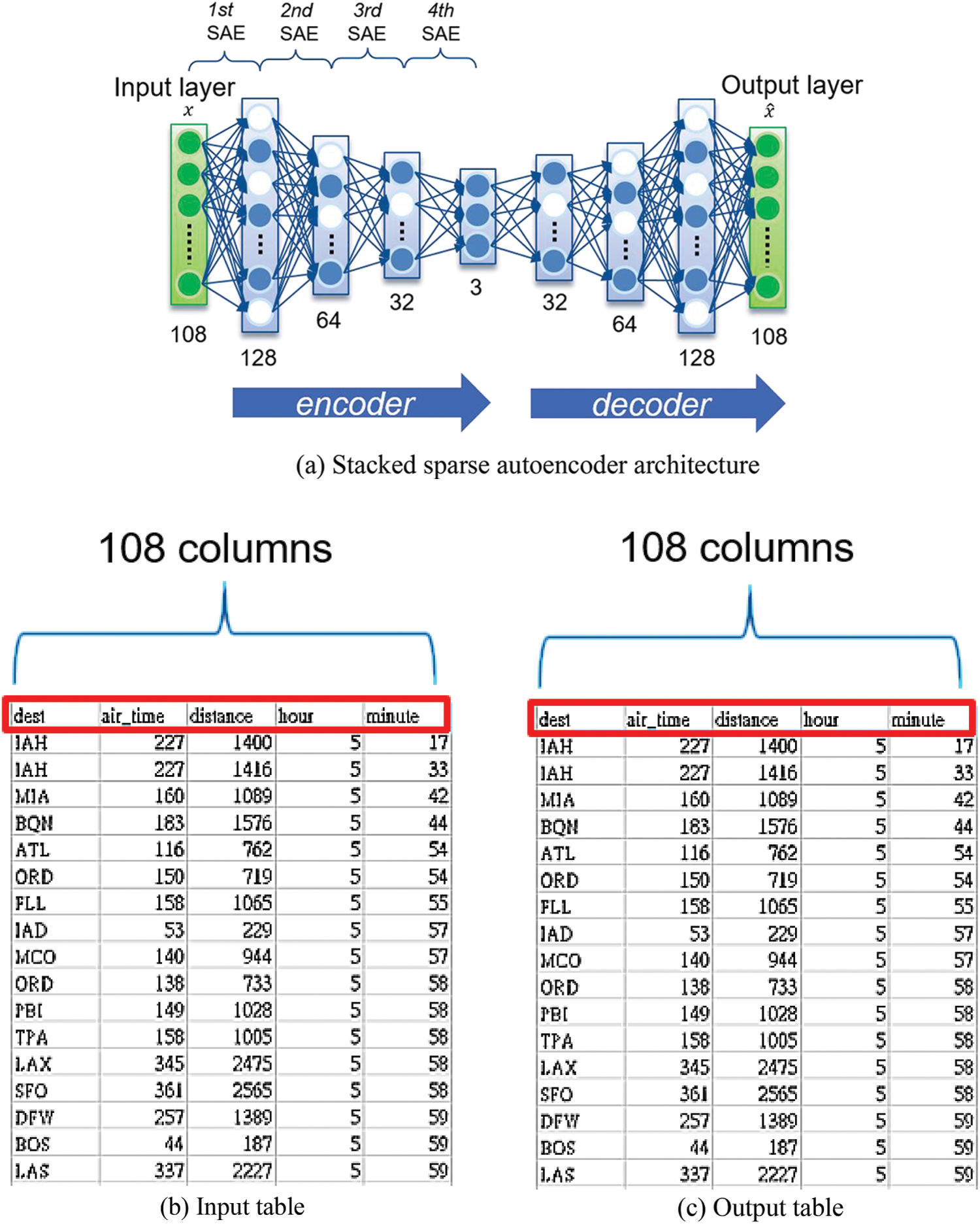
Figure 14: Data clustering using stacked sparse autoencoder

The results of running 50 epochs between AE and SSAE training show their visualized results in Fig. 15. Since AE does not have sparsity restriction, it turns out to be some of the different classes of data entangled around the same area, resulting in uneven data distribution and worse the effect of data clustering. In Fig. 15a, two data sets may be mapped to the same area and have entangled, where there is no apparent separation between the classes, such as gray-class tangled with purple-class, and red-class tangled with brown-class. The SSAE with sparse constraints can effectively solve this problem, making the sampled data of the same class closer and the separation between different classes more pronounced, as shown in Fig. 15b.

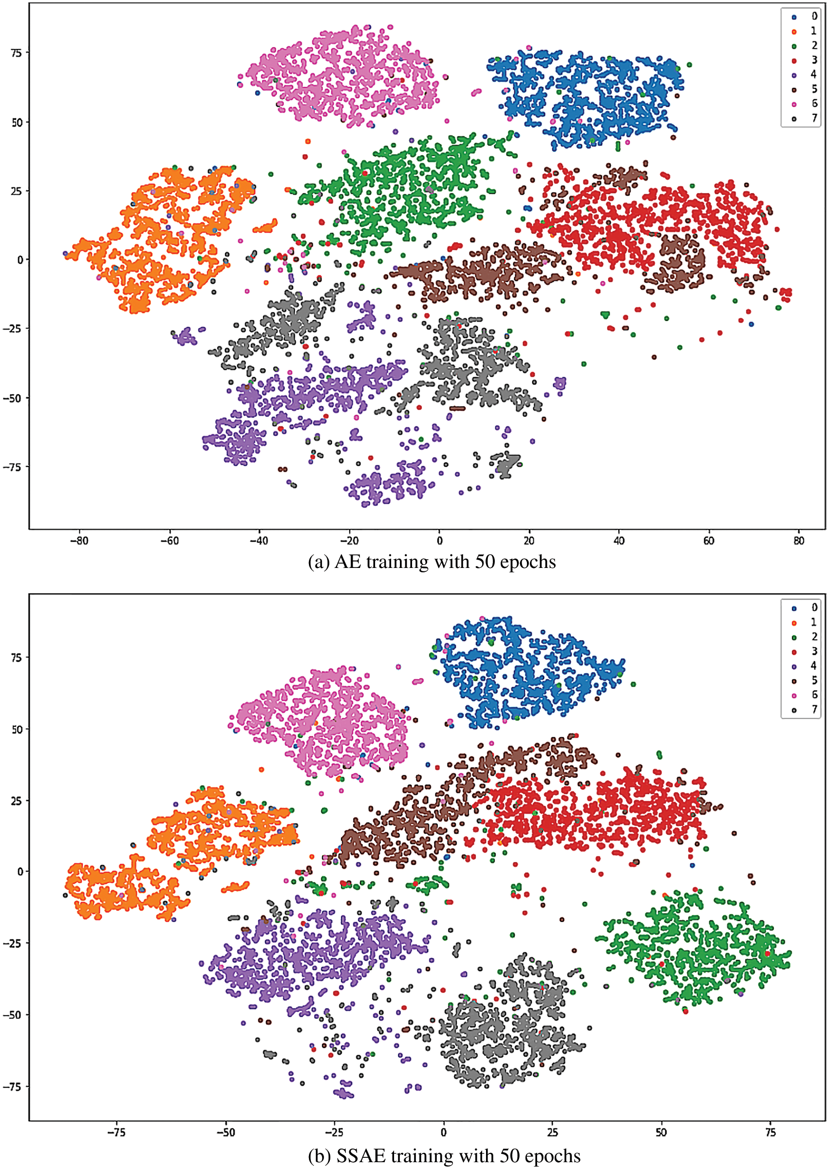
Figure 15: Data visualization results between AE and SSAE training

Here, we separate data into eight classes for a specific data set. Therefore, the output of the last hidden layer of the encoder from a trained SSAE model represents the mapping of each row of data to a point in the 3-dimensional space. According to the X, Y, and Z axes in the 3-dimensional space, SSAE automatically divided the data into eight classes. The corresponding eight quadrants numbering from 1 to 8 are inserted into the last column of the original data table, as shown in Figs. 1 and 2. In this study, the user applies the SSAE to data clustering instead of AE. After data clustering, the user can upload the tables to Elasticsearch for distributed indexing in them.

3.3 Data Retrieval by Quick Indexing

The system will generally spend longer I/O time to cope with large-scale data retrieval. Distributed indexing using Elasticsearch can speed up the data search speed and resolve the bottleneck problem about single-machine processing with time-consuming. Multi-server processing in a cluster can implement an indexing function to run the data search as fast as possible. When started each node, the system will automatically join this node and designate one of them to act as the master node. Accordingly, Elasticsearch, as shown in Fig. 16, indexed the data and then stored the data into the distributed file system HDFS.

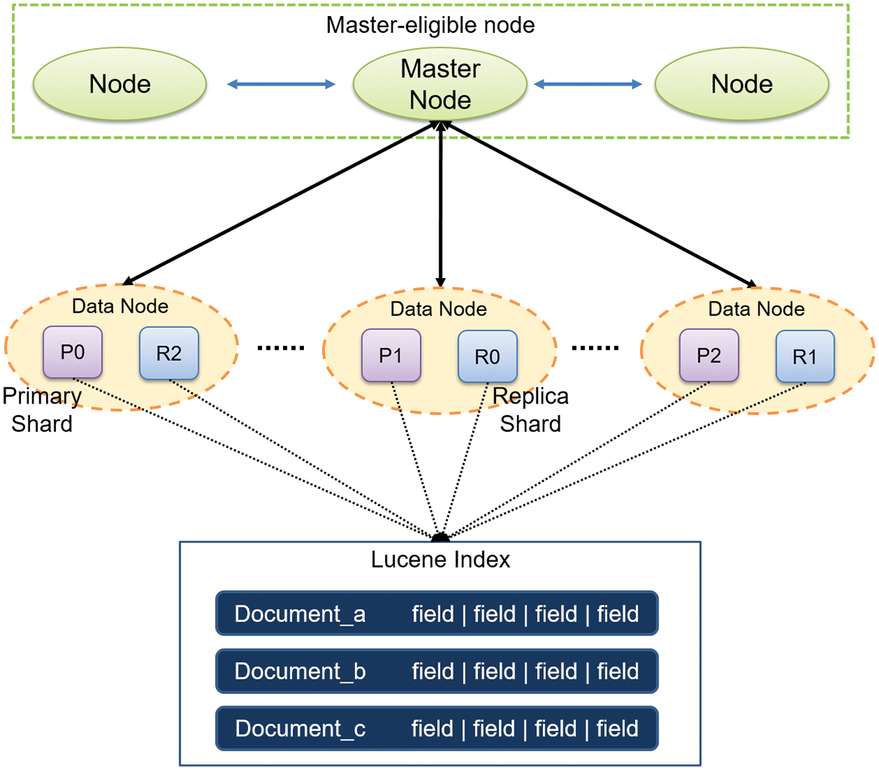
Figure 16: Cluster by Elasticsearch

After clustering input data into three-dimensional space, the user can manually upload this data set to Elasticsearch for distributed indexing, as shown in Fig. 17. When an input data set needs to be indexed, the indexing tool starts if the current node is the master node; otherwise, it will forward it to the master node. In Fig. 18, Elasticsearch first checks whether the data set was indexed before. If not, Elasticsearch will start building the index, write the results into the Lucene index, and use the hash algorithm to ensure that it makes indexed data evenly distributed and stored in the designated primary shard and replica shard. Meanwhile, Elasticsearch will create a corresponding version number and store it in translog. Elasticsearch supposes comparing the existing version numbers with the new ones to check any conflict if the data set is indexed early. If not, it can start indexing. If yes, Elasticsearch returns an error result that writes to translog. Finally, indexed data stored in HDFS can apply for the job with SQL command, as shown in Fig. 13.

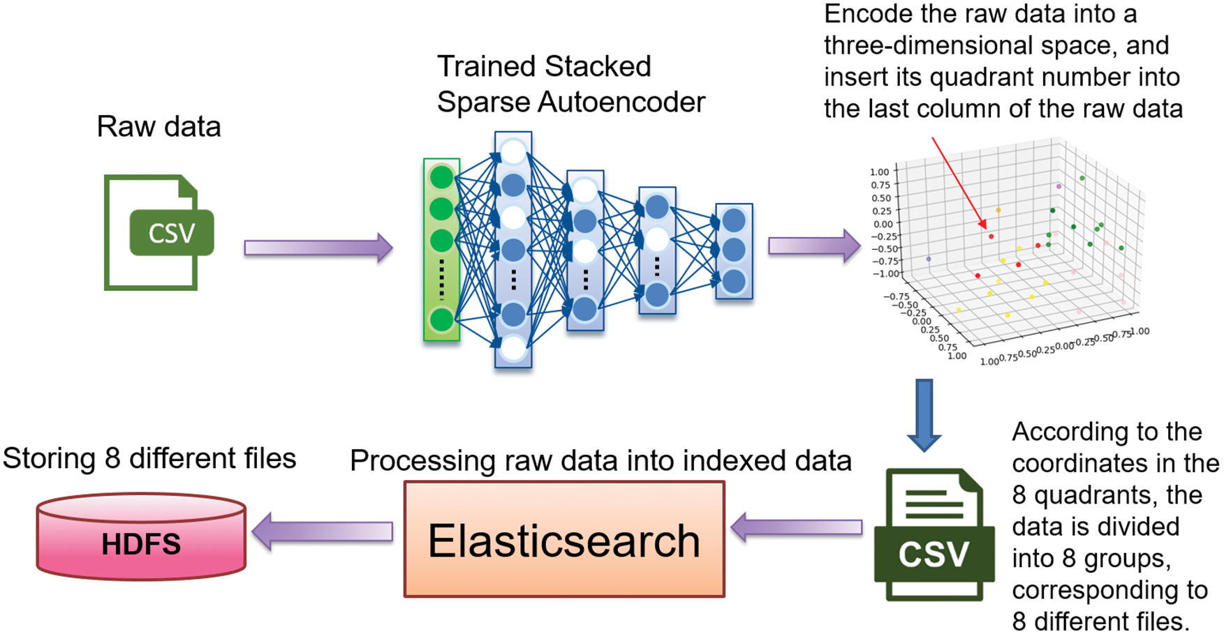
Figure 17: Data clustering and indexing flow

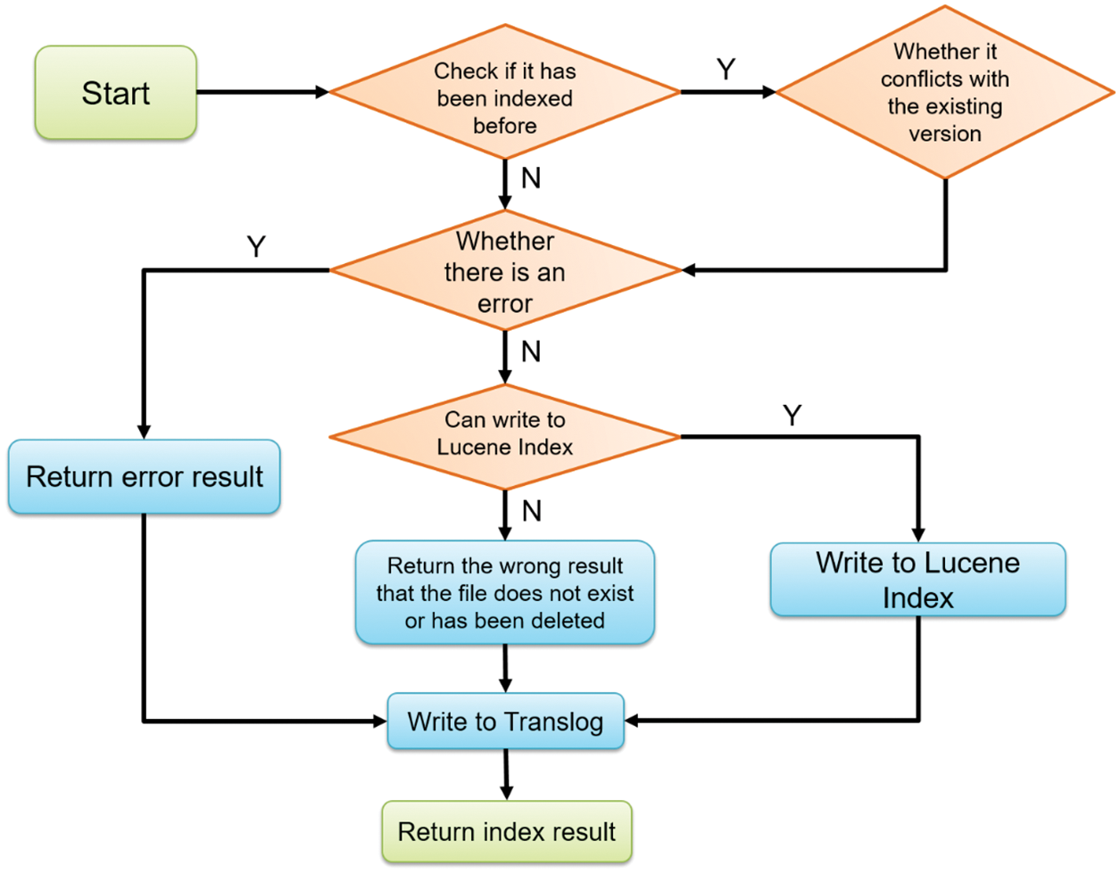
Figure 18: Indexing flow of Elasticsearch

3.4 Deep Neural Network Prediction for Job Scheduling Optimization

According to the SJF job scheduling algorithm, users can train a deep neural network (DNN) to predict the approximate job execution time. The input layer of this DNN has a six-dimensional vector, including data size, the number of data rows, the number of data columns, the time complexity of program execution, the SQL interface environment, and the remaining memory size. The output layer has only a one-dimensional vector (Label) as a time prediction of performing data retrieval, as shown in Fig. 19. Users can collect real data from the web to train a DNN model. Three sets of SQL interfaces—Hive, Impala, and SparkSQL—are used to test a DNN time prediction applied to the data retrieval function under the different remaining memory sizes given. The activation function in a DNN is ReLU, the loss function MSE, and the optimizer Adam [32]. We will give the DNN model architecture and loss curve during the training, as shown in Figs. 20 and 21, respectively.

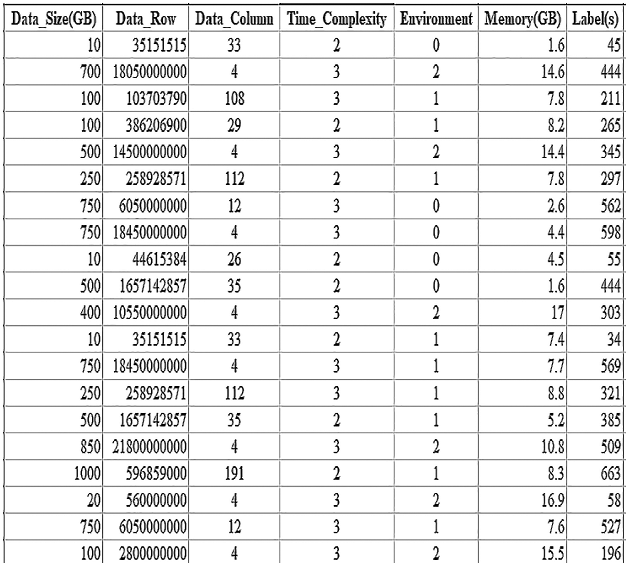
Figure 19: Column “Label(s)” indicating the output of a deep neural network (DNN)

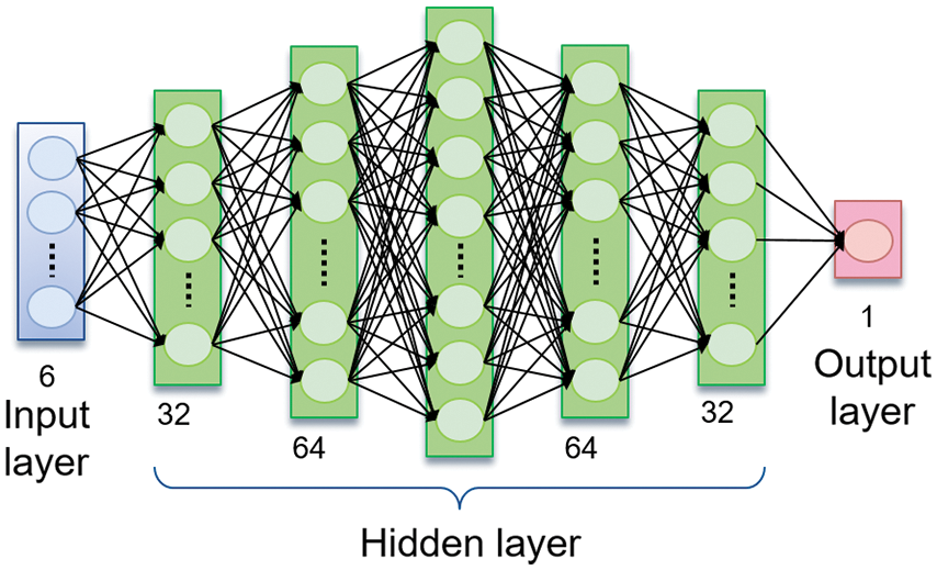
Figure 20: Deep neural network (DNN) architecture

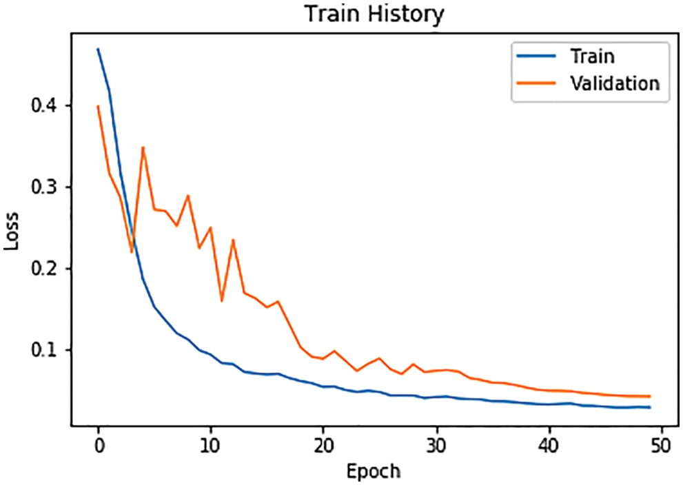
Figure 21: Loss curve during DNN training phase

In addition, we used a combination of deep neural network prediction and the shortest job priority scheduling to optimize the job scheduling. When a job enters the queue, the system first considers its execution priority and then predicts its approximate execution time to view as a job scheduling condition. Finally, the system will consider the remaining memory size to select the appropriate SQL interface to carry out the input SQL command. In such a way, the system can implement the significant throughput. Fig. 22 describes the flow of the proposed method mentioned above.

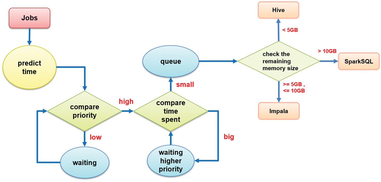
Figure 22: The flow of job scheduling optimization

3.5 Execution Commends and Its Flow

The designed programs in this study contain many application functions. Users can issue commands through the command-line interface (CLI) to input SQL commands. All commands of the programs describe their functions, as listed in Table 1. Fig. 23 gives the execution flow.

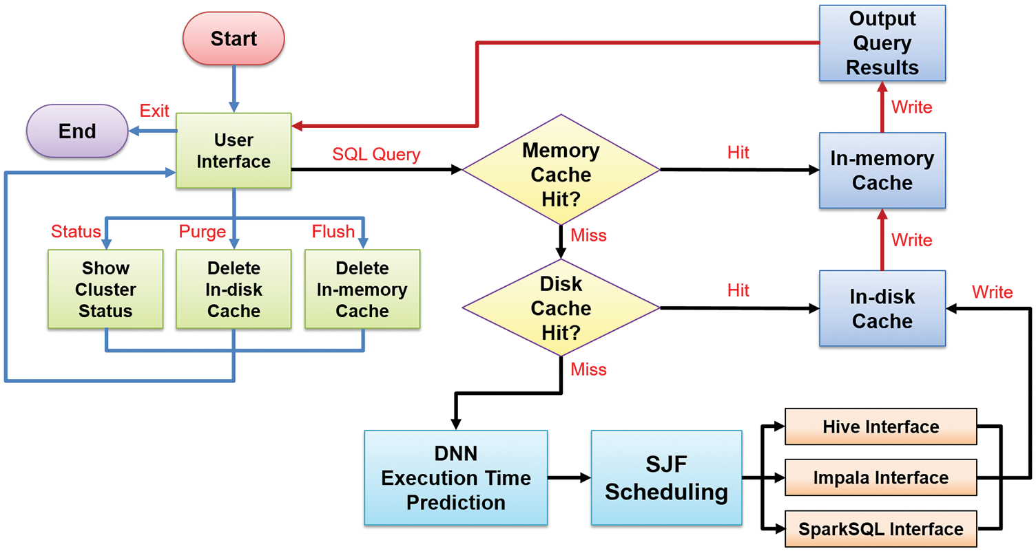
Figure 23: Job execution flow

4  Experiment Results and Discussion

4.1 Experimental Environment

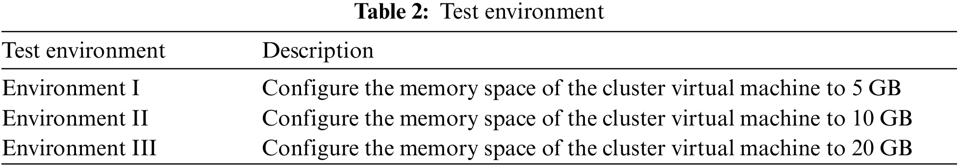
The experiment uses the dynamic and adjustable resource characteristics of Proxmox VE to set up experimental environments with different memory sizes for the nodes in a cluster. The test environment is listed in Table 2.

4.2 Data Sets

The experiments proceed with all jobs with real data sets collected from the web to verify that the proposed approaches can effectively improve business intelligence performance in big data analytics. User inputs the SQL commands related to a certain real data set and measures the job execution time consumed in a specific SQL interface. The real data sets collected from the web includes (1) world-famous books [33], (2) production machine load [34], (3) semiconductor product yield [35], (4) temperature, rainfall, and electricity consumption related to people’s livelihood [36,37], (5) forest flux station data [38], (6) Traffic violations/accidents [39], (7) Analysis of obesity factors [40], (8) Airport flight data [41]. The detailed information about real data sets describes as follows:

(1) World-famous books

This test is first to read the full text of the world-famous books as follows: Alice’s Adventures in Wonderland, The Art of War, Adventures of Huckleberry Finn, Sherlock Holmes, and The Adventures of Tom Sawyer. After that, the word count task counts the number of occurrences of words, and sorts them from high-hit to low-hit in order. An example of plain text file of Alice’s Adventures in Wonderland is shown in Fig. 24.

Figure 24: Plain text file of Alice’s Adventures in Wonderland

(2) Production machine load

Fig. 25 is a product production process report provided by Taiwan’s large packaging and testing factory. The content includes the product number, the responsible employee, the name of the production machine, etc. The file format is .xls format. The purpose is to find the production machines used too frequently or too low in the production schedule and provide the decision-making analysis of the person in charge of the future schedule. Count the number of times the production machine is used and calculate the overall sample standard deviation. According to the concept of normal distribution, find out the data outside the “mean ± 2 * standard deviation” range and treat it as a machine that may be Overloading or Underloading.

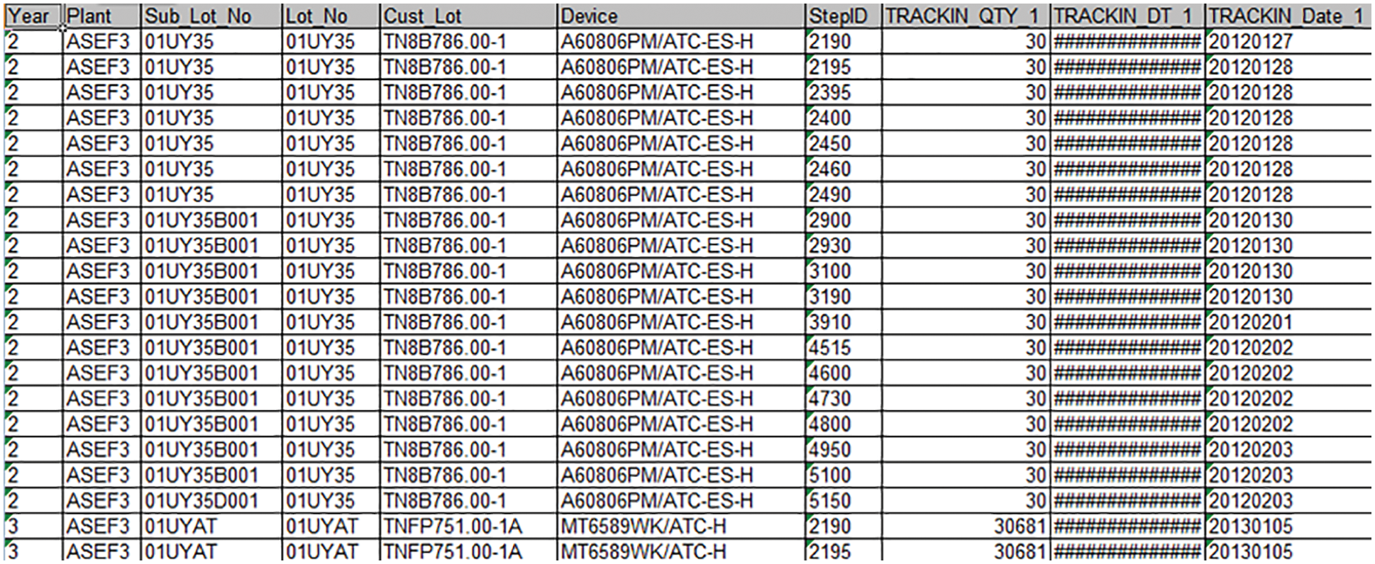
Figure 25: Records of production machine loading

(3) Semiconductor product yield

In Fig. 26, the product test data provided by a significant packaging and testing company in Taiwan includes various semiconductor test items and PASS or FAIL results. The file format is a standard .csv format (separated by commas). The purpose is to calculate the yield rate of the product to see if it meets the company’s yield rate standard (99.7%).

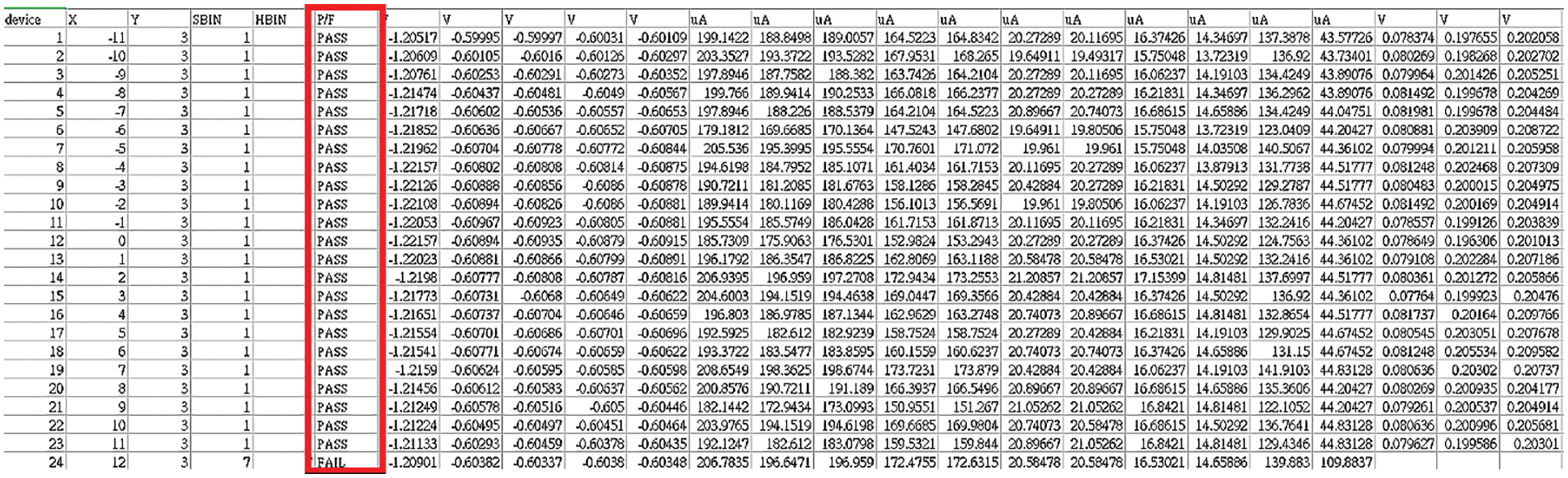
Figure 26: Records of semiconductor product

(4) Temperature, rainfall, and electricity consumption related to livelihood

The website of Taiwan meteorological bureau has collected the rainfall and temperature data, as shown in Fig. 27. The website of TAIPOWER has provided livelihood electricity data, as shown in Fig. 28. For both of them data collection period is from January 01, 2007 to April 30, 2020. The purpose is to find the correlation between rainfall, temperature, and electricity consumption in Taiwan. Based on statistical “Correlation,” the correlation coefficient between the data is calculated and displayed as positive, negative, or no correlation. A certain linear correlation exists when 0 < |r| < 1 between the two variables. The closer |r| approaches to 1, the closer the linear relationship between the two variables is. Contrarily, the closer |r| approaches to 0, the weaker the linear relationship between the two variables is. Generally, it can be divided into three levels: |r| < 0.4 is a low-degree linear correlation; 0.4 ≤ |r| < 0.7 is a significant correlation; 0.7 ≤ |r| < 1 is a high-degree linear correlation.

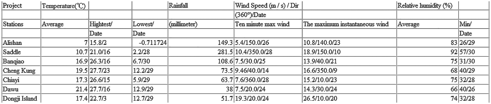
Figure 27: Records of temperature and rainfall

Figure 28: Records of livelihood electricity consumption

(5) Forest flux station data

In Fig. 29, EU Open Data Portal has provided the forest flux station data that contains various flux information, including time and location, illuminance, soil information, and atmospheric flux. The file format is a standard .csv format (separated by commas). The purpose is to calculate the correlation coefficient between the CO2 flux coefficient and the light intensity, temperature, and humidity, respectively, to examine the degree of correlation.

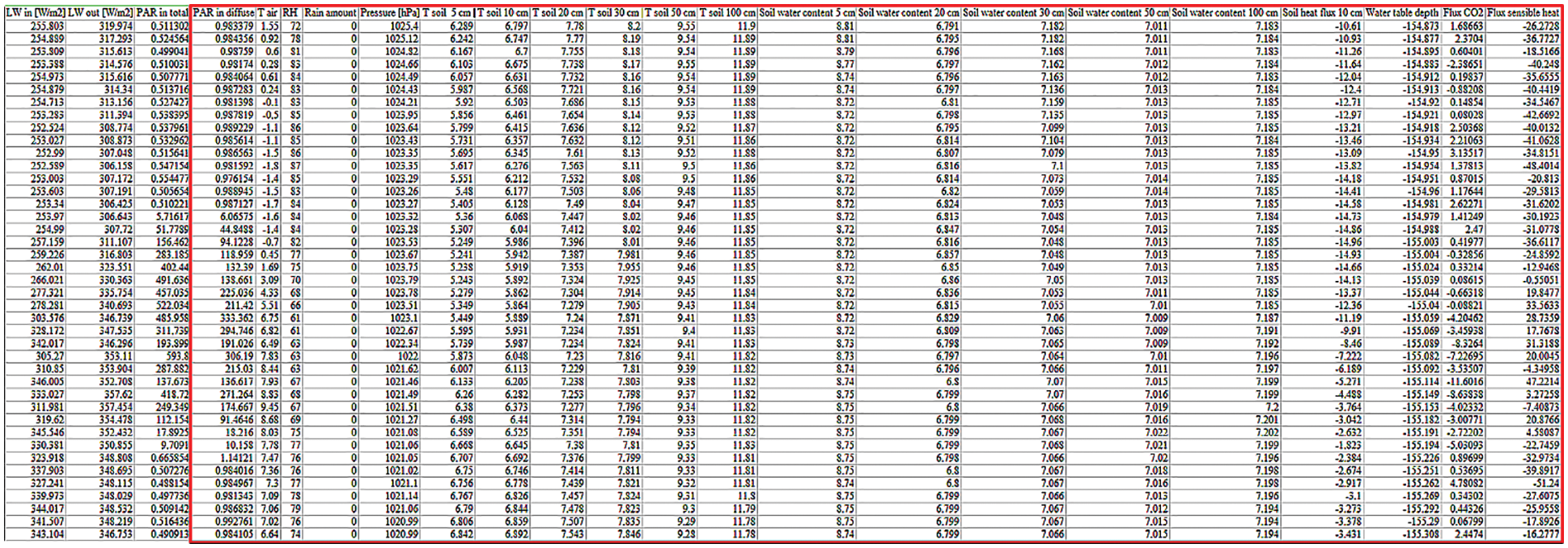
Figure 29: Records of forest flux station

(6) Traffic violations/accidents

Fig. 30 has given the information about traffic violation/accident recorded from Maryland state in USA. Data are in the standard .csv format, i.e., each item separated by commas. Calculate the frequency statistics of monthly traffic violations and accident locations.

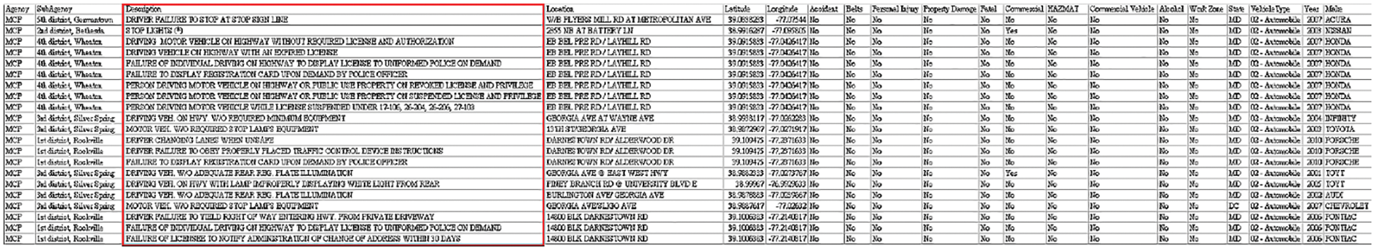
Figure 30: Records of traffic violation/accident

(7) Analysis of obesity factors

U.S. government has published the information about the obesity factors from 2011 to 2019, as shown in Fig. 31. Data are in the standard .csv format, i.e., each item separated by commas. The objective of this test is to analyze the relationship between age, weekly exercise status, vegetable and fruit intake, and BMI through data statistics. Therefore, people can understand whether these factors affect human’s body overweight.

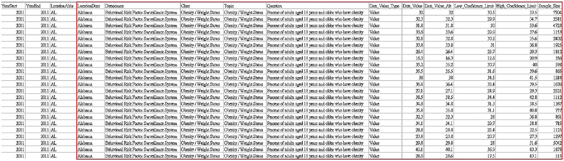
Figure 31: Records of obesity factor

(8) Airport flight data

Fig. 32 has shown the airport flight information recorded from New York airports in USA. Data are in the standard .csv format, i.e., each item separated by commas. This test is to calculate the proportion of the airport’s flights to Taiwan in the total flights in the year.

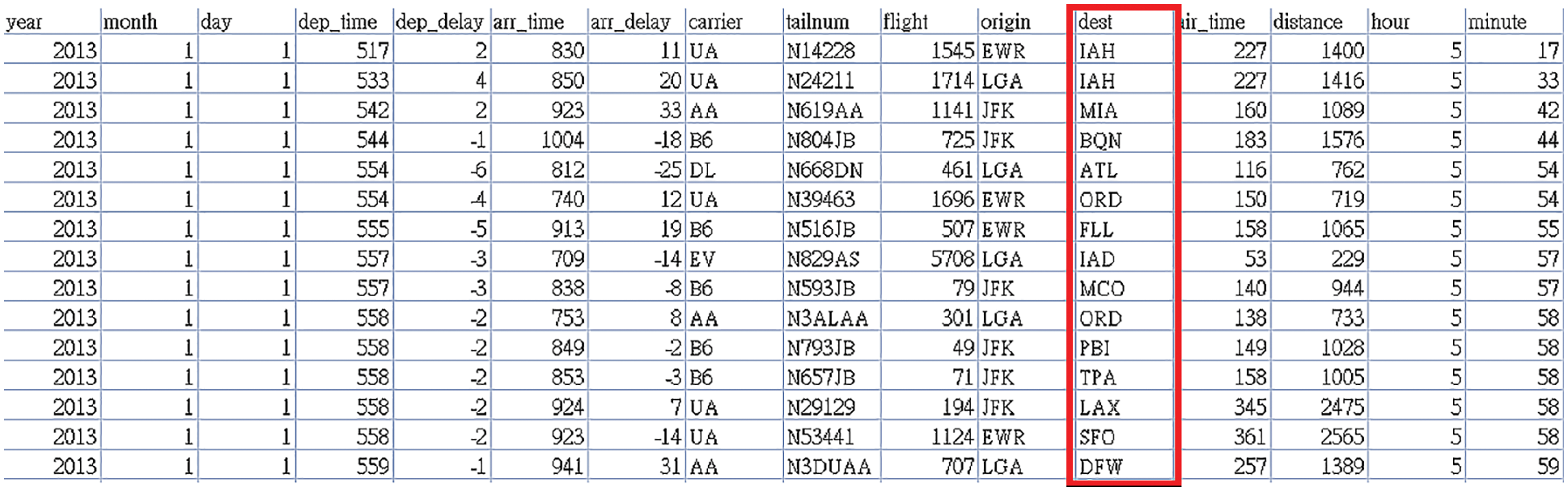
Figure 32: Records of airport flight information

4.3 Data Retrieval Experiment

This experiment tested each data set in different experimental environments, executed them according to the issued SQL commands, and compared their performance using different approaches. Table 3 has listed the different approaches applied in the experiments.

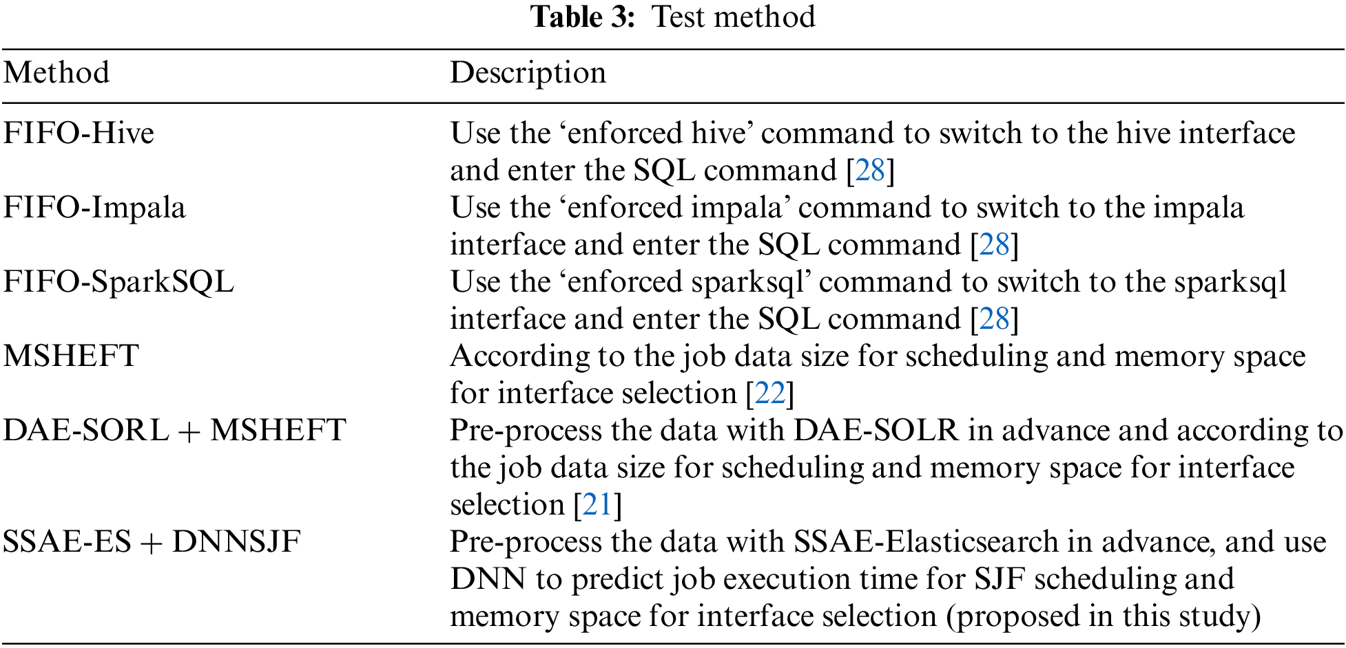
In Table 3, MSHEFT, DAE-SOLR + MSHEFT, and SSAE-ES + DNNSJF are different scheduling algorithms, and thus the order of job execution is scheduled in different sequences. In particular, the Hive interface can only complete the mission when the job has a large amount of data for analysis. However, the Impala or SparkSQL interface could not work successfully because the remaining memory size is insufficient. We noted that the performance of the Impala interface is more prominent when the remaining memory size is moderate. When the remaining memory size is significantly large, the SparkSQL interface can perform best due to its in-memory computing capability.

With automatic interface selection, the system can select the appropriate SQL interface and accept the SQL command from a user to perform the corresponding job in different scheduling algorithms, MSHEFT, DAE-SOLR + MSHEFT, and SSAE-ES + DNNSJF. If the data set sored in HDFS has completed data retrieval optimization in advance, the optimized data clustering and indexing can significantly reduce the average execution time of data searching. Experimental results have shown each job execution time, as shown in Figs. 33–35, and the average job execution time and system throughput, as listed in Tables 4–6.

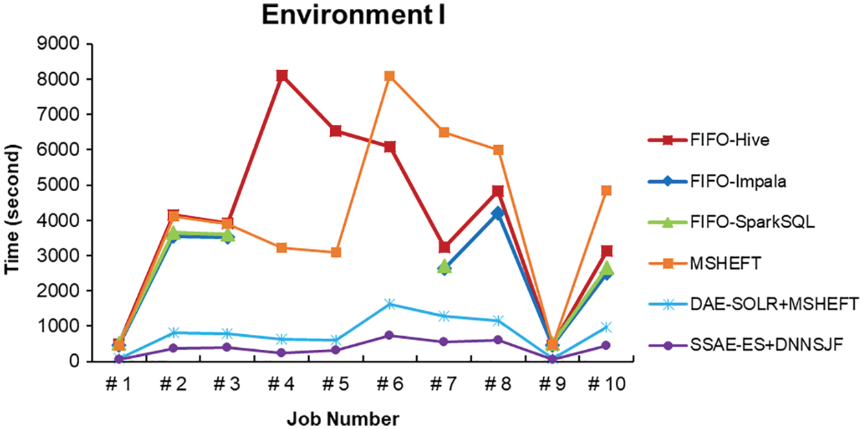
Figure 33: Job execution time of various methods in Environment I

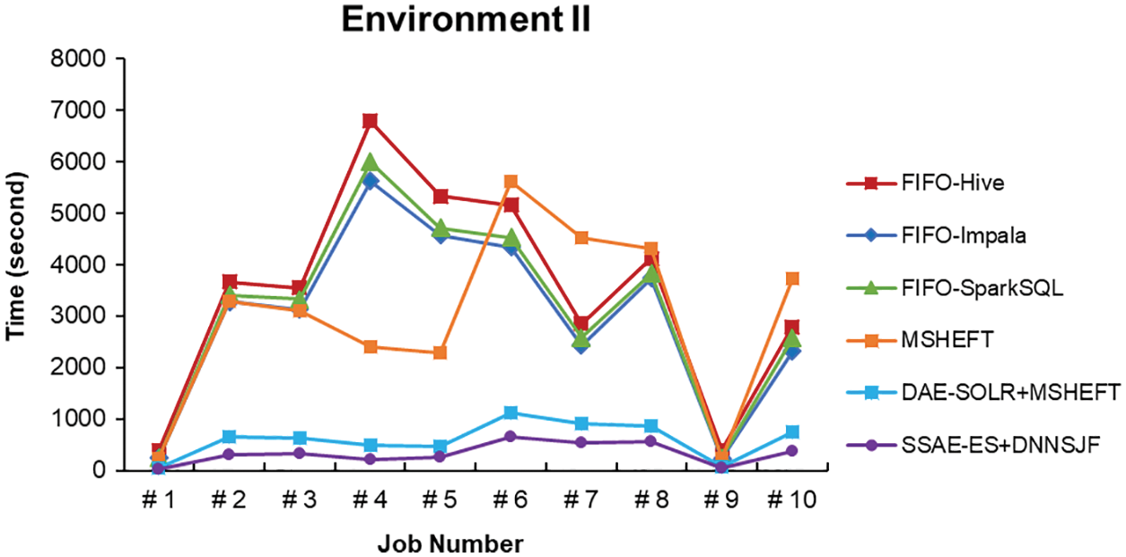
Figure 34: Job execution time of various methods in Environment II

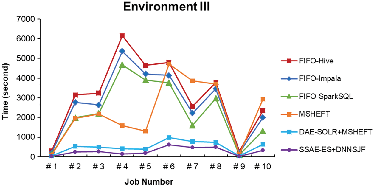
Figure 35: Job execution time of various methods in Environment III

4.4 Job Scheduling Experiment

Since this study uses an automatic SQL interface selection, the appropriate SQL interface can be automatically selected to perform data analysis according to available memory size. Therefore, the experiments use this way to test an appropriate SQL interface selected to perform data analysis in different environments and compares the average job waiting time for execution among different scheduling algorithms.

To comply with the requirement of the experimental tests hereafter, they will use SSAE and Elasticsearch for all data sets to execute data retrieval together with the various job scheduling, as listed in Table 7. We here tested the experimental environment I, II, and III, as listed in Table 2. Since FIFO, MSHEFT, and DNNSJF are different job scheduling algorithms, the job scheduling algorithms will execute in a different order.

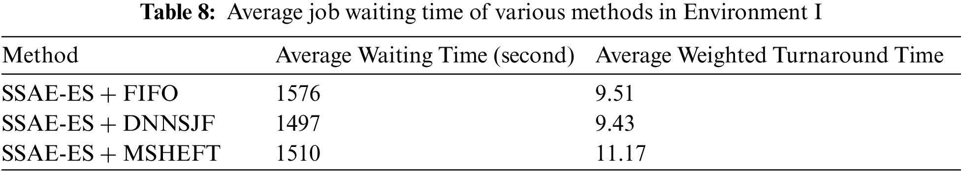
According to the experimental results, different data analysis jobs take different times. Generally speaking, the job scheduling performance of MSHEFT is good. However, the MSHEFT algorithm will do the same job scheduling as the FIFO algorithm when different jobs have the same data set size. The experimental results show that the proposed approach DNNSJF algorithm obtains the shortest average waiting time and average weighted turnaround time for each job execution, followed by the MSHEFT scheduling algorithm that schedules the jobs based on the amount of data size, and the FIFO algorithm reaches the poor one. The experimental results have shown the waiting time for each job execution, as shown in Figs. 36–38. They have also shown the average job waiting time for execution and average weighted turnaround time, as listed in Tables 8–10.

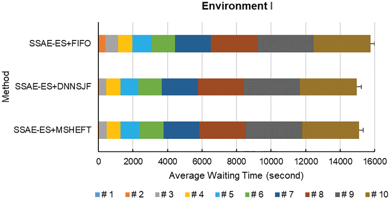
Figure 36: Job waiting time of various methods in Environment I

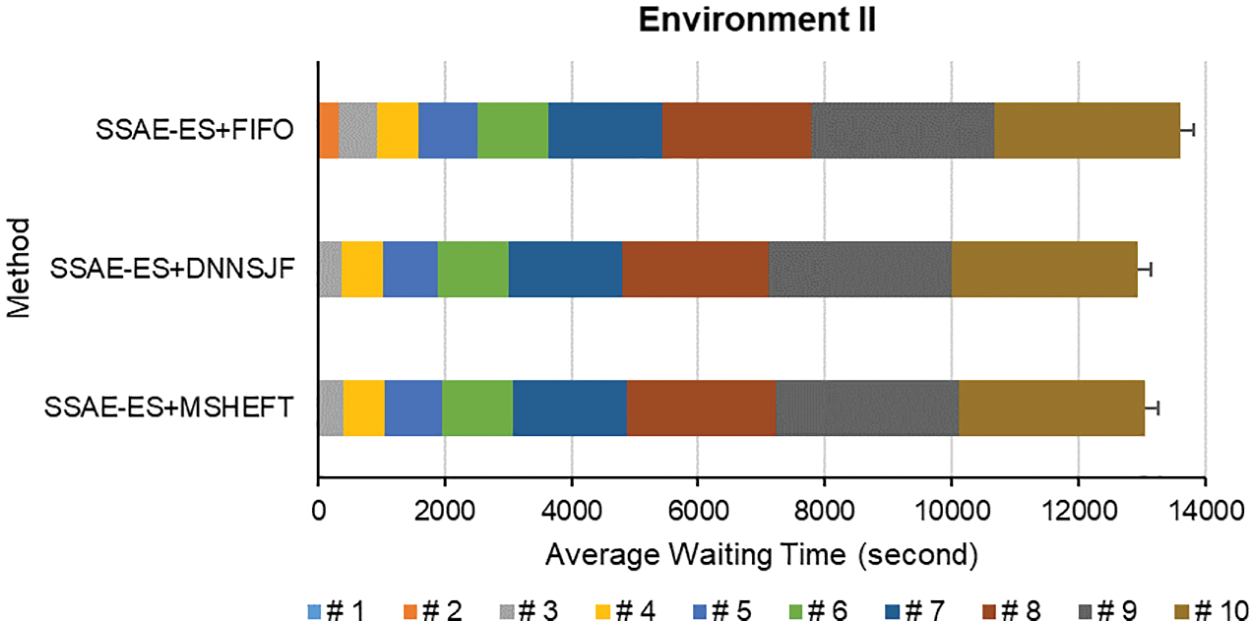
Figure 37: Job waiting time of various methods in Environment II

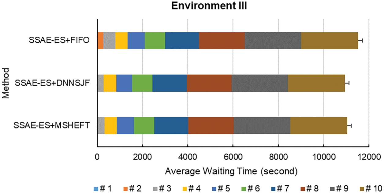
Figure 38: Job waiting time of various methods in Environment III

4.5 Hypothesis Testing

The data tested in this study cannot be directly assumed to obey a specific distribution, and this study should test it using a nonparametric statistical method. This paper will introduce the Wilcoxon signed-rank test [42] as a hypothesis testing in this study, which is a nonparametric statistical method for testing a single sample. In Table 11, the first hypothesis testing will proceed with the Wilcoxon signed-rank test between the previous method DAE-SOLR + MSHEFT and the proposed approach SSAE-ES + DNNSJF where test has sampled 30 valid data from Experiments I, II, and III of data retrieval. Next, the second one will proceed with the Wilcoxon signed-rank test between the previous method SSAE-ES + MSHEFT and the proposed approach SSAE-ES + DNNSJF where the test has sampled nine valid data from Experiments I, II, and III of job scheduling.

Assuming a one-tailed test of α = 0.05, the null hypothesis and the alternative hypothesis are as follows:

H0:MP=MCHa:MP>MC(4)

In Eq. (4), MP and MC are the median time-consuming of using the previous method and the proposed approach. Assuming that T is the smallest of the positive and negative sorted sums, Eq. (5) expresses the following formula:

T=min{|sumofpositivesequence|,|sumofnegativesequence|}(5)

E(T) in Eq. (6) is the expected value of the random variable T and VAR(T) in Eq. (7) the variance

E(T)=(1+2+…+n)=n(n+1)/4(6)

VAR(T)=12(12+22+…+n2)=n(n+1)(2n+1)/24(7)

When the number of samples is proper (n ≥ 20), Z stands for the test statistic in Eq. (8). If the number of samples is too small (n < 20), Z∗ represents the continuity correction of the test statistic Z in Eq. (9).

Z=|T−E(T)|/|T−E(T)|VAR(T)VAR(T)(8)

Z∗=|T−E(T)|−12/|T−E(T)|−12VAR(T)VAR(T)(9)

As a result, looking-up Z table, the Z value of α = 0.05 is 1.65 that is less than both 4.78 (Z value) and 2.61 (Z∗ value) as shown in Table 11. The decision can reject the null hypothesis H0. That indicates that the sampling data have obtained significant results in the Wilcoxon signed-rank test for the proposed approaches in this paper.

4.6 Discussion

According to the data retrieval experiments, the SSAE-ES approach partitions the vast data to eight data zones successfully, adds sparse constraints to enhance searching capability, and implements an indexing function for the large-scale database to realize fast indexing of target data. Compared with the previous method DAE-SOLR, the SSAE-ES approach effectively improves the speed of data retrieval up to 44∼53% and increases system throughput by 44∼53%. As a result, the proposed approach SSAE-ES outperforms the other alternatives in data retrieval in the experiments. The results of the experiments showed the strengths of the proposed SSAE-ES algorithm. Besides, a statistical test using Wilcoxon signed-rank test can support the claim on improved results obtained with the proposed approach. SparkSQL performs better data retrieval than Impala or Hive in the experiments given considerable memory size.

Next, according to the job scheduling experiments, the MSHEFT algorithm performs job scheduling based on the data size for each job. It can decrease the waiting time of job execution in a queue. However, when it comes up with different jobs with the same data size, the MSHEFT algorithm proceeds with the job scheduling just like a FIFO scheduling. That is a bad situation. Therefore, the proposed DNNSJF approach can effectively overcome this problem because it can infer the different execution times for the same data size of many different jobs. Compared with FIFO and MSHEFT job scheduling algorithms, the DNNSJF approach can shorten the job’s average waiting time to 3∼5% and 1∼3%, and the average weighted turnaround time by 0.8%∼09.9% and 16%∼19%. The results of the experiments showed the strengths of the proposed DNNSJF approach. Besides, a statistical test using Wilcoxon signed-rank test can present the claim confirmed on the significance test results with the proposed approach.

The experiments found that in-memory cache will lose part of retrieval data when a block of data size is more extensive than 100,000 bytes. Memcached may cause data loss when it has written a large amount of retrieval data back to the in-memory cache in a single stroke. The experiments showed the weaknesses of the Memcached used in the in-memory cache.

5  Conclusion

In this paper, the theoretical implication is to improve the efficiency of big data analytics on two aspects: speed up data retrieval in big data analytics, increase system throughput concurrently, and optimize job scheduling to shorten the waiting time for job execution in a queue. There are two significant findings in this study. First, this study explores the advanced searching and indexing approaches to improve the speed of data retrieval up to 53% and increase system throughput by 53% compared with the previous method. Next, this study exploits the deep learning model to predict the job execution time used to arrange prioritized job scheduling, shortening the average waiting time up to 5% and the average weighted turnaround time by 19%. As a result, big data analytics and its application of business intelligence can achieve high performance and high efficiency based on our proposed approaches in this study. However, the system has shortcomings about the limits of in-memory cache operations. When a large amount of data in a single in-memory cache block (more than 100,000 bytes) occurs, we will lose part of the block and not write the retrieval results entirely into the in-memory cache. Moreover, the system can only write a single stroke to the in-memory cache sequentially, i.e., time-consuming. We have to find a way to improve both problems as mentioned earlier in the future.

According to the themes discussed in this paper, there are some aspects worth exploring more profoundly in the future. The first is to find a model with better precision in the job execution time prediction. Looking for the other deep learning model, e.g., a long short-term memory is technically feasible instead of the DNN model. Secondly, you can write a JDBC interface to connect with the main program to extend the other SQL interfaces. Finally, we have to find a better solution to the limits of in-memory cache operations about the size of a block and a single sequential stroke writing to avoid losing part of blocks while writing.

Author Contributions: B.R.C. and Y.C.L. conceived and designed the experiments; H.F.T. collected the experimental dataset, and H.F.T. proofread the paper; B.R.C. wrote the paper.

Funding Statement: This paper is supported and granted by the Ministry of Science and Technology, Taiwan (MOST 110-2622-E-390-001 and MOST 109-2622-E-390-002-CC3).

Conflicts of Interest: The authors declare that there is no conflict of interests regarding the publication of the paper.

References

1. Guedea-Noriega, H. H., García-Sánchez, F. (2019). Semantic (Big) Data analysis: An extensive literature review. IEEE Latin America Transactions, 17, 796–806. DOI 10.1109/TLA.2019.8891948. [Google Scholar] [CrossRef]
2. Gheorghe, A. G., Crecana, C. C., Negru, C., Pop, F., Dobre, C. (2019). Decentralized storage system for edge computing decentralized storage system for edge computing. 2019 18th International Symposium on Parallel and Distributed Computing (ISPDC), Amsterdam, Netherlands. DOI 10.1109/ISPDC.2019.00009. [Google Scholar] [CrossRef]
3. Lee, J., Kim, B., Chung, J. M. (2019). Time estimation and resource minimization scheme for apache spark and hadoop Big Data systems with failures. IEEE Access, 7, 9658–9666. DOI 10.1109/ACCESS.2019.2891001. [Google Scholar] [CrossRef]
4. Deshpande, P. M., Margoor, A., Venkatesh, R. (2018). Automatic tuning of SQL-on-Hadoop engines on cloud platforms. 2018 IEEE 11th International Conference on Cloud Computing (CLOUD), San Francisco, CA, USA. DOI 10.1109/CLOUD.2018.00071. [Google Scholar] [CrossRef]
5. Hadjar, K., Jedidi, A. (2019). A new approach for scheduling tasks and/or jobs in Big Data Cluster. 2019 4th MEC International Conference on Big Data and Smart City (ICBDSC), Muscat, Oman. [Google Scholar]
6. Sun, H., Liu, Z., Wang, G., Lian, W., Ma, J. (2019). Intelligent analysis of medical Big Data based on deep learning. IEEE Access, 7, 142022–142037. DOI 10.1109/ICBDSC.2019.8645613. [Google Scholar] [CrossRef]
7. Wang, F. Y., Zhang, J. J., Zheng, X., Wang, X., Yuan, Y. et al. (2016). Where does AlphaGo go: From church-turing thesis to AlphaGo thesis and beyond. IEEE/CAA Journal of Automatica Sinica, 3, 113–120. DOI 10.1109/JAS.2016.7471613. [Google Scholar] [CrossRef]
8. Lu, M., Li, F. (2020). Survey on lie group machine learning. Big Data Mining and Analytics, 3, 235–258. DOI 10.26599/BDMA.2020.9020011. [Google Scholar] [CrossRef]
9. Klinefelter, E., Nanzer, J. A. (2020). Interferometric microwave radar with a feedforward neural network for vehicle speed-over-ground estimation. IEEE Microwave and Wireless Components Letters, 30, 304–307. DOI 10.1109/LMWC.2020.2966191. [Google Scholar] [CrossRef]
10. Ma, L., Bao, W., Yuan, W., Huang, T., Zhao, X. (2017). A Mongolian information retrieval system based on solr. 2017 9th International Conference on Measuring Technology and Mechatronics Automation (ICMTMA), Changsha, China. DOI 10.1109/ICMTMA.2017.0087. [Google Scholar] [CrossRef]
11. Yan, B., Han, G. (2018). Effective feature extraction via stacked sparse autoencoder to improve intrusion detection system. IEEE Access, 6, 41238–41248. DOI 10.1109/ACCESS.2018.2858277. [Google Scholar] [CrossRef]
12. Chen, D., Chen, Y., Brownlow, B. N., Kanjamala, P. P., Garcia Arredondo, C. A. et al. (2016). Real-time or near real-time persisting daily healthcare data into HDFS and ElasticSearch index inside a Big Data platform. IEEE Transactions on Industrial Informatics, 13, 595–606. DOI 10.1109/TII.2016.2645606. [Google Scholar] [CrossRef]
13. Chen, B., Liu, Y., Zhang, C., Wang, Z. (2018). Time series data for equipment reliability analysis with deep learning. IEEE Access, 8, 105484–105493. DOI 10.1109/ACCESS.2020.3000006. [Google Scholar] [CrossRef]
14. Teraiya, J., Shah, A. (2018). Comparative study of LST and SJF scheduling algorithm in soft real-time system with its implementation and analysis. 2018 International Conference on Advances in Computing, Communications and Informatics (ICACCI), Bangalore, India. DOI 10.1109/ICACCI.2018.8554483. [Google Scholar] [CrossRef]
15. Guo, W., Tian, W., Ye, Y., Xu, L., Wu, K. (2020). Cloud resource scheduling with deep reinforcement learning and imitation learning. IEEE Internet of Things Journal, 8(5), 3576–3586. DOI 10.1109/JIOT.2020.3025015. [Google Scholar] [CrossRef]
16. Yeh, T., Huang, H. (2018). Realizing prioritized scheduling service in the hadoop system. 2018 IEEE 6th International Conference on Future Internet of Things and Cloud (FiCloud), Barcelona, Spain. DOI 10.1109/FiCloud.2018.00015. [Google Scholar] [CrossRef]
17. Thangaselvi, R., Ananthbabu, S., Jagadeesh, S., Aruna, R. (2015). Improving the efficiency of MapReduce scheduling algorithm in hadoop. 2015 International Conference on Applied and Theoretical Computing and Communication Technology (iCATccT), Davangere, India. DOI 10.1109/ICATCCT.2015.7456856. [Google Scholar] [CrossRef]
18. Sinaga, K. P., Yang, M. S. (2020). Unsupervised K-means clustering algorithm. IEEE Access, 8, 80716–80727. DOI 10.1109/ACCESS.2020.2988796. [Google Scholar] [CrossRef]
19. Marquez, E. S., Hare, J. S., Niranjan, M. (2018). Deep cascade learning. IEEE Transactions on Neural Networks and Learning Systems, 29, 5475–5485. DOI 10.1109/TNNLS.2018.2805098. [Google Scholar] [CrossRef]
20. Gupta, A., Thakur, H. K., Shrivastava, R., Kumar, P., Nag, S. (2017). A big data analysis framework using apache spark and deep learning. 2017 IEEE International Conference on Data Mining Workshops (ICDMW), New Orleans, LA, USA. DOI 10.1109/ICDMW.2017.9. [Google Scholar] [CrossRef]
21. Lee, Y. D., Chang, B. R. (2018). Deep learning-based integration and optimization of rapid data retrieval in Big Data platforms (Master Thesis), Department of Computer Science and Information Engineering, National University of Kaohsiung, Taiwan. DOI 10.1155/2021/9022558. [Google Scholar] [CrossRef]
22. Chang, B. R., Lee, Y. D., Liao, P. H. (2017). Development of multiple Big Data analytics platforms with rapid response. Scientific Programming, 2017, 6972461. DOI 10.1155/2017/6972461. [Google Scholar] [CrossRef]
23. Abualigah, L., Yousri, D., Abd Elaziz, M., Ewees, A. A., Al-Qaness, M. A. et al. (2021). Aquila optimizer: A novel meta-heuristic optimization algorithm. Computers & Industrial Engineering, 157, 107250. DOI 10.1016/j.cie.2021.107250. [Google Scholar] [CrossRef]
24. Abualigah, L., Abd Elaziz, M., Sumari, P., Geem, Z. W., Gandomi, A. H. (2022). Reptile search algorithm (RSAA nature-inspired meta-heuristic optimizer. Expert Systems with Applications, 191, 116158. DOI 10.1016/j.eswa.2021.116158. [Google Scholar] [CrossRef]
25. Abualigah, L., Diabat, A., Sumari, P., Gandomi, A. H. (2021). Applications, deployments, and integration of Internet of Drones (IoDA review. IEEE Sensors Journal, 21(22), 25532–25546. DOI 10.1109/JSEN.2021.3114266. [Google Scholar] [CrossRef]
26. Liu, J., Li, C., Yang, W. (2018). Supervised learning via unsupervised sparse autoencoder. IEEE Access, 6, 73802–73814. DOI 10.1109/ACCESS.2018.2884697. [Google Scholar] [CrossRef]
27. Karacan, L., Erdem, A., Erdem, E. (2017). Alpha matting with KL-divergence-based sparse sampling. IEEE Transactions on Image Processing, 26, 4523–4536. DOI 10.1109/TIP.2017.2718664. [Google Scholar] [CrossRef]
28. Chang, B. R., Tsai, H. F., Lee, Y. D. (2018). Integrated high-performance platform for fast query response in Big Data with hive, impala, and SparkSQL: A performance evaluation. Applied Sciences, 8(9), 1514, 26. DOI 10.3390/app8091514. [Google Scholar] [CrossRef]
29. Topcuoglu, H., Hariri, S., Wu, M. (2002). Performance-effective and low-complexity task scheduling for heterogeneous computing. IEEE Transactions on Parallel and Distributed Systems, 13(3), 260–274. DOI 10.1109/71.993206. [Google Scholar] [CrossRef]
30. Carra, D., Michiardi, P. (2016). Memory partitioning and management in memcached. IEEE Transactions on Services Computing, 12, 564–576. DOI 10.1109/TSC.2016.2613048. [Google Scholar] [CrossRef]
31. Ali, A. M., Farhan, A. K. (2020). A novel improvement with an effective expansion to enhance the MD5 hash function for verification of a secure e-document. IEEE Access, 8, 80290–80304. DOI 10.1109/ACCESS.2020.2989050. [Google Scholar] [CrossRef]
32. Verma, C., Stoffová, V., Illés, Z., Tanwar, S., Kumar, N. (2020). Machine learning-based student’s native place identification for real-time. IEEE Access, 8, 130840–130854. DOI 10.1109/ACCESS.2020.3008830. [Google Scholar] [CrossRef]
33. Lin, Y. C. (2021). World-famous books. https://github.com/did56789/World-famous-books.git. [Google Scholar]
34. Lin, Y. C. (2021). Production machine load data. https://github.com/did56789/Production-machine-load.git. [Google Scholar]
35. Lin, Y. C. (2021). Semiconductor product yield data. https://github.com/did56789/Semiconductor-product-yield.git. [Google Scholar]
36. MOTC, Central Weather Bureau (2021). Rainfall and temperature data. https://www.cwb.gov.tw/V8/C/C/Statistics/monthlydata.html. [Google Scholar]
37. Taiwan Power Company (2021). Livelihood electricity data. https://www.taipower.com.tw/tc/page.aspx?mid=5554. [Google Scholar]
38. EU Open Data Portal (2021). The forest flux station data. https://data.europa.eu/data/datasets/jrc-abcis-it-sr2-2017?locale=en. [Google Scholar]
39. Lin, Y. C. (2021). Traffic violations accidents data. https://github.com/did56789/Traffic-violations-accidents.git. [Google Scholar]
40. Centers for Disease Control and Prevention (2021). Nutrition, physical activity, and obesity-behavioral risk factor surveillance system. https://chronicdata.cdc.gov/Nutrition-Physical-Activity-and-Obesity/Nutrition-Physical-Activity-and-Obesity-Behavioral/hn4x-zwk7. [Google Scholar]
41. Lin, Y. C. (2021). Airport flight data. https://github.com/did56789/Airport-flight-data.git. [Google Scholar]
42. Zhang, Z., Hong, W. C. (2021). Application of variational mode decomposition and chaotic grey wolf optimizer with support vector regression for forecasting electric loads. Knowledge-Based Systems, 228, 107297. DOI 10.1016/j.knosys.2021.107297. [Google Scholar] [CrossRef]
Cite This Article
Copyright © 2023 The Author(s). Published by Tech Science Press.
This work is licensed under a Creative Commons Attribution 4.0 International License , which permits unrestricted use, distribution, and reproduction in any medium, provided the original work is properly cited.
Downloads
Citation Tools