
 Submit a Paper
 Propose a Special lssue
 Open Access
ARTICLE
Improved High Order Model-Free Adaptive Iterative Learning Control with Disturbance Compensation and Enhanced Convergence
Key Laboratory of Advanced Process Control for Light Industry (Ministry of Education), Institute of Automation, Jiangnan University, Wuxi, 214122, China
* Corresponding Author: Zhiguo Wang. Email:
(This article belongs to the Special Issue: Advances on Modeling and State Estimation for Industrial Processes)
Computer Modeling in Engineering & Sciences 2023, 134(1), 343-355. https://doi.org/10.32604/cmes.2022.020569
Received 01 December 2021; Accepted 22 February 2022; Issue published 24 August 2022
 View Full Text
 Download PDF
Abstract
In this paper, an improved high-order model-free adaptive iterative control (IHOMFAILC) method for a class of nonlinear discrete-time systems is proposed based on the compact format dynamic linearization method. This method adds the differential of tracking error in the criteria function to compensate for the effect of the random disturbance. Meanwhile, a high-order estimation algorithm is used to estimate the value of pseudo partial derivative (PPD), that is, the current value of PPD is updated by that of previous iterations. Thus the rapid convergence of the maximum tracking error is not limited by the initial value of PPD. The convergence of the maximum tracking error is deduced in detail. This method can track the desired output with enhanced convergence and improved tracking performance. Two examples are used to verify the convergence and effectiveness of the proposed method.Keywords
Generally, there are two strategies for controller design. One is based on the exact process information, and the other is based on the input-output data which is a model-free controller design strategy. Many practical industrial processes contain nonlinearity, uncertainty, and time-varying characteristics. In this case, model-based control becomes inapplicable because it is difficult to obtain an accurate mathematical model of the controlled object. In recent years, the model-free methods have attracted the attention of many researchers because of their remarkable advantages and have achieved some valuable results [1,2].
Model-free adaptive control (MFAC) is one of the typical data-driven control methods proposed by Hou [3]. The principle of the MFAC algorithm is to continuously generate a dynamic linearization model containing pseudo partial derivative (PPD), which transforms the nonlinear system into a time-varying linearized model that utilizes the input and output data of every step [4]. Compared with the model-based algorithm, model-free adaptive control has the characteristics of fewer identification parameters and fewer calculations. This method has been applied in various fields, for example, process control [5], motor system [6], and so on. Arimoto et al. [7] proposed iterative learning control (ILC), which is suitable for a class of controlled objects with repetitive running characteristics, such as robots with reciprocating operation characteristics [8] and a chemical reactor in a batch process [9]. Iterative learning control was applied to improve the tracking performance of nonlinear processes whose model and parameters are unknown [10]. Zhao et al. [11] used iterative learning to design the unbiased finite impulse response. Combining the advantages of model-free adaptive control with iterative learning control, model-free adaptive iterative learning control (MFAILC) was proposed in [12]. Unlike the iterative learning control with fixed learning gain, the learning gain of model-free adaptive iterative learning control is time-varying. It transforms the original nonlinear time-domain into a nonlinear iterative domain and can be applied to other nonlinear controlled objects whose structures and parameters are time-varying [13,14]. Thus MFAILC algorithm has better stability and adaptability for complex systems [15].
Based on the previous research results, many researchers have further investigated the model-free adaptive iterative learning control algorithm. In [16], an improved model-free adaptive iterative learning control method which based on an encoding and decoding quantization mechanism was proposed for a class of unknown nonlinear systems with data quantization. Li [17] adopted a neural network to optimize the control law and the penalty of PPD. For a class of nonlinear discrete systems with load disturbance and data loss, Hua et al. [18] proposed a control method with data compensation. Model-free adaptive iterative learning control was applied to a multi-agent system by Bu et al. [19]. Chi et al. [20] proposed a high order model-free adaptive iterative learning control, which uses the input and output information of the previous iterations to construct a new control input. It is obvious from the above observations that MFAILC has made great progress in theoretical research. In the control process, convergence is a critical index for ILC so as to MFAILC [21]. However, the convergence speed is related to the initial pseudo partial derivative, and it often takes several experiments to get the appropriate value of the initial PPD [22]. The slower convergence will deteriorate the performance of the controlled process [23].
To obtain a faster convergence, the high-order algorithm was used to estimate the value of pseudo partial derivatives, which introduced more parameters to be adjusted unexpectedly [24]. This method brings more difficulties in tuning parameters. On the basis of the former, this paper proposed an improved high-order model-free adaptive iterative control (IHOMFAILC). The main contributions of this paper are as follows:
• An improved PPD estimation algorithm, which takes the average value of the previous PPDs can achieve faster convergence without introducing more parameters.
• A differential module is introduced into the criteria function of the controller to compensate for the dynamic performance of the system under random disturbance.
• The proposed method contains fewer parameters to design and with the number of iterations increases, the maximum error gradually converges to zero.
The rest of this paper is organized as follows: Section 2 introduces the basic principle of model-free adaptive iterative learning control. The proposed method with disturbance compensation and enhanced convergence is shown in detail in Section 3. In Section 4, the convergence and stability of the proposed algorithm are proved in detail. Two examples are used to illustrate the effectiveness of the method in Section 5 and the conclusions are drawn in Section 6.
Consider the following nonlinear discrete-time SISO system:
where
The following two assumptions are given for system (1) to make the discussion rigorous:
Assumption 1: The partial derivative of the nonlinear function
Assumption 2: System (1) satisfies the generalized Lipschitz condition, that is, for any time
where
Lemma 1: For any nonlinear system that satisfies assumptions 1 and 2, if
where
In order to design the control law, the following criteria function is considered:
where
Substituting (3) into (4) and minimizing (4) with respect to
where
As with solving
where
Taking the derivative of Eq. (4) with respect to
where
In order to make the algorithm estimate value of Eq. (7) more accurate, the following reset algorithm is denoted: if
where
However, the rapidity of convergence of the maximum error of MFAILC is related to the value of the initial PPD. The larger the value is, the slower the convergence rate is and the larger the error is. Therefore, an improved method is proposed to solve the above problem.
3 Improved High-Order Model-Free Adaptive Iterative Learning Control Method
In the proposed method, a differential link is added to compensate for the impact of random disturbance on the system and only use input and output data to design the control law.
Consider the following criteria function:
where
To get the optional solution, we minimizing (10) with respect to
according to (11),
Unlike other high-order algorithms designed based on control input [25] and tracking error terms [26], the improved high-order algorithm uses previous iterations to estimate the PPD. Compared to the algorithm in [24], the improved algorithm does not need to take different weight coefficients for the previous PPDs.
If the number of iterations is less than the iteration learning
when the number of iterations is larger than the iteration learning
Taking the partial derivative of
Minimizing Eq. (14) by solving
where
In this section, the convergence of the proposed method is mainly proved. In order to make the following discussion more rigorous, the following assumption is given:
Assumption 3: For all
Assumption 3 is similar to a restriction on the direction of control input gain.
Lemma 2: If system (1) satisfies assumption 1–3, there must exist
1. For all
2. When
3. The close-loop system is BIBO stability, for all
Proof: The first step is to prove that
when
In other cases, when
Subtracting
Denote
When
From Lemma 1 we get
where
when
Substituting Eq. (3) into (24) and taking absolute worthwhile at both sides, we have:
Eq. (25) can finally be simplified as follows:
From Lemma 1, we know
Then the convergence of tracking error and the bounded control input are proved as follows:
Denote if
Since
From Eqs. (28) and (29) we get:
Since
According to Eqs. (28)–(31), we have:
From Eq. (33) we can get, if
Let
Then Eq. (35) can be described as follows:
Let
Let
where
where
According to Eq. (31):
Substituting Eq. (40) into
Eq. (41)
Substituting (42) into (39) yields:
When
Thus the following inequality is given:
Substituting
According to inequality (38) and (46), with the increase of the number of iterations
From inequality (33), we have:
Eq. (47) can be reorganized as follows:
This implies that
Example 1: Consider the following time-varying system [14]:
The desired output is:
where
Table 1 shows the ITAE performance index of the two methods. When the number of iterations is set to 10, 20, 30, and 40 while other parameters are unchanged, the IATE values of IHOMFAILC is less than that of MFAILC. As the number of iterations increase, the IATE values of both methods shows a downward trend. Therefore the proposed method performance index is better.

Fig. 1 shows the tracking results of IHOMFAILC and MFAILC with different iterations. From the 15th iteration result, the proposed method can gradually approach desired output ultimately tracks it at 40 iterations. The output of the MFAILC method at the 40th iteration still has a large error with the expected output.
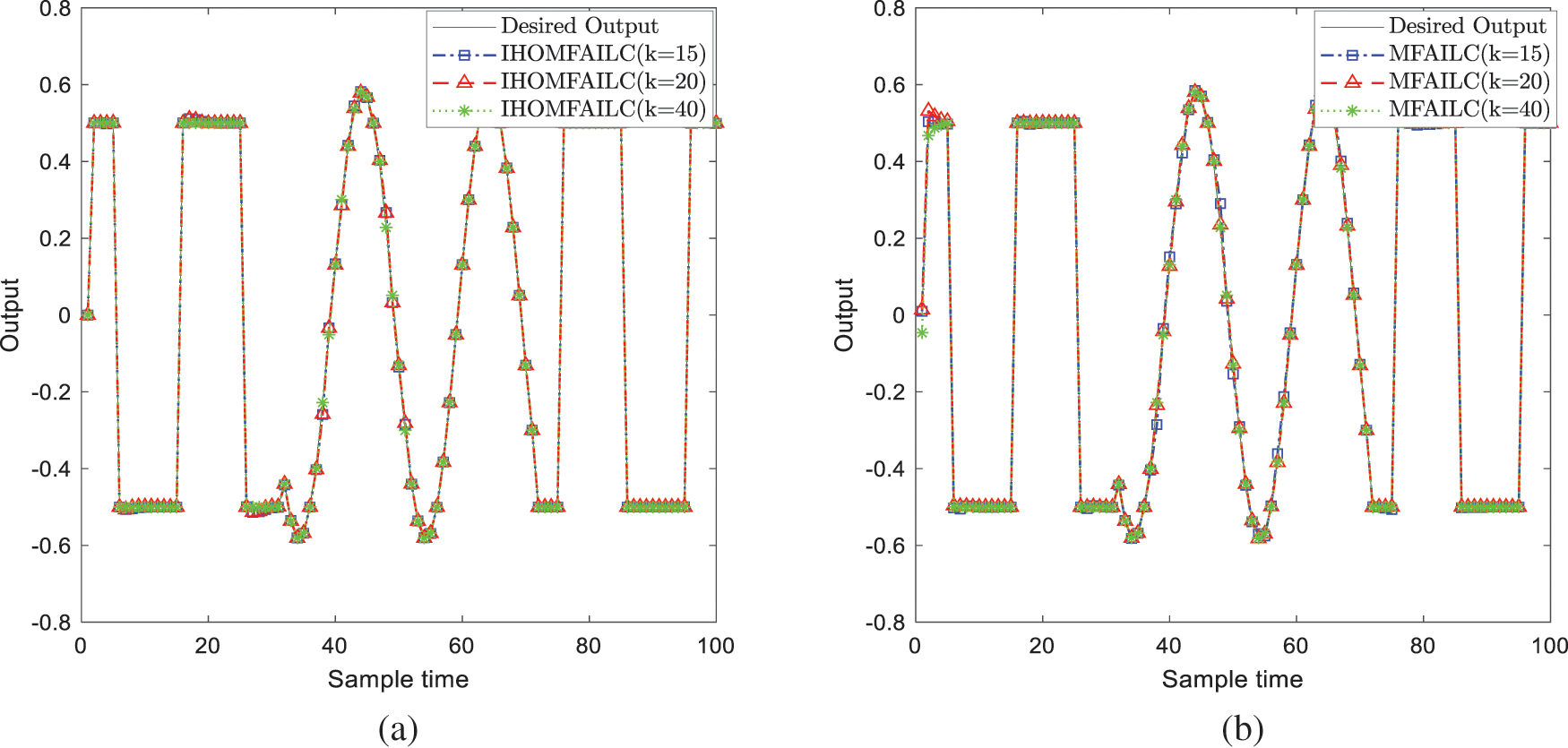
Figure 1: Tracking results of IHOMFAILC and MFAILC with different iterations
The maximum tracking error of IHOMFAILC and MFAILC with different initial PPDs is shown in Fig. 2. As the picture shows, the change of the initial value of PPD has a great impact on the error convergence speed of MFAILC. The proposed method ensures fast convergence and the final error convergence to 0. Results demonstrate that IHOMFAILC can achieve fast convergence with a few attempts to select the best initial value of PPD.
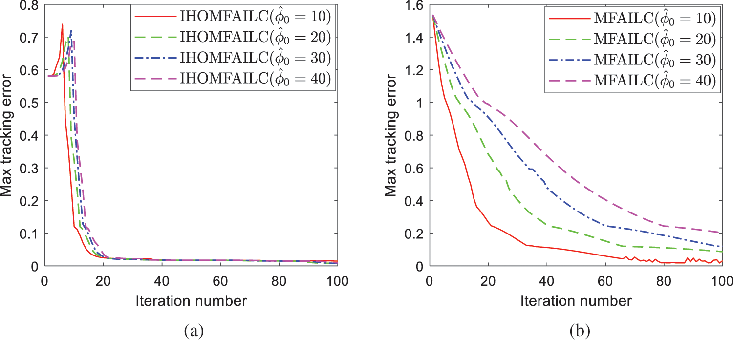
Figure 2: Comparison of max tracking error of MFAILC and IHOMFAILC with different initial PPDs
Example 2: In order to verify the effectiveness of the proposed algorithm, simulation is performed on a permanent magnet DC linear motor [1]. The dynamic characteristics of the motor are described as follows:
where
The mathematical model between friction force and ripple force is described as follows:
where
Denote
where
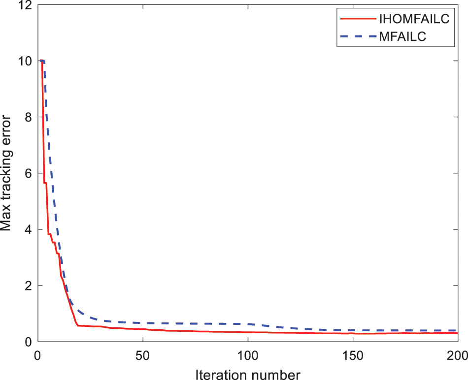
Figure 3: Max tracking error convergence of MFAILC and IHOMFAILC
Based on the model-free adaptive iterative learning control, a novel IHOMFAILC method has been proposed in this paper based on compact form dynamic linearization. When the system is disturbed, the proposed method can still keep track of the desired output. Furthermore, this method can achieve enhanced convergence without many experiments to find a suitable PPD value. Two examples show that the proposed method has good trajectory tracking and disturbance resistance.
Acknowledgement: This work was supported by the Natural Science Foundation of China, under Grant No. 61773183.
Funding Statement: The authors received no specific funding for this study.
Conflicts of Interest: The authors declare that they have no conflicts of interest to report regarding the present study.
References
1. Madadi, E., Söffker, D. (2018). Model-free control of unknown nonlinear systems using an iterative learning concept: Theoretical development and experimental validation. Nonlinear Dynamics, 94(2), 1151–1163. DOI 10.1007/s11071-018-4415-7. [Google Scholar] [CrossRef]
2. Liu, D., Yang, G. H. (2018). Model-free adaptive control design for nonlinear discrete-time processes with reinforcement learning techniques. International Journal of Systems Science, 49(11), 2298–2308. DOI 10.1080/00207721.2018.1498557. [Google Scholar] [CrossRef]
3. Hou, Z. S. (1994). The parameter identification, adaptive control and model-free learning adaptive control for nonlinear systems (Ph.D. Thesis). North-eastern University [Google Scholar]
4. Bu, X. H., Hou, Z. S., Zhang, H. W. (2018). Data-driven multi-agent systems consensus tracking using model-free adaptive control. IEEE Transactions on Neural Network and Learning Systems, 29(5), 1514–1524. DOI 10.1109/TNNLS.2017.2673020. [Google Scholar] [CrossRef]
5. Hou, Z. S., Liu, S., Yin, C. (2016). Local learning-based model-free adaptive predictive control for adjustment of oxygen concentration in the syngas manufacturing industry. IET Control Theory & Applications, 10(12), 1384–1394. DOI 10.1049/iet-cta.2015.0835. [Google Scholar] [CrossRef]
6. Di, S., Li, H. (2018). Model-free adaptive speed control on the travelling wave ultrasonic motor. Journal of Electronic Engineering, 69(1), 14–23. DOI 10.1515/jee-2018-0002. [Google Scholar] [CrossRef]
7. Arimoto, S., Kawamura, S., Miyazaki, F. (1984). Bettering operation of robots by learning. Journal of Robotic Systems, 1(2), 123–140. DOI 10.1002/(ISSN)1097-4563. [Google Scholar] [CrossRef]
8. Treesatayapun, C. (2015). Data input-output adaptive controller based on IF-THEN rules for a class of non-affine discrete-time systems: The robotic plant. Journal of Intelligent & Fuzzy Systems, 28(2), 661–668. DOI 10.3233/IFS-141347. [Google Scholar] [CrossRef]
9. Xiong, Z., Zhang, J. (2003). Product quality trajectory tracking in batch processes using iterative learning control based on time-varying perturbation models. Industrial & Engineering Chemistry Research, 42(26), 6802–6814. DOI 10.1021/ie034006j. [Google Scholar] [CrossRef]
10. Fu, Q., Li, X. D., Du, L. L., Xu, G. Z., Wu, J. R. (2018). Consensus control for multi-agent systems with quasi-one-sided Lipschitz nonlinear dynamics via iterative learning algorithm. Nonlinear Dynamics, 91(4), 2621–2630. DOI 10.1007/s11071-017-4035-7. [Google Scholar] [CrossRef]
11. Zhao, S., Shmaliy, Y. S., Ahn, C. K., Liu, F. (2018). Adaptive-horizon iterative UFIR filtering algorithm with applications. IEEE Transactions on Industrial Electronics, 65(8), 6393–6402. DOI 10.1109/TIE.2017.2784405. [Google Scholar] [CrossRef]
12. Jin, S. T., Hou, Z. S., Chi, R. H., Liu, X. B. (2012). Data-driven model-free adaptive iterative learning control for a class of discrete-time nonlinear systems. Control Theory & Applications, 29(8), 1001–1009. DOI 10.7641/j.issn.1000-8152.2012.8.lcta120438. [Google Scholar] [CrossRef]
13. Bu, X. H., Wang, S., Hou, Z. S. (2019). Model-free adaptive iterative learning control for a class of nonlinear systems with randomly varying iteration lengths. Journal of the Franklin Institute, 356(5), 2491–2504. DOI 10.1016/j.jfranklin.2019.01.003. [Google Scholar] [CrossRef]
14. Hou, Z. S., Jin, S. T. (2013). Model-free adaptive control: Theory and Application. Beijing: Science Press. [Google Scholar]
15. Chi, R. (2006). Adaptive iterative learning control for nonlinear discrete-time systems and its applications. Beijing, China: Beijing Jiao Tong University. [Google Scholar]
16. Zhu, P. P., Bu, X. H., Yu, Q. X., Hou, Z. S., Liang, J. Q. (2020). An improved model-free adaptive iterative learning control algorithm with data quantization. Control Theory & Applications, 37(5), 1178–1184. DOI 10.1002/rnc.5107. [Google Scholar] [CrossRef]
17. Li, J. (2010). Model-free adaptive iterative learning control based on BP algorithm. Microcomputer & Its Applications, 29(22), 83–85. DOI 10.19358/j.issn.1674-7720.2010.22.028. [Google Scholar] [CrossRef]
18. Hua, C. C., Qiu, Y. F., Guan, X. P. (2020). Enhanced model-free adaptive iterative learning control with load disturbance and data dropout. International Journal of Systems Science, 51(11), 2057–2067. DOI 10.1080/00207721.2020.1784492. [Google Scholar] [CrossRef]
19. Bu, X. H., Yu, Q. X., Hou, Z. S. (2019). Model free adaptive iterative learning consensus tracking control for a class of nonlinear multi-agent systems. IEEE Transactions on Systems, 49(4), 677–686. DOI 10.1109/TSMC.2017.2734799. [Google Scholar] [CrossRef]
20. Chi, R. H., Hou, Z. S., Yu, L., Sui, S. L. (2008). Higher order model-free adaptive iterative learning control. Control and Decision, 23(7), 795–798. DOI 10.3321/j.issn:1001-0920.2008.07.015. [Google Scholar] [CrossRef]
21. Chi, R., Hou, Z. S., Jin, S. H., Huang, B. (2018). Computationally efficient data driven higher order optimal iterative learning control. IEEE Transactions on Neural Networks and Learning Systems, 29(12), 5971–5980. DOI 10.1109/TNNLS.2018.2814628. [Google Scholar] [CrossRef]
22. Luo, B., Wu, H. N., Huang, T. (2018). Optimal output regulation for model-free Quanser helicopter with multistep Q-learning. IEEE Transactions on Industrial Electronics, 65(6), 4953–4961. DOI 10.1109/TIE.2017.2772162. [Google Scholar] [CrossRef]
23. Zhao, S., Huang, B., Liu, F. (2017). Linear optimal unbiased filter for time-variant systems without apriori information on initial conditions. IEEE Transactions on Automatic Control, 62(2), 882–887. DOI 10.1109/TAC.2016.2557999. [Google Scholar] [CrossRef]
24. Ai, Q. S., Ke, D., Zuo, J., Meng, W., Liu, Q. et al. (2020). High-order model-free adaptive iterative learning control of pneumatic artificial muscle with enhanced convergence. IEEE Transactions on Industrial Electronics, 67(11), 9548–9559. DOI 10.1109/TIE.2019.2952810. [Google Scholar] [CrossRef]
25. Chi, R. H., Huang, B., Hou, Z., Jin, S. (2017). Data-driven high-order terminal iterative learning control with a faster convergence speed. Robust Nonlinear Control, 28(1), 103–119. DOI 10.1002/rnc.3861. [Google Scholar] [CrossRef]
26. Chi, R. H., Liu, Y., Hou, Z. S., Jin, S. T. (2015). Data-driven Terminal Iterative learning control with high-order learning law for a class of non-linear discrete time multiple-input-multiple output systems. IET Control Theory & Applications, 9(7), 1075–1082. DOI 10.1049/iet-cta.2014.0754. [Google Scholar] [CrossRef]
Cite This Article
 Copyright © 2023 The Author(s). Published by Tech Science Press.
This work is licensed under a Creative Commons Attribution 4.0 International License , which permits unrestricted use, distribution, and reproduction in any medium, provided the original work is properly cited.
 Downloads
 Citation Tools