Computer Modeling in Engineering & Sciences

DOI: 10.32604/cmes.2022.020638

ARTICLE

Numerical Simulation Research on Static Aeroelastic Effect of the Transonic Aileron of a High Aspect Ratio Aircraft

Hongtao Guo, Changrong Zhang, Binbin Lv and Li Yu*

Institute of High Speed Aerodynamics, China Aerodynamics Research and Development Center, Mianyang, 621000, China
*Corresponding Author: Li Yu. Email: yuli@cardc.cc
Received: 04 December 2021; Accepted: 19 January 2022

1  Introduction

For a large aircraft, the heaviest load-bearing component is the wing. Technical indexes, such as aircraft carrying capacity, cruise speed, operation cost and the performance of takeoff and landing, are closely related to the design of wings. Generally, the stiffness of high aspect ratio wings is small, and the aeroelastic phenomenon caused by the interaction between aerodynamic force and wing elastic structure has a significantly influence on the aerodynamic performance and structural safety of the aircraft. Therefore, aeroelasticity is an important problem that must be considered in aircraft design (especially for these aircrafts with high aspect ratio) [1–4]. Aeroelastic design and analysis is an essential part in aircraft design. Most modern high-performance aircrafts have greater flexibility and smaller structural takeoff weight ratio, which makes the static aeroelastic problem more serious. This problem is generally divided into two types, the problem of aerodynamic torsional divergence and load redistribution, and the problem of manipulation efficiency and manipulation reversal. Control efficiency is to study the influence of the elastic deformation of the aircraft structure on rudder surface efficiency, which is an important criterion for wing structure design and aerodynamic design [5].

The structural deformation of the wing has a great impact on the rudder surface efficiency. When the deformation is small, it may reduce the efficiency, while for a large deformation, it may lead to the failure of rudder surface, or even reverse the effect. For example, the “Concorde” aircraft changed by 2° during cruise due to the effect of static aeroelasticity [6]; the rudder efficiency of a high-speed fighter in China reduced to about 1/3 of the rigid body [7] when Ma = 0.9 and the dynamic pressure was 69 kPa; an F/A-18 fighter had experienced aileron reversal during transonic flight. Specifically, the aileron control surface located at the trailing edge of its wing reversed due to the influence of static aeroelasticity, which resulted in a sharp decline in roll maneuverability. The initial modification scheme was to increase the wing stiffness and the aileron length, but the flight test results indicated that the scheme could not solve the problem. Finally, the method of multiple control surfaces was adopted to improve its maneuverability in the transonic range [8]. For swept wings with high aspect ratio, the aileron efficiency deterioration caused by static aeroelastic effect was particularly serious, which could not be ignored. On the one hand, the high aspect ratio wing has large tip deformation, and the aileron is close to the wing tip. On the other hand, due to the wing sweep effect, it is easy for the outflow along the wing span direction to flow on the wing tip. In the early stages of aircraft development, many flight accidents were caused by aileron reversal. In 1927, a British twin-engine aircraft with high aspect ratio had an accident. During the flight, the aileron efficiency was reduced with the increase in the flight speed until aileron reversal occurred. Cox and Pugsley of the Royal Air Force Agency successfully analyzed the accident and put forward the design guidelines to prevent such accidents. Both the C-141 transport aircraft and the Boeing XB-47 bomber also experienced aileron reversal caused by static aeroelasticity during the development stage [9,10]. Therefore, it is necessary to explore the influence of static aeroelasticity on the aileron efficiency of swept wings with high aspect ratio, so as to provide design reference for solving problems of the efficiency reduction of the aircraft control caused by the static aeroelastic deformation.

Considering the time and cost, the industry mostly utilizes the methods of engineering estimation or numerical simulation to analyze static aeroelasticity of aircrafts in the preliminary design stage. Due to the limitations of calculation methods and calculation conditions, aircraft designers mainly estimate the static aeroelastic characteristics of aircraft based on linear aerodynamic theory. For example, NASTRAN and other calculation software widely used in engineering are based on linear small disturbance theory. They can only be applied to subsonic, low supersonic, non-viscous flow conditions and the calculation of static aeroelasticity with simple surface geometry [11–16]. For transonic flow with complex boundary conditions, the aerodynamic results obtained by the traditional methods are far from the real results due to the nonlinearity of aerodynamic force and the interference of shock wave on the viscous boundary layer. Nevertherless, the development of computational fluid dynamics (CFD) and computational structural dynamics (CSD), and that of numerical simulation technology based on Euler equation and Reynolds averaged Navier Stokes equation (RANS equation) in CFD in particular, has been achieved in the past decades. This makes it possible to accurately solve aircraft aeroelastic problems, especially the key transonic aeroelastic problems. Relevant literature has been published in recent years [17–23]. However, most of the studies on the inducement mechanism and key influencing factors of the aileron efficiency reduction of large aircrafts due to the influence of static aeroelasticity at transonic velocity focus on theoretical analysis and qualitative interpretation. There is a lack of analytical research based on high-precision CFD/CSD numerical simulation or high-fidelity wind tunnel test, which leads to the low reference value of existing research outcomes for the engineering field.

In this paper, aiming at the problem of aileron efficiency reduction caused by static aeroelasticity of large aircrafts under transonic and complex aerodynamic conditions, the CFD/CSD fluid-structure coupling numerical simulation method is used to predict the relationship between structural deformation and aerodynamics. The characteristics and mechanism of the effect of wing static aeroelasticity on the efficiency of the aileron are explored. Moreover, the effect of the ‘scissor opening’ gap width between aileron control surface and the main wing surface on aileron efficiency is also discussed.

The main purpose of this paper is to provide technical references for aerodynamic/structural design and wind tunnel experimental model development of large aircrafts.

2  Calculation Methods

2.1 CFD Method

The time-dependent three-dimensional conservative compressible RANS equation was adopted to the governing equation. In the general curvilinear coordinate system (ξ, η, ζ), the dimensionless equation can be expressed as Eq. (1) [22]:

∂Q∂t+∂(F−Fv)∂ξ+∂(G−Gv)∂η+∂(H−Hv)∂ζ=0(1)

where t is time, q is the conserved variable, F, G and H are inviscid vector fluxes, Fv, Gv, and Hv are viscous vector fluxes.

This paper adopted the finite volume method based on grid cell center. The convection term was discretized by the Upwind Flux-Difference-Splitting method based on the three-dimensional Roe scheme. During the reconstruction and interpolation, a minimo limiter was introduced to suppress the nonphysical oscillation near the shock wave based on the MUSCL condition proposed by Van Leer. The viscous term was discretized by the second-order central difference scheme. Implicit LU-SGS method was used for time advance, and SA model was selected as the turbulence model. The material's surface was in an adiabatic no-slip boundary condition, and the far field was in a pressure far-field non-reflecting boundary condition.

2.2 CSD Method

For linear elastic problems, the flexibility influence coefficient method can be used to solve the structural static equations, which can avoid solving the complex structural modal equations. In practice, only a finite number of matrix operations can be performed to obtain the structural elastic deformation. With the advantages of short calculation time and simple processing, it is especially suitable for the study of static aeroelastic problems [24,25]. Generally, the static aeroelastic calculation of large aircraft only considers the elastic deformation of the wing. Other parts, such as the fuselage, engine and its suspension, are assumed to be rigid parts, while the engine and suspension are regarded as following the elastic deformation of the wing. The flexibility coefficient matrix of the wing can be obtained by using a commercial software for structural finite element modeling and calculation, or by ground flexibility matrix measurement experiment. If the aerodynamic load, engine thrust and mass force acting on the wing structure point in three directions are known, the structural statics equation can be used to obtain the elastic deformation displacement of the structural point. The structural statics equation is shown as Eq. (2):

us=CFs(2)

where us is the deformation displacement vector of the structural point, C is the flexibility matrix of the structural point, and Fs is the resultant force vector of aerodynamic force, mass force and engine thrust acting on the structural point.

2.3 Data Interpolation Method between Flow Field and Structure

For general static aeroelastic calculation, CFD is described based on Euler coordinate system, while CSD is described based on Lagrange coordinate system. Therefore, the generation of CFD grids and the establishment of structural models are carried out independently. Thus, it is necessary to introduce data exchange technology between flow field and structure. One is to convert the displacement of structural points into the deformation displacement of grid points in flow field calculation, and the other is to convert the aerodynamic force of CFD grid points into an equivalent force acting on the structural points. The static aeroelastic calculation of large aircraft wings belongs to the small deformation in three-dimensional space. Considering the memory occupancy, calculation efficiency and interpolation accuracy, it is more suitable to use the three-dimensional TPSI method. For the specific calculation formula, please refer to [26].

According to the TPSI method, the structural displacement interpolation matrix H can be obtained from the coordinates of the aerodynamic grid points and the structural point coordinates of the flexibility matrix. Let us and ua be the deformation displacement vector of the structural point and the deformation displacement vector of the aerodynamic grid point, respectively. Then, the relationship between the vectors can be expressed as Eq. (3):

ua=Hus(3)

According to the principle of virtual work, the force interpolation matrix from aerodynamic loads to structural loads and the displacement interpolation matrix from structural points to aerodynamic grid points are transposed to each other. Let Fs and Fa be the force vector of the structural point and the force vector of the aerodynamic grid point, respectively. Then we have Eq. (4):

Fs=HTFa(4)

Therefore, if the load of the aerodynamic grid point Fa on the object surface is known, the deformation displacement vector ua of the aerodynamic grid point on the object surface can be obtained according to Eqs. (2)–(5) [26]:

ua=HCFs=HCHTFa(5)

2.4 Dynamic Mesh Generation Method

After the surface deformation, the original flow field computational grid will no longer be applicable. Therefore, it is necessary to generate a new computational grid. There are two methods for this. One is to regenerate the mesh directly, but this method has low computational efficiency, and usually leads to variation in mesh topology and the number of mesh elements. Its failure to inherit the flow field calculation results of the previous deformation step would result in an excessively long iteration process of static aeroelastic calculation, so this method is not conducive to solving practical engineering problems. The other is to add a certain amount of correction on the original grid. In terms of local areas, the structural deformation of aircrafts is not severe, so this correction method is feasible and has high calculation efficiency. Therefore, this method has been popular in aeroelastic calculation.

In this paper, the unstructured mesh deformation method based on radial basis function was adopted. Wendland's C2 function was selected as the radial basis function, and the greedy algorithm and subspace step-by-step approximation method were used to simplify the object surface interpolation nodes. The grid points near the wall moved with the model wall, and the displacement of grid points far away from the wall was obtained by regional interpolation. This method has high computational efficiency and perfect adaptability to large-scale deformation problems. The quality of the deformed computational grid can be effectively guaranteed.

RBF method is a kind of volume spline function interpolation method, which can be regarded as a three-dimensional extension of surface spline function interpolation method (such as two-dimensional infinite plate spline method) [27]. The interpolation formula can be expressed as Eq. (6):

f(r)=∑i=1nwiφ(‖r−ri‖)+ψ(r)(6)

where ri=(xi,yi,zi) is the known point of displacement and its number is n, φ is the basis function of ‖r−ri‖. Let φ(‖r−ri‖)=‖r−ri‖3 and ψ=b0+b1x+b2y+b3z. Then, the coefficients of the interpolation formula can be obtained by the displacement and equilibrium conditions of the known points ri and di [28], shown as Eq. (7):

f(ri)=di(7-1)

∑i=1nwi=∑i=1nwixi=∑i=1nwiyi=∑i=1nwizi(7-2)

The matrix form of the equations can be expressed as Eq. (8):

[PPT0][Wb]=[d0](8-1)

Φ=[φ11φ12⋯φ1nφ21φ22⋯φ2n⋮⋮⋱⋮φn1φn2⋯φnn](8-2)

where P=[1x1y1z11x2y2z2⋮⋮⋮⋮1xnynzn], W=[w1w2⋮wn], b=[b0b1b2b3], d=[d1d2⋮dn], φij=φ(‖ri−rj‖) [28].

After calculating the coefficients of the interpolation function, for any interpolation point rinter, its displacement can be expressed as dinter=f(rinter).

Theoretically, the displacement of the object surface grid is known, and the displacement of the far-field grid point is set to zero. The displacement of the whole spatial grid can be directly interpolated by using the radial basis function method. However, when the geometric shape of the object surface is complex and the number of the object surface grid is large, the dimension of the matrix in Eq. (8) will be larger, which will seriously decrease the calculation efficiency of grid deformation. Therefore, following the point selection principle of the greedy method, this paper introduced the basic idea of step-by-step approximation of subset in function space, thus effectively relaxing the number limit of radial basis functions. As mentioned in previous section, Eq. (6) was defined on an N-dimensional radial basis function space R(N), which was determined by known displacement nodes (including the object surface and the far field). Considering only the object surface grid points and based on Eq. (6), we can obtain Eq. (9):

ΔS=W(9)

where ΔS is the displacement vector matrix of object surface grid.

Assume that there are N grid nodes in total on the object surface, and M object surface nodes are selected by the greedy method for low-dimensional radial basis function interpolation. The displacement of these M points can be accurately described by the current M-dimensional radial basis function interpolation, but for other object surface grid nodes, there would be errors between their displacement and the results of M-dimensional interpolation. The weight coefficient of the current M-dimensional interpolation is Eq. (10) [29,30]:

W(0)={wS1(0),…,wSM(0)}T(10)

Eq. (10) can be extended to N-dimensional case, written as Eq. (11) [29,30]:

W(0)={wS1(0),…,wSM(0),wSM+1(0),…,wSN(0)}T(11)

where wSM+1(0),…,wSN(0) are zero. Substituting the approximate solution into Eq. (9), we have Eq. (12) [29,30]:

ΔS(0)=ΔS−W(0)(12)

ΔS(0) are not only the residuals of Eq. (9), but also the description error of the current M-dimensional radial basis function interpolation for the node displacement of each object surface grid. If the object of radial basis function interpolation is changed to ΔS(0), we have Eq. (13):

ΔS(0)=W(0)(13)

Object surface grid nodes were selected by the greedy method again, and an L-dimensional radial basis function interpolation pair was constructed in the N-dimensional radial basis function space R(N), which was determined by the object surface displacement nodes. Without losing generality, assuming that there are k duplicate points between the above L points and the previously selected M points, their weight coefficients W(1) are all equal to zero. The residual of Eq. (13) can be expressed as Eq. (14):

ΔS(1)=ΔS(0)−W(1)=ΔS−(W(0)+W(1))(14)

Eq. (14) indicates that the description error of the interpolation on the displacement of object surface nodes is ΔS(1) when Eq. (15) is utilized as the weight coefficient of the radial basis function interpolation determined by the current M + L-K object surface nodes.

W∗=W(0)+W(1)(15)

The above steps were repeated, with a certain number of nodes selected according to the greedy method each time to interpolate the radial basis function of the residual in the previous step, until the residual met the mesh deformation requirements. Then, by superimposing the weight coefficients obtained in this t cycle, the approximate solution of Eq. (9) could be obtained, which is the final radial basis function interpolation coefficient, described as Eq. (16) [29,30]:

W∗=W(0)+W(1)+…+W(t)(16)

The above-mentioned method has obvious advantages over the simple greedy method in terms of computational efficiency. If the dimension of function subspace at all levels is uniformly specified as M, the amount of calculation for 10×M nodes to establish radial basis function interpolation is only 10×M4, while the calculation amount of greedy method alone is (10×M)4 [29,30].

After obtaining the displacement of each point in each grid block edge by interpolation based on the RBF method, the displacement of each point in the grid block surface could be obtained by the TFI method based on the displacement of the corresponding grid block edge. Similarly, the displacement of the internal points of each grid block could also be obtained by the TFI interpolation based on the displacement of the grid block surface [31].

3  Calculation Method Verification

3.1 Computational Model

In this paper, the static aeroelastic numerical calculation based on CFD/CSD coupling method was carried out by using a wing-body configuration semi-model, and the simulation results were compared with the wind tunnel experimental results. The geometric outline of the model is shown in Fig. 1. In the calculation, only the influence of the elastic deformation of the wing was considered. The inside of the wing adopted a beam structure, and the outside was covered with carbon fiber skin. In addition to the main beams of the model, there was a short beam and 13 ribs in the middle part of the inner wing, and the beam frame was connected by corner pieces to support the skin. The rest of the space was filled with a foam shape. The internal structure of the wing is shown in Fig. 2. The structural parameters of the wing were obtained by ground flexibility experiments.

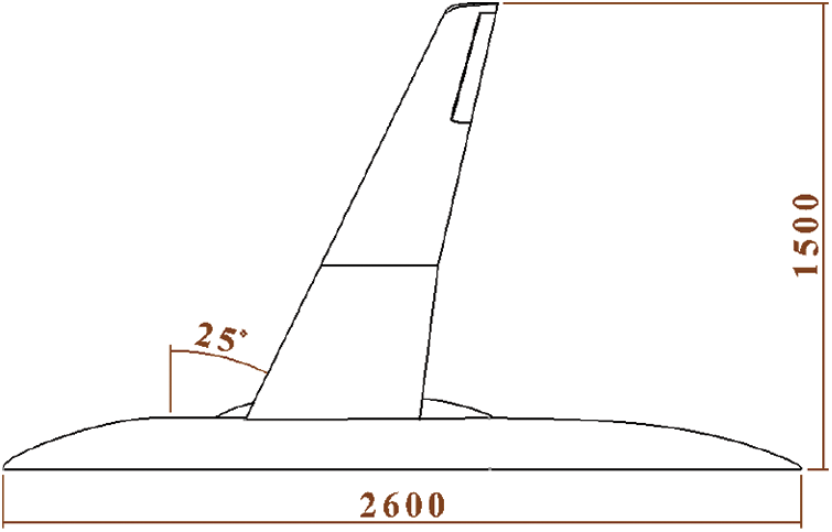
Figure 1: Schematic diagram of the numerical calculation model

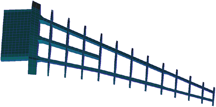
Figure 2: Schematic diagram of the internal structure of the numerical calculation model

The initial computational grid of CFD used multi-partition docking structure grid, and the grid unit size was about 5 million. During grid generation, a layer of boundary layer grid was wrapped around the fuselage and the wing respectively, and the thickness of the first layer of grid was 0.002 ∼ 0.005 mm. In order to apply multigrid technology to accelerate computational convergence, the number of grid points of each structure was strictly controlled according to the rule of 4n + 1 (n is the multiplicity of multigrid). The flow field grid during the initial CFD calculation is presented in Fig. 3.

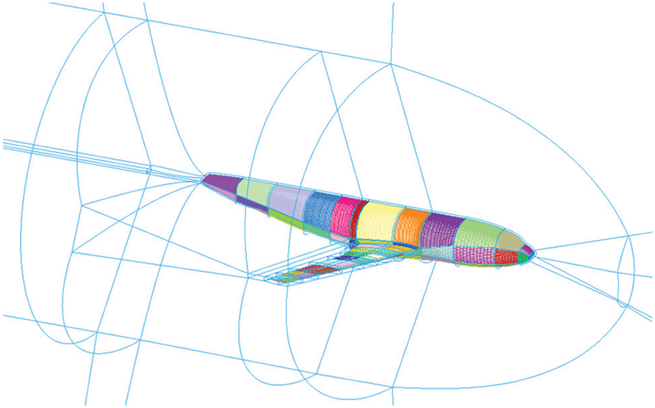
Figure 3: Initial CFD grid

3.2 Calculation Results

The verification calculation state was: Ma = 0.75, q = 35 kPa, Reynolds number Re = 7.1 × 106, and the angle of attack α was −4° ∼ 8°.

Fig. 4 shows the comparison results concerning the wing lift coefficient CL and the bending deformation Δz calculated in this paper and the wind tunnel experiment (the normal deformation of the wing leading edge when α=2°). It should be noticed that there were some inconsistencies between the numerical calculation and the wind tunnel experiment. To be specific, the calculation in this paper used the full turbulence model, while the wind tunnel experiment adopted the free transition mode and it was under the influence of wall interference and support interference. Due to the difficulty of processing composite elastic model, there would be some differences in the three-dimensional shape between the theoretical numerical calculation model and the actual experimental model. Meanwhile, limited by the current technical means, it is not possible to remedy the lack of turbulence simulation and inaccurate simulation of separation characteristics in CFD, as well as the possible nonlinear wing deformation. Nonetheless, the calculated results in this paper were generally consistent with the wind tunnel experiment results. There was a roughly fixed systematic error between CL obtained by the wind tunnel experiment and numerical calculation. The error of Δz mainly lied in the large deformation range of the wing tip.

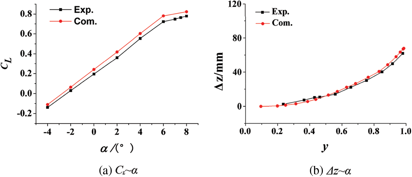
Figure 4: Comparison between numerical calculation and wind tunnel experiment results

4  Numerical Simulation Analysis of Aileron Static Aeroelasticity

The wing-body configuration full model could be obtained by adding the other symmetrical half to the semi-model in Fig. 1 along the longitudinal direction of the fuselage. Based on the above-mentioned static aeroelastic numerical simulation method, the static aeroelastic effect of transonic ailerons was studied. The contents and working conditions of the numerical calculation are shown in Table 1. In the numerical simulation of static aeroelasticity, the fuselage was treated as a rigid body, and only the elastic deformation of wings and ailerons was considered. In addition, the aileron control surface was elastically supported in terms of the rotational degrees of freedom. In other words, the rotational stiffness of the ailerons was considered in the calculation of this paper.

4.1 Effect of Aileron Efficiency

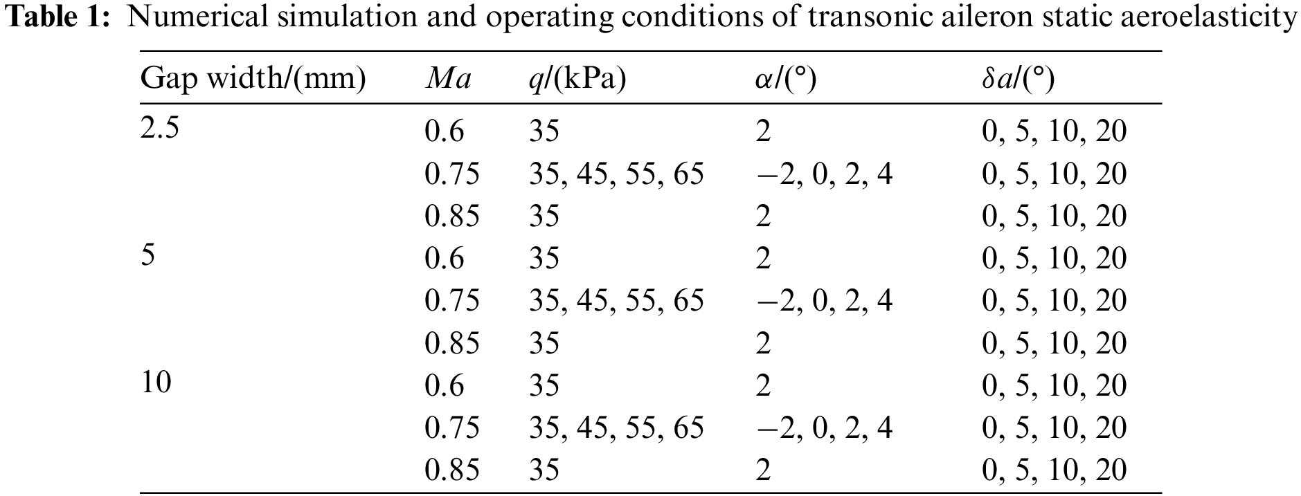
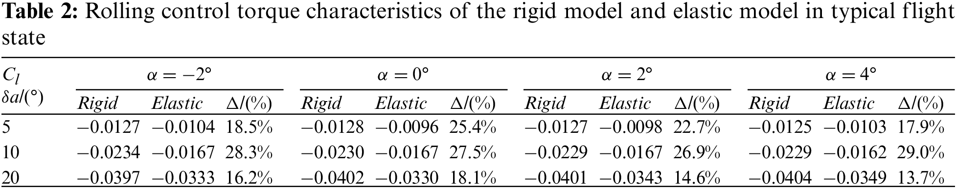
Figs. 5, 6, and Table 2 show the rolling control torque characteristics of rigid and elastic models in typical flight state (Ma = 0.75, q = 35 kPa). It can be seen that when the aileron deflected, the rolling control torque coefficient Cl of the elastic model was significantly smaller than that of the rigid model at different flight angles of attack, due to the action of static aeroelasticity. This indicates that the efficiency of the aileron was significantly decreased. For example, when α = 2°, δa = 10°, and ΔCl = 0.0062, the rolling control torque coefficient of the elastic model decreased by 26.9% compared with that of the rigid model. In addition, a phenomenon can be found in Fig. 5 and Table 2: with the change in aileron control surface deflection, the influence degree of static aeroelasticity was not the same. Before δa = 10°, the influence gradually increased; when δa = 10° ∼ 20°, the influence increased to the maximum and tended to balance. The reason for this phenomenon is: the aileron control surface had reached its stall range near 20°, so the force and moment generated by the aileron control surface would remain unchanged at this time; the deformation of the main airfoil of the elastic model was affected by the load on the aileron control surface, so the elastic deformation of the main airfoil would also remain unchanged, and thus the rolling moment would remain unchanged at δa = 20°. Therefore, the rolling moment coefficients of the elastic model and rigid model remained parallel in the range of δa = 10° ∼ 20°.

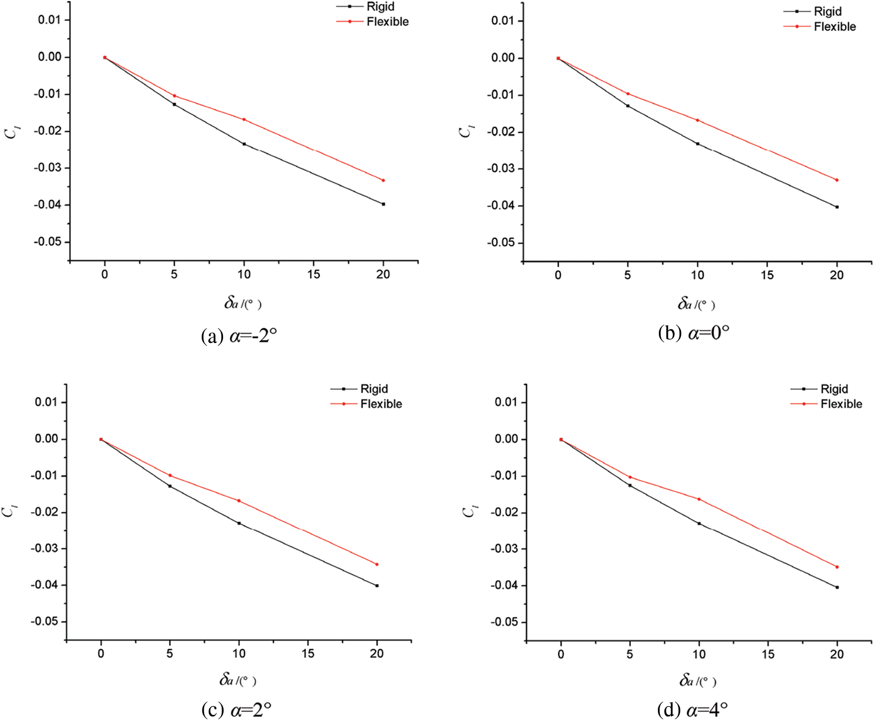
Figure 5: Comparison of rolling moment characteristics between the rigid model and elastic model in typical flight state

Figure 6: The rolling moment characteristics of the rigid model and elastic model varied with the angle of attack in typical flight state

In order to better reflect the difference in the influence of static aeroelasticity on aileron efficiency at different angles of attack, Fig. 7 shows the variation in Cl of the rigid model and elastic model with angle of attack. Within the range of the calculation state, the influence of angle of attack on rigid model or elastic model was very small, and the aileron efficiency did not significantly change with the angle of attack.

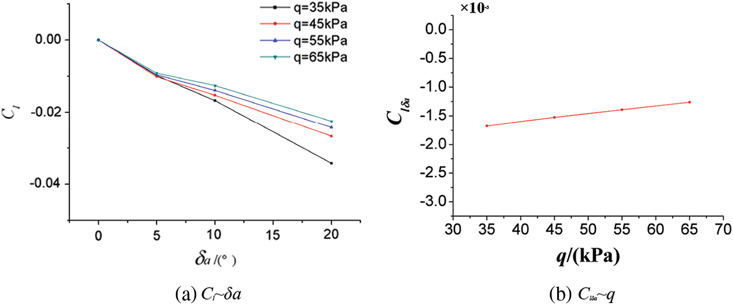
Figure 7: Effect of dynamic pressure on aileron efficiency of elastic model

(1)   Effect of dynamic pressure on aileron efficiency of elastic model

Fig. 7 shows that when Ma = 0.75, α = 2°, the Cl of the elastic model varied with the deflection of the aileron control surface under different velocities and pressures, and the aileron efficiency (Clδa) varied with dynamic pressure. The dynamic pressure had a significant influence on the aileron efficiency of the elastic model. With the increase in dynamic pressure, the aileron efficiency of the elastic model decreased gradually. For example, when 0° ≤ δa ≤ 10°, aileron efficiency of the elastic model was reduced by 27% compared to that of the rigid model when q = 35 kPa, while the efficiency reduction percentage reached 45% when q = 65 kPa.

(2)   Influence of Mach number on the static aeroelastic effect of aileron

Fig. 8 shows the change curves of Cl of the rigid model and elastic model with the aileron control surface skewness δa under different Mach numbers when q = 35 kPa and α = 2°. Fig. 9 presents the change of Clδa with the Mach number.

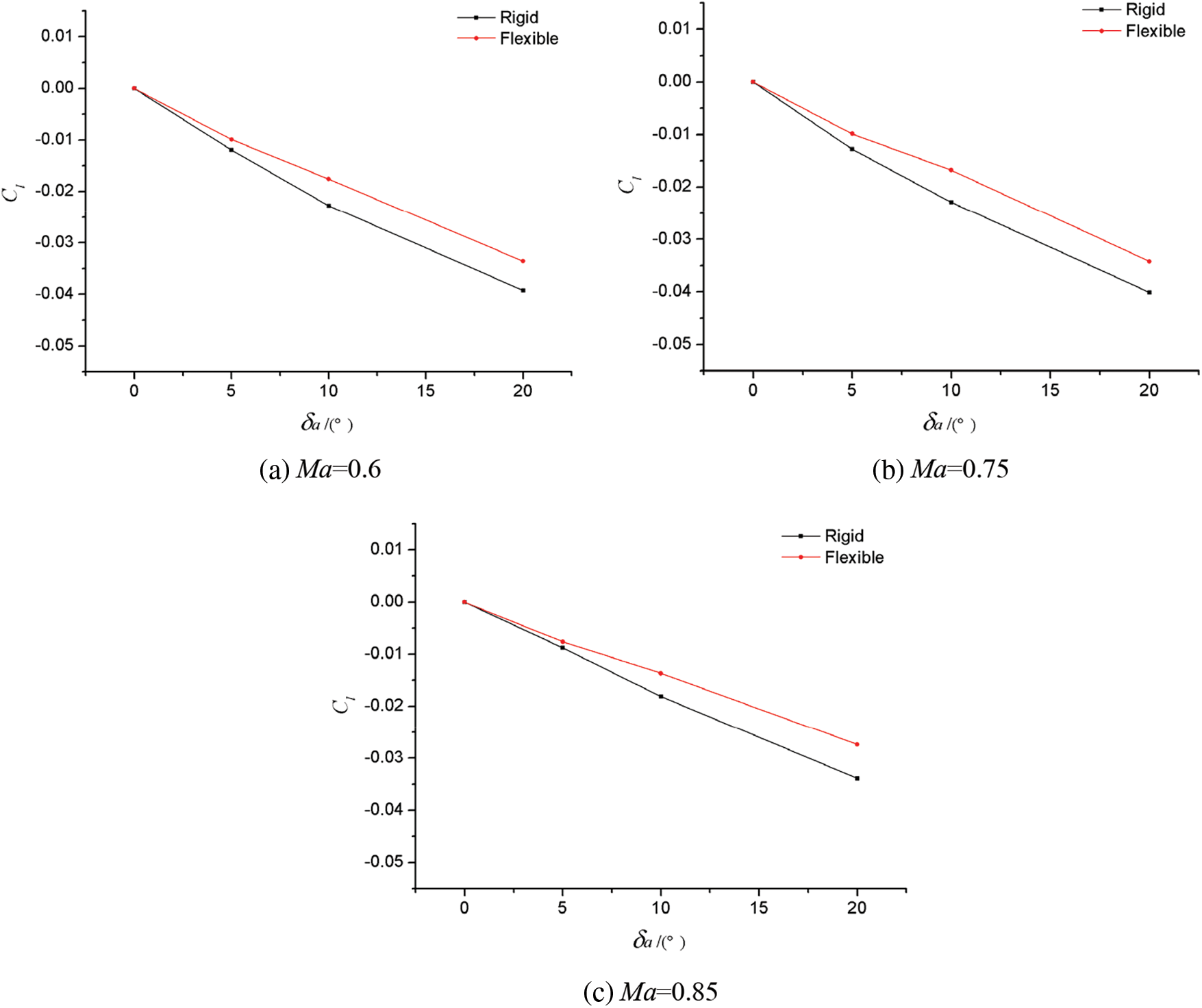
Figure 8: Comparison of rolling torque characteristics between rigid and elastic models with different Mach numbers

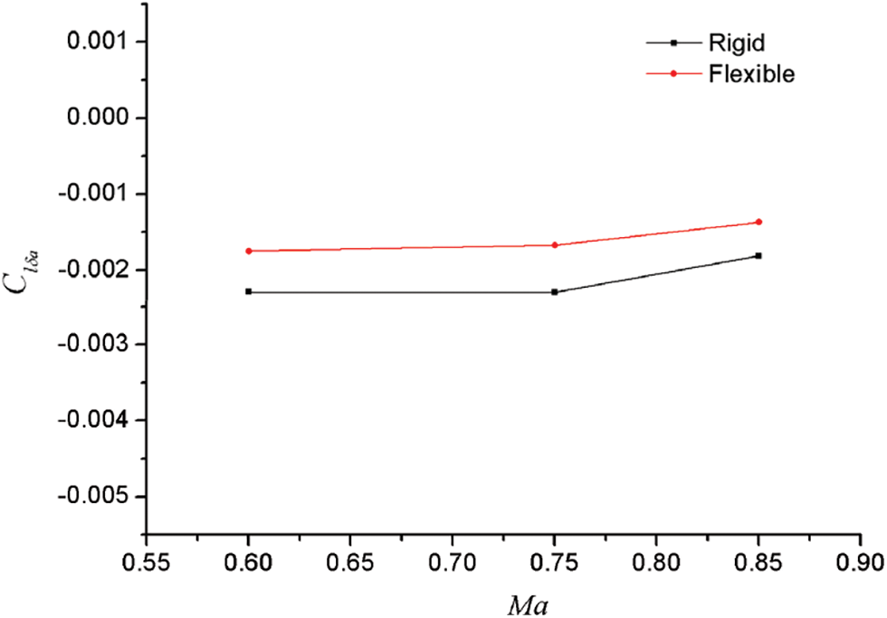
Figure 9: Effect of Mach number on aileron efficiency characteristics

It can be found from Fig. 8 that compared to that of the rigid model, the rolling control torque of the elastic model decreased under different Mach numbers, and the greater the aileron deflection, the greater the decrease. From Fig. 9, we can see that the static aeroelastic effect could reduce the aileron efficiency (Clδa was obtained according to the linear law with the range of 0° ≤ δa ≤ 10°). However, with the change in Mach numbers, the reduction degree and change law of aileron efficiency were generally similar, and there was no fundamental difference between different Mach numbers.

4.2 Mechanism Analysis of Aileron Efficiency Reduction

According to the previous analysis and discussion, for the swept wing with high aspect ratio, the rolling control force is weakened and the aileron efficiency is significantly reduced by the effect of static aeroelasticity. In this section, the reasons for the reduction of aileron efficiency will be analyzed based on the numerical simulation results of aileron geometric deformation, surface pressure coefficient and flow characteristic data, and the mechanism of the aileron static aeroelastic effect will be explained.

Fig. 10 shows the comparison of the elastic deformation effects of ailerons between rigid model and elastic model when Ma = 0.75, q = 35 kPa, α = 2°, and δa = 10°. It can be found that due to the difference in aerodynamic load caused by the differential deflection of the left and right ailerons, there was a significant difference in the overall elastic deformation of the left and right wings. For the sections marked by the “red line” in the figure (the two sections were symmetrical, respectively located at the position of 94% of the half-span wing), according to the numerical calculation results in this paper, the difference in aileron deflection between the elastic model and the rigid model was: (Δδa)left = −1.5°, (Δδa)right = −4.9°. In other words, the static aeroelastic deformation reduced the deviation difference between the left and right aileron control surfaces. In the next section, the paper will further analyze and compare the difference in surface pressure coefficients and surface flow characteristics of the rigid model and the elastic model, and uncover the essential reasons for the reduced efficiency of the elastic model ailerons.

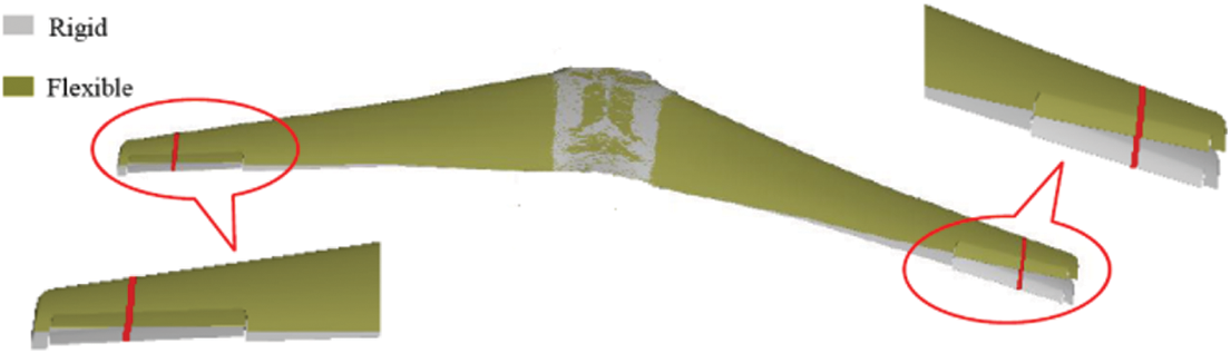
Figure 10: 3D rendering of wing/aileron elastic deformation

Fig. 11 shows that when Ma = 0.75, q = 35 kPa, α = 2°, and δa = 10°, the rigid model and the elastic model were located at the 95% of the half-span wing, as identified by the “red line” in Fig. 10. Fig. 12 presents the cloud diagram of the wing surface pressure coefficient distribution and the surface streamline distribution near the aileron control surface under corresponding conditions of Fig. 10.

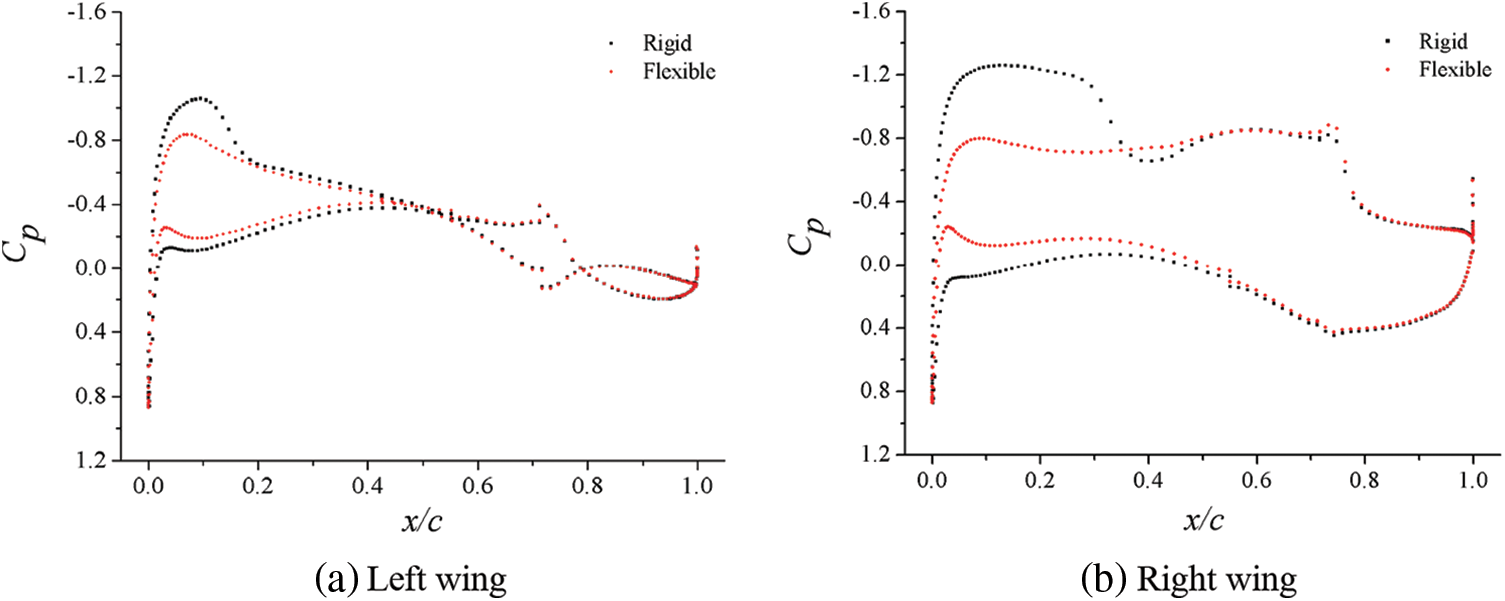
Figure 11: Surface pressure coefficients at typical locations of airfoils of rigid and elastic models

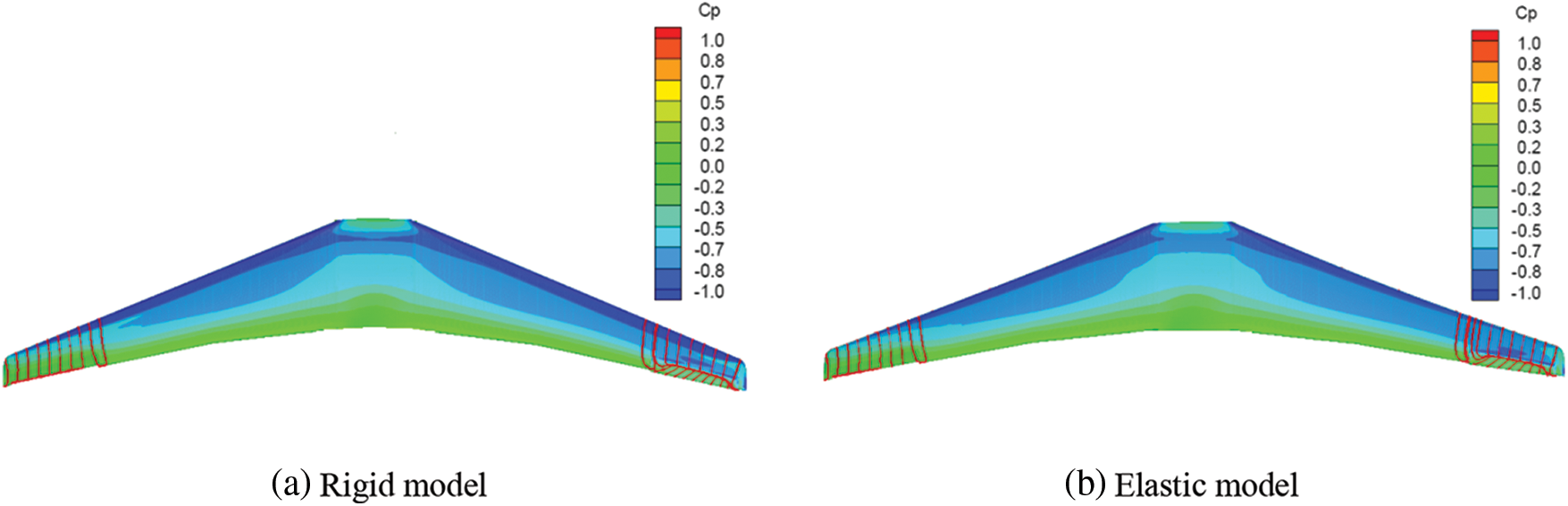
Figure 12: Nephogram of surface pressure coefficients of airfoils of rigid and elastic models

At these two sections, pressure distributions of the rigid model and the elastic model were obviously different along the chord length of the wing. Specifically, the pressure load of the rigid model was significantly greater than that of the elastic model, and this difference was particularly obvious at the right wing (observed along the course) near the leading edge of the wing tip (torsional deformation caused the weakening of the shock wave and downward deflection of right aileron, which in turn led to greater torsional deformation). It is worth noting that the largest difference in pressure distribution between rigid model and elastic model did not appear in the chord position of the corresponding aileron control surface, but mainly existed before 50% of the wing chord length. When it was close to the aileron control surface, the difference in pressure distribution was rather small. After careful analysis, there are two reasons for this phenomenon. First, when the aileron control surface deflected and bore aerodynamic load, it was equivalent to a large concentrated load at the aileron position for the whole wing. Since this concentrated load was farther from the elastic axis of the wing than that of the aileron, the elastic deformation of the wing caused by the aileron control torque would be greater than that of the aileron control surface itself. In other words, the aileron control surface acted as a “lever” (the elastic deformation of the main wing occurred after “prying” under aerodynamic load). The inconsistent elastic deformation of the main wing surfaces of the left and right wings caused by its differential deflection, rather than the large elastic deformation of the aileron control surface, was the main reason for the reduction in the rolling control efficiency. With the increase in the elastic deformation, the local angle of attack changed greatly, which led to a larger difference in the pressure distribution. Therefore, it is not difficult to understand the pressure distribution difference in the main wing surface shown in Fig. 10. Second, for the wing sections of the rigid model and elastic model marked by the “red line” in Fig. 10, they were equivalent to two similar airfoils with different angles of attack. When the aileron deflection did not equal to zero, it was equivalent to a large camber in the rear half of the airfoil. Therefore, when the angle of attack of the two airfoils was not much different, the difference in attack angle and flow at the rear of the airfoil were relatively small due to its large curvature.

According to the comparative analysis of Figs. 11 and 12, difference existed in the surface pressure distribution and flow characteristics near the aileron control surface between the rigid model and the elastic model, but the cause for the difference in rolling control characteristics or aileron efficiency between the two models was not clear. This is because the rolling control characteristics or aileron efficiency of the two models would be consistent with each other, if the load difference between the left and right ailerons of these models was exactly equal. Therefore, the surface pressure coefficients of the left and right ailerons of the rigid model and the elastic model under corresponding conditions were drawn in one diagram, respectively, as shown in Fig. 13. The difference between the areas surrounded by the “red curve” and the “black curve” in the diagrams reflected the pressure load difference between the corresponding left and right sections. It can be clearly seen from the figure that the difference between the corresponding sections of the rigid model and the elastic model was inconsistent. This is the essential reason for the reduction in rolling control characteristics or aileron efficiency of the elastic model caused by static aeroelasticity effect. In conclusion, the deflection of aileron control surface produced lift increment, and caused torsional deformation of elastic wing, which reduced the control surface efficiency and left and right lift increment.

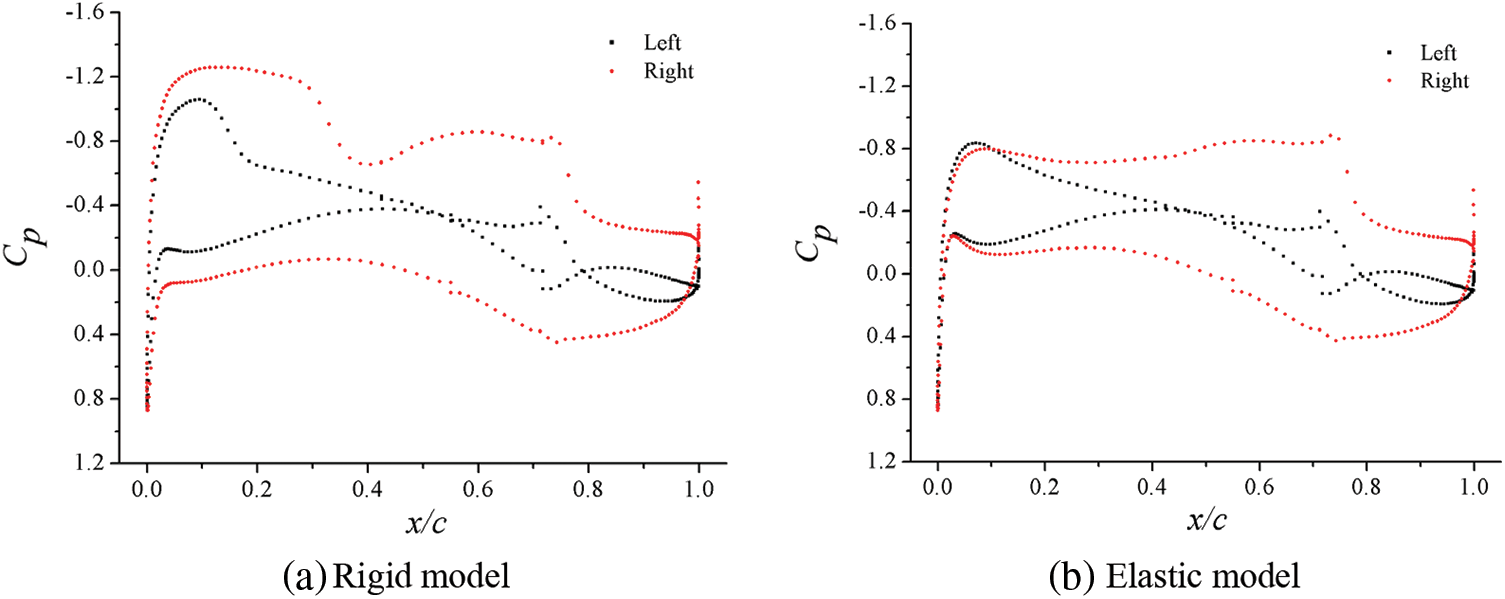
Figure 13: Nephogram of surface pressure coefficients of airfoils of rigid and elastic models

4.3 Influence of Aileron Control Surface Gap

Whether for real aircraft or wind tunnel experimental model, to realize the differential deflection of aileron control surface, a certain gap must be left between control surface and main wing surface to avoid interference during control surface deflection. Reference [32] clearly pointed out that the gap of the control surface has an impact on the aerodynamic characteristics of the aircraft (mainly on the efficiency of the control surface). Thus, it is necessary to pay attention to simulating the gap of the control surface in the shape simulation. However, the model and Reynolds number are small, and the viscous effect of air flow are relatively large, which may not show the gap effect when the gap is too small (such as less than 0.2 mm). On the contrary, if the gap is too large, it will affect the aerodynamic characteristics. At present, there is no strict experimental research conclusion on how to simulate the gap, and most studies only slightly enlarge the exceedingly small gap after reduction. Therefore, in order to provide guidance for the design of subsequent static aeroelastic wind tunnel experiment models, the influence of the aileron control surface gap will be studied and analyzed in this section. Generally, the gap at the leading edge of the aileron control surface leaves only a small clearance in the model design, and there is no geometric interference. And the gap can be blocked with putty or adhesive tape during the experiment. However, as shown in Fig. 14, when the aileron deflection is not zero, the gap structure between the aileron and the main wing will be similar to a “scissor opening”, and this “scissor opening” gap is difficult to simulate accurately in the experiment. Therefore, this paper focused on the effect of the “scissor opening” gap on both sides.

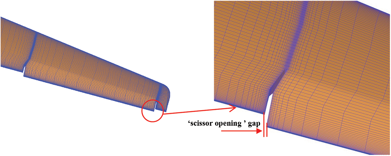
Figure 14: Schematic diagram of aileron “scissor opening”

This paper mainly studied the influence of three kinds of “scissor opening” gaps with different widths, namely 2.5, 5, and 10 mm. Fig. 15 shows the curves of Cl changed with the gap width at different attack angles when Ma = 0.75, q = 35 kPa, and δa = 10°. Fig. 16 shows the curves of Cl changed with the gap width under different dynamic pressure when Ma = 0.75, α = 2°, and δa = 10°. Fig. 17 shows the curves of Cl changed with the gap width at different Mach numbers when q = 35 kPa, α = 2°, and δa = 10°.

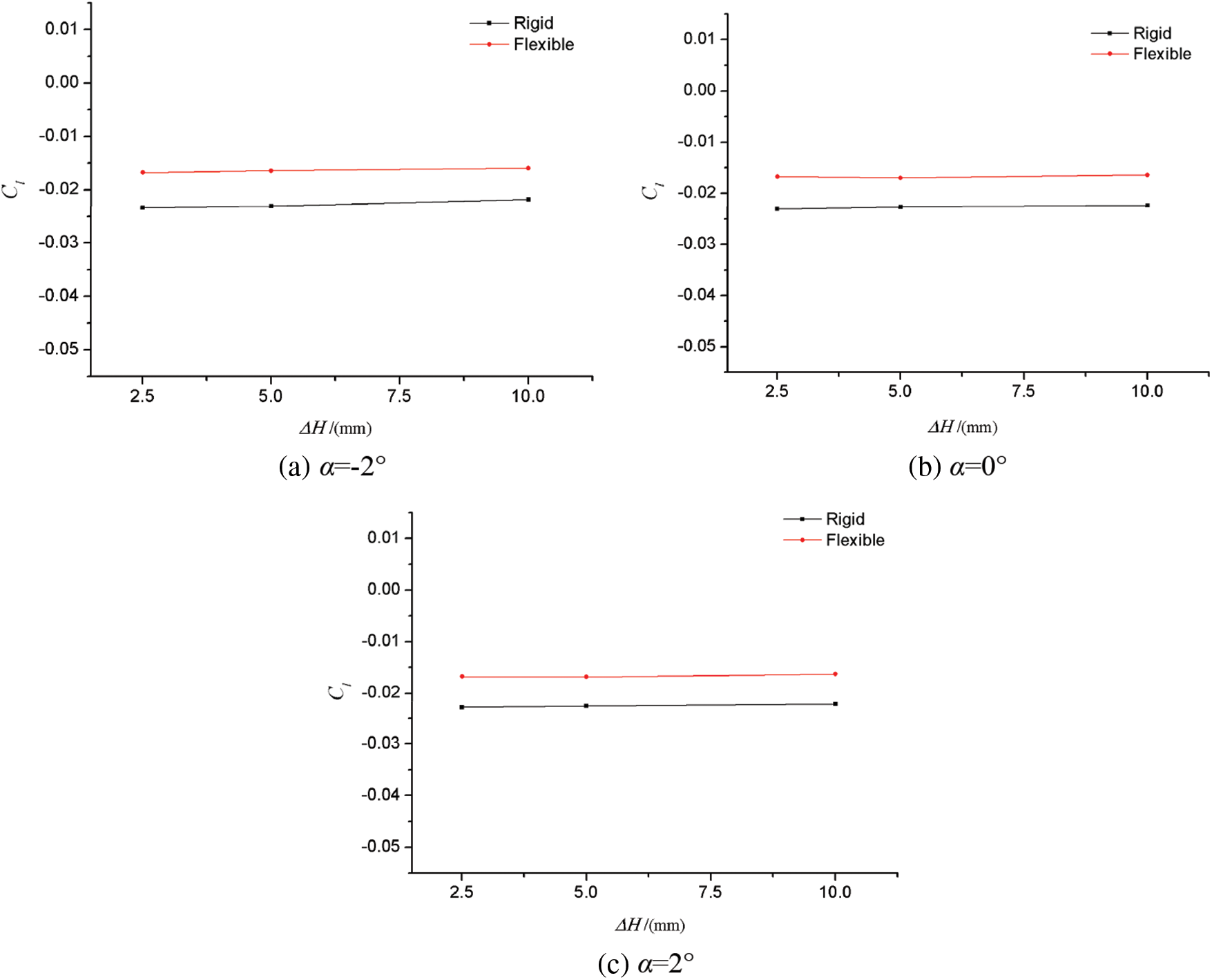
Figure 15: Effect of gap width on aileron rolling torque characteristics at different angles of attack

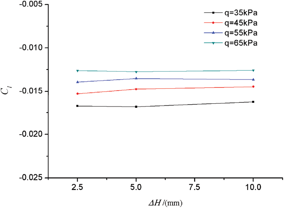
Figure 16: Influence of gap width on aileron rolling torque characteristics at different speeds

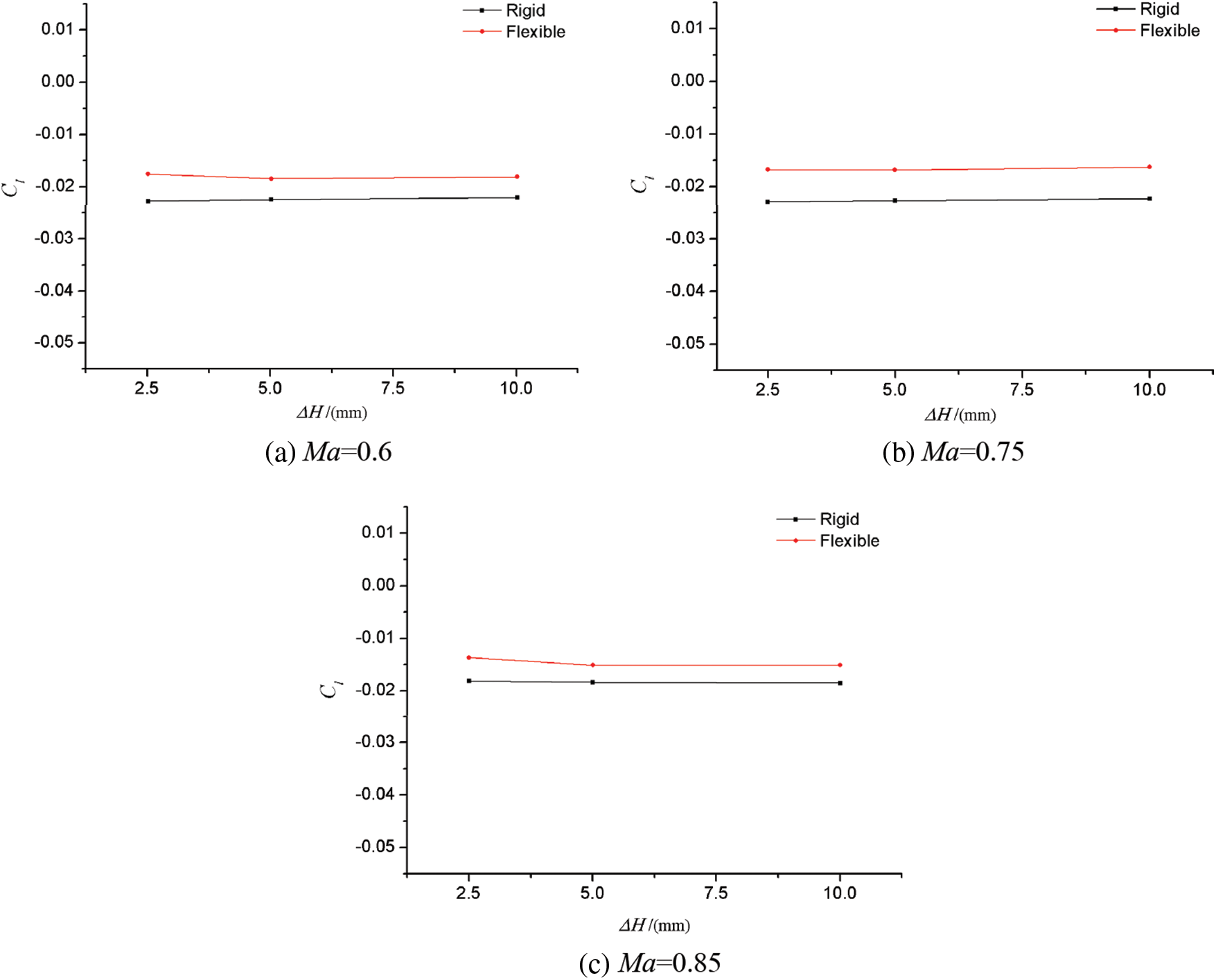
Figure 17: Effect of gap width on aileron rolling torque characteristics at different Mach numbers

It can be seen from the figures that under different angles of attack, dynamic pressure and Mach numbers, the gap width of “scissor opening” had no obvious effect on the static aeroelastic effect of aileron. In other words, although the gap width of the control surface would affect the aileron control characteristics of the rigid model or the elastic model, it had no effect on the difference between the two models. Therefore, in order to study the static aeroelastic effect or influence degree of the aileron, the simulation requirements for the “scissor opening” gap of the aileron control surface can be relaxed when designing the static aeroelastic model of the aileron.

5  Conclusion

This paper has investigated the static aeroelastic effect of large aircraft ailerons based on the high-precision CFD/CSD coupling numerical simulation method. The results have shown that the influence of static aeroelasticity on the rolling control of high aspect ratio swept wings cannot be ignored, because it can significantly change the aileron efficiency. The findings are summarized as follows:

(1)   Decreasing the rolling control torque leads to the reduction in aileron efficiency. Near the design cruise point, the rolling control torque of the elastic model decreases by 26.9% compared with that of the rigid model when δa = 10°.

(2)   In the range of medium and small angles of attack, the flight attack angle and Mach number have little influence on the static aeroelastic effect of ailerons. The flight dynamic pressure is an important parameter affecting the static aeroelastic effect of ailerons. And the higher the dynamic pressure, the lower the aileron efficiency.

(3)   Through the comprehensive analysis of the geometric deformation, surface pressure distribution, and surface flow characteristics of the swept wings, it is found that the differential deflection of the aileron control surface will lead to the corresponding geometric deformation of the wing. The aerodynamic load generated after the deformation will offset the load difference between the left and right ailerons, thereby resulting in a significant reduction in the aileron efficiency.

(4)   For the typical high-speed static aeroelastic model studied in this paper, the “scissor opening” gap width of the aileron has little effect on its static aeroelastic effect in the range of 2.5–10 mm.

Funding Statement: The authors received no specific funding for this study.

Conflicts of Interest: The authors declare that they have no conflicts of interest to report regarding the present study.

This work is licensed under a Creative Commons Attribution 4.0 International License, which permits unrestricted use, distribution, and reproduction in any medium, provided the original work is properly cited.