| Computer Modeling in Engineering & Sciences |
DOI: 10.32604/cmes.2022.017272
ARTICLE
Some Identities of the Degenerate Poly-Cauchy and Unipoly Cauchy Polynomials of the Second Kind
1Department of Mathematics, Faculty of Science, University of Tabuk, Tabuk, 71491, Saudi Arabia
2Department of Mathematics and Natural Sciences, Prince Mohammad Bin Fahd University, Al Khobar, 31952, Saudi Arabia
3Department of Mathematics and Statistics, College of Science, Taif University, Taif, 21944, Saudi Arabia
*Corresponding Author: Ghulam Muhiuddin. Email: chishtygm@gmail.com
Received: 27 April 2021; Accepted: 11 February 2022
Abstract: In this paper, we introduce modified degenerate polyexponential Cauchy (or poly-Cauchy) polynomials and numbers of the second kind and investigate some identities of these polynomials. We derive recurrence relations and the relationship between special polynomials and numbers. Also, we introduce modified degenerate unipoly-Cauchy polynomials of the second kind and derive some fruitful properties of these polynomials. In addition, positive associated beautiful zeros and graphical representations are displayed with the help of Mathematica.
Keywords: Modified degenerate polyexponential functions; modified degenerate polyexponential Cauchy (or poly-Cauchy) polynomials of the second kind; degenerate unipoly-Cauchy polynomials of the second kind
Recently, many mathematicians, specifically Carlitz [1,2], Kim et al. [3–5], Kim et al. [6,7], Sharma et al. [8,9], Khan et al. [10–13], and Muhiuddin et al. [14–17] have studied and added diverse degenerate versions of many special polynomials and numbers (like as degenerate Bernoulli polynomials, degenerate Euler polynomials, degenerate Daehee polynomials, degenerate Fubini polynomials, degenerate Stirling numbers of the first and second kind, and so on). In this paper, we focus on modified degenerate polyexponential Cauchy (or poly-Cauchy) polynomials and the numbers of the second type. The purpose of this paper is to introduce a degenerate model of the poly-Cauchy polynomials and numbers of the second type, the so-called degenerate poly-Cauchy polynomials, and numbers of the second type, constructed from the degenerate polyexponential feature. We derive some express expressions and identities for the one’s numbers and polynomials.
Let
In the case when
The Bernoulli polynomials of order
For
We note that
For
By (4) and binomial theorem, we have
where
The degenerate Bernoulli polynomials are defined by (see [1,2])
On putting x = 0,
The degenerate Cauchy polynomials
Letting
In the year 2017, Kim [24] introduced and studied the new class of degenerate Cauchy polynomials
At the point when
The degenerate Daehee polynomials
On setting
The degenerate Bernoulli polynomials of the second kind are defined by (see [6])
Letting
For
Note that
For
We note that
In this paper, Section 3 incorporates the definition of degenerate poly-Cauchy polynomials of the second kind and a preliminary study of these polynomials. Section 4 is a consequence of the definition of the degenerate unipoly-Cauchy polynomials and unipoly polynomials combined with their properties and special cases. Finally, some computational values of degenerate poly-Cauchy polynomials of the second kind are given in Section 5.
2 Degenerate Poly-Cauchy Polynomials and Numbers of the Second Kind
In this segment, we introduce degenerate poly-Cauchy polynomials of the second kind, derived with the aid of modified degenerate polyexponential functions and some identities of these polynomials.
Recently, Kim et al. [4] delivered the modified degenerate polyexponential function defined by
Thus, by
The modified degenerate polyexponential Genocchi (or poly-Genocchi) polynomials are defined by Kim et al. to be (see [7])
At the point when
By the above definitions, we introduce modified degenerate polyexponential Cauchy (or poly-Cauchy) polynomials of the second kind as
When
Theorem 2.1. Let j be non negative number. Then
Proof. Using (11) and (18), we have
Therefore, by (15) and (20), we obtain the result (19).
Corollary 2.1. Let j be non negative number. Then
Theorem 2.2. Let j be non negative number and
Proof. Recall from (18), we have
Thus by (18) and (22), the proof is completed.
Theorem 2.3. Let
Proof. Consider (15), we have
which complete the proof.
Corollary 2.2. Let
Theorem 2.4. The following result holds true
Proof. Let us define the function
For any
Eq. (27) can be written as
In view of (26) and (27), we have
By (28), we obtain the result.
Theorem 2.5. Let j be non-negative number. Then
Proof. By changing z with
On the other hand, we see that
In view of (29) and (30), we obtain the result.
Theorem 2.6. Let
Proof. Consider the Eq. (18), we have
The complete of the Proof.
Corollary 2.3. Let
Theorem 2.7. Let j be non-negative number. Then
Proof. We observe that
Therefore, by (15) and (34), we acquire the desired result.
Theorem 2.8. Let j be non-negative number. Then
Proof. Consider the following expression:
From Eq. (35), we have
Thus, by (36) and (37), we complete the proof.
3 DegenerAte Unipoly-Cauchy Polynomials of the Second Kind
In this section, we introduce degenerate unipoly-Cauchy polynomials of the second kind by using degenerate unipoly function and derive the relationships between degenerate Daehee polynomials and degenerate Cauchy polynomials of the second kind.
In [25], Dolgy and Khan introduced degenerate unipoly function given by
Note that, we have
is the modified degenerate polyexponential function, where
It is clear that
are called the unipoly function attached to polynomials p(x) (see [3]).
From (40), we have
is the ordinary polylogarithm function.
By using (15) and (38), the degenerate unipoly-Cauchy polynomials of the second kind is given by the following generating function
In the case when
Theorem 3.1. Let
Proof. On taking
In view of (43), we obtain the result.
Theorem 3.2. Let j be non-negative number. Then
Proof. Consider the Eq. (42), we have
By (42) and (45), we complete the proof.
Corollary 3.1. Let
Theorem 3.3. Let
Proof. Recall from (42), we see that
Thus, by (47), we get the desired result.
Theorem 3.4. Let
Proof. Using (42), we have
In view of (49), we complete the proof.
4 Computational Values and Graphical Representation of Degenerate Poly-Cauchy Polynomials of the Second Kind
In this section, sure numerical computations are carried out to calculate sure contributors of the degenerate poly-Cauchy polynomials of the second kind and display some graphical representations. The first six individuals of
To show the behavior of
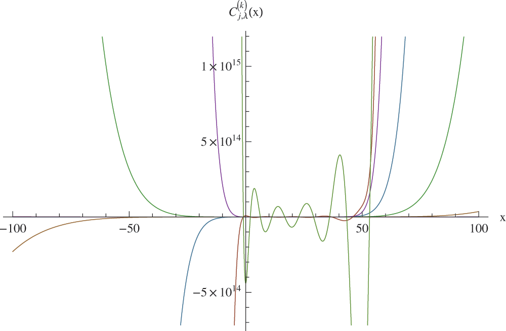
Figure 1: Graph of
In this paper, we have presented the degenerate poly-Cauchy numbers and polynomials of the second kind and discussed, in particular, some interesting series representations. We have deduced some relevant properties by using the structure and the relations satisfied by the recently degenerate polyexponential functions. Section 3 incorporates the definition of degenerate poly-Cauchy polynomials of the second kind and a preliminary study of these polynomials. Section 4 is a consequence of the definition of the degenerate unipoly-Cauchy polynomials and unipoly polynomials combined with their properties and special cases. Finally, some computational values of degenerate poly-Cauchy polynomials of the second kind are given in Section 5.
Acknowledgement: The authors wish to express their appreciation to the reviewers for their helpful suggestions which greatly improved the presentation of this paper.
Funding Statement: This work was supported by the Taif University Researchers Supporting Project (TURSP-2020/246), Taif University, Taif, Saudi Arabia.
Conflicts of Interest: The authors declare that they have no conflicts of interest to report regarding the present study.
1. Carlitz, L. (1967). A degenerate staudt-clausen theorem. Archiv der Mathematik, 7, 28–33. DOI 10.1007/BF01900520. [Google Scholar] [CrossRef]
2. Carlitz, L. (1979). Degenerate Stirling, Bernoulli and Eulerian Numbers. Utilitas Mathematica, 15, 51–88. [Google Scholar]
3. Kim, D. S., Kim, T. (2019). A note on polyexponential and unipoly functions. Russian Journal of Mathematical Physics, 26, 40–49. DOI 10.1134/S1061920819010047. [Google Scholar] [CrossRef]
4. Kim, T., Kim, D. S. (2020). Degenerate polyexponential functions and degenerate Bell polynomials. Journal of Mathematical Analysis and Applications, 487(2), 1–15. DOI 10.1016/j.jmaa.2020.124017. [Google Scholar] [CrossRef]
5. Kim, T., Kim, D. S. (2020). Note on the degenerate gamma function. Russian Journal of Mathematical Physics, 27(3), 352–358. DOI 10.1134/S1061920820030061. [Google Scholar] [CrossRef]
6. Kim, T., Kim, D. S., Kim, H. Y., Kwon, J. (2020). Some results on degenerate Daehee and Bernoulli numbers and polynomials. Advances in Difference Equations, 2020, 311. DOI 10.1186/s13662-020-02778-8. [Google Scholar] [CrossRef]
7. Kim, T., Kim, D. S., Kwon, J., Kim, H. Y. (2020). A note on degenerate Genocchi and poly-Genocchi numbers and polynomials. Journal of Inequalities and Applications, 2020, 110. DOI 10.1186/s13660-020-02378-w. [Google Scholar] [CrossRef]
8. Sharma, S. K., Khan, W. A., Araci, S., Ahmed, S. S. (2020). New type of degenerate Daehee polynomials of the second kind. Advances in Difference Equations, 428, 1–14. DOI 10.1186/s13662-020-02891-8. [Google Scholar] [CrossRef]
9. Sharma, S. K., Khan, W. A., Araci, S., Ahmed, S. S. (2020). New construction of type 2 of degenerate central Fubini polynomials with their certain properties. Advances in Difference Equations, 587, 1–11. DOI 10.1186/s13662-020-03055-4. [Google Scholar] [CrossRef]
10. Khan, W. A., Muhiuddin, G., Muhyi, A., Al-Kadi, D. (2021). Analytical properties of type 2 degenerate poly-Bernoulli polynomials associated with their applications. Advances in Difference Equations, 2021(420), 1–18. DOI 10.1186/s13662-021-03575-7. [Google Scholar] [CrossRef]
11. Khan, W. A., Muhyi, A., Ali, R., Alzobydi, K. A. H., Singh, M. et al. (2021). A new family of degenerate poly-Bernoulli polynomials of the second kind with its certain related properties. AIMS Mathematics, 6(11), 12680–12697. DOI 10.3934/math.2021731. [Google Scholar] [CrossRef]
12. Khan, W. A., Acikgoz, M., Duran, U. (2020). Note on the type 2 degenerate multi-poly-Euler polynomials. Symmetry, 12, 1–10. DOI 10.3390/sym12101691. [Google Scholar] [CrossRef]
13. Khan, W. A., Ali, R., Alzobydi, K. A. H., Ahmed, A. (2021). A new family of degenerate poly-Genocchi polynomials with its certain properties. Journal of Function Spaces, 2021, 6660517. DOI 10.1155/2021/6660517. [Google Scholar] [CrossRef]
14. Muhiuddin, G., Khan, W. A., Duran, U., Al-Kadi, D. (2021). Some identities of the multi poly-Bernoulli polynomials of complex variable. Journal of Function Spaces, 2021, 7172054. DOI 10.1155/2021/7172054. [Google Scholar] [CrossRef]
15. Muhiuddin, G., Khan, W. A., Duran, U. (2021). Two variable type 2 Fubini polynomials. Mathematics, 9(281), 1–13. DOI 10.3390/math9030281. [Google Scholar] [CrossRef]
16. Muhiuddin, G., Khan, W. A., Muhyi, A., Al-Kadi, D. (2021). Some results on type 2 degenerate poly-Fubini polynomials and numbers. Computer Modelling in Engineering & Sciences, 29(2), 1051–1073. DOI 10.32604/cmes.2021.016546. [Google Scholar] [CrossRef]
17. Muhiuddin, G., Khan, W. A., Al-Kadi, D. (2021). Construction on the degenerate poly-Frobenius-Euler polynomials of complex variable. Journal of Function Spaces, 2021, 3115424. DOI 10.1155/2021/3115424. [Google Scholar] [CrossRef]
18. Borisov, B. S. (2016). The p-binomial transform Cauchy numbers and figurate numbers. Proceeding of the Jangjeon Mathematical Society, 19(4), 631–644. [Google Scholar]
19. Komatsu, T. (2015). Higher-order convolution identities for Cauchy numbers of the second kind. Proceeding of the Jangjeon Mathematical Society, 18(3), 369–383. [Google Scholar]
20. Pyo, S. S. (2018). Degenerate Cauchy numbers and polynomials of the fourth kind. Advance Studies in Contemporary Mathematics, 28(1), 127–138. [Google Scholar]
21. Pyo, S. S., Kim, T., Rim, S. H. (2018). Degenerate Cauchy numbers of the third kind. Journal of Inequalities and Applications, 2018(32), 12. DOI 10.1186/s13660-018-1626-x. [Google Scholar] [CrossRef]
22. Kim, H. K., Jang, L. C. (2020). A note on the degenerate poly-Cauchy polynomials and numbers of the second kind. Symmetry, 1066, 1–11. DOI 10.3390/sym12071066. [Google Scholar] [CrossRef]
23. Kim, T. (2017). Degenerate Cauchy numbers and polynomials of the second kind. Advance Studies in Contemporary Mathematics, 27, 441–449. [Google Scholar]
24. Dolgy, D. V., Khan, W. A. (2021). A note on type two degenerate poly-Changhee polynomials of the second kind. Symmetry, 13(579), 1–12. DOI 10.3390/sym13040579. [Google Scholar] [CrossRef]
25. Kim, T. (2015). On degenerate Cauchy numbers and polynomials. Proceeding of the Jangjeon Mathematical Society, 18(3), 307–312. [Google Scholar]
26. Kaneko, M. (1997). Poly-Bernoulli numbers. Journal Theor Nombres Bordeaux, 9(1), 221–228. DOI 10.5802/jtnb.197. [Google Scholar] [CrossRef]
27. Kim, T. (2017). A note on degenerate Stirling numbers of the second kind. Proceeding of the Jangjeon Mathematical Society, 20(3), 319–331. [Google Scholar]
28. Kim, D. S., Kim, T. (2020). A note on new type of degenerate Bernoulli numbers. Russian Journal of Mathematical Physics, 27(2), 227–235. DOI 10.1134/S1061920820020090. [Google Scholar] [CrossRef]
29. Roman, S. (1984). The umbral calculus. In: Pure and applied mathematics, vol. 111. New York: Academic Press, Inc. [Harcourt Brace Jovanovich, Publishers]. [Google Scholar]
 | This work is licensed under a Creative Commons Attribution 4.0 International License, which permits unrestricted use, distribution, and reproduction in any medium, provided the original work is properly cited. |