| Computer Modeling in Engineering & Sciences |
DOI: 10.32604/cmes.2022.020263
ARTICLE
Disease Recognition of Apple Leaf Using Lightweight Multi-Scale Network with ECANet
College of Information Technology, Jilin Agricultural University, Changchun, 130118, China
*Corresponding Author: Chunguang Bi. Email: chunguangb@jlau.edu.cn
Received: 13 November 2021; Accepted: 27 January 2022
Abstract: To solve the problem of difficulty in identifying apple diseases in the natural environment and the low application rate of deep learning recognition networks, a lightweight ResNet (LW-ResNet) model for apple disease recognition is proposed. Based on the deep residual network (ResNet18), the multi-scale feature extraction layer is constructed by group convolution to realize the compression model and improve the extraction ability of different sizes of lesion features. By improving the identity mapping structure to reduce information loss. By introducing the efficient channel attention module (ECANet) to suppress noise from a complex background. The experimental results show that the average precision, recall and F1-score of the LW-ResNet on the test set are 97.80%, 97.92% and 97.85%, respectively. The parameter memory is 2.32 MB, which is 94% less than that of ResNet18. Compared with the classic lightweight networks SqueezeNet and MobileNetV2, LW-ResNet has obvious advantages in recognition performance, speed, parameter memory requirement and time complexity. The proposed model has the advantages of low computational cost, low storage cost, strong real-time performance, high identification accuracy, and strong practicability, which can meet the needs of real-time identification task of apple leaf disease on resource-constrained devices.
Keywords: Apple disease recognition; deep residual network; multi-scale feature; efficient channel attention module; lightweight network
According to statistics, apple production in China exceeded 41 million tons in 2020, and the planting area ranked first in the country's fruit industry. However, diseases are still one of the important factors restricting the development of the apple industry in China. Apple diseases can be divided into branch and stem diseases, fruit diseases, leaf diseases, and root diseases, among others. Among them, leaf diseases are widespread in apple production areas and are seriously harmful [1]. Therefore, the accurate recognition of leaf diseases is the basis of precise pesticide application and the key to apple disease prevention.
Traditional crop disease identification mainly relies on manual observation and empirical judgment, and there are problems such as the inaccurate identification of disease types and low efficiency. To improve the accuracy and efficiency of disease recognition, researchers use image processing, machine learning and other methods to detect crop diseases. They use image processing technology to obtain some specific disease features, then use a support vector machine (SVM) [2,3], K-nearest neighbor (KNN) [4], random forest [5,6], ensemble method [7], and others to classify disease feature vectors. However traditional computer vision methods require artificial design features, which are highly subjective.
The convolutional neural network (CNN) has become the mainstream algorithm to solve image classification problems because of its powerful feature extraction ability, and it has achieved many excellent results [8–10]. The leaf disease recognition model based on the convolutional neural network also has become a research hotspot of many scholars [11,12]. However, the field environment is complex and changeable, and the images of different diseases are highly similar and easily disturbed by the natural background. Currently, most disease recognition research uses diseased leaf images taken in a laboratory environment. Because the research object does not have a complex lighting environment and background conditions, the accuracy and generalization of the proposed model are greatly reduced when it is promoted and applied. Therefore, it is a challenging task to identify apple diseases in the context of the natural field environment.
At present, smart mobile terminals and embedded devices are widely used in the field of agricultural disease recognition. It is the future development trend to deploy disease recognition models to these devices instead of cloud servers [13,14]. However, the storage space and processor performance of resource-constrained devices are limited, and a large number of parameters and calculations limit the further application of complex models on these devices [15,16]. Therefore, designing an efficient and lightweight disease recognition model is the key to achieving model deployment.
In summary, this paper proposes a lightweight model for apple leaf disease recognition. The main contributions are as follows:
(1) A 7-category apple leaf dataset with a complex background is constructed to ensure the robustness of the proposed model in practical applications.
(2) Aiming at the characteristics of different sizes of apple disease images and complex backgrounds, an efficient lightweight model LW-ResNet is proposed, which greatly reduces the number of model parameters and computational complexity while improving the recognition performance of the model.
(3) The method in this paper can meet the needs of apple disease identification on resource-constrained embedded devices.
The rest of this paper is organized as follows: Section 2 introduces related works. Section 3 describes in detail the proposed LW-ResNet model. Section 4 introduces the apple leaf dataset and preprocessing methods. The details of the experimental setup are explained, and the experimental results are analyzed in combination with the evaluation indicators. Section 5 discusses the proposed method. Section 6 summarizes the work of this paper.
The deep learning methods that have emerged in recent years have extremely strong data expression capabilities for images [17,18]. Deep learning has achieved good results in disease recognition.
Tang et al. [19] proposed a convolutional neural network model for diagnosing grape black rot, black measles and leaf blight. The best training accuracy was 99.14%, and the model size was compressed from 227.5 MB to 4.2 MB. Saumya et al. [20] used different imaging methods combined with convolutional neural networks to identify 2705 images of infected peach leaves and healthy peach leaves, and the average detection time for each image was 0.185 s. Barman et al. [21] proposed a self-structure CNN (SSCNN) on the basis of MobileNet, and compared the recognition performance of two CNN structures in the task of citrus disease. Experiments showed that the average calculation time of each epoch of SSCNN was only 10.16 s. It is more suitable for citrus leaf disease detection than MobileNet. Atila et al. [22] used EfficientNet to identify the original dataset and enhanced dataset of PlantVillage. The accuracy of EfficientNet on both datasets reached more than 99%. The above studies achieved good recognition results, but these methods are limited to the recognition of crop leaf diseases in a single background, and satisfactory results cannot be obtained in practical applications. This study takes apple disease images with complex backgrounds as the research object, which can better deal with the complex environment in actual production.
Zhong et al. [23] used the DenseNet network and combined it with regression, multi-label classification, and focus loss function to identify diseased apple leaves. The accuracies on the test set were 93.51%, 93.31%, and 93.71%, respectively. Shin et al. [24] proposed a strawberry powdery mildew detection method based on transfer learning. After comparing the classification results of six models, they concluded that ResNet50 had the highest recognition accuracy and AlexNet had the fastest recognition speed. Jiang et al. [25] constructed a multi-type crop disease recognition model based on VGG16 for three types of rice diseases and two types of wheat diseases. The accuracy of the model's recognition of rice diseases and wheat diseases was 97.22% and 98.75%, respectively. Waheed et al. [26] proposed an optimized dense convolutional neural network. The accuracy of identifying corn leaf diseases reached 98.06%, and the training time of the model was also reduced. However, these disease recognition models are too complex to be deployed on mobile terminals. The model proposed in this paper has a lightweight structure and fast recognition speed, and can adapt well to resource-constrained devices.
In this section, ResNet18 is improved based on the characteristics of apple disease images, and an efficient lightweight ResNet (LW-ResNet) is proposed to accurately identify of apple disease in the actual production process.
He et al. [27] proposed a residual network, which is composed of a stack of residual modules. The residual module learns the residual F(x, Wi) through identity mapping, which effectively solves the problems of gradient disappearance and gradient explosion caused by the deepening of the network layer. The expression of F(x, Wi) is shown in Eq. (1), where x and y are the input and output of the residual module, Wi is the weight parameter to be learned by the weight layer, and Ws is the matrix of matching dimensions.
Residual networks have achieved many results in the field of agricultural image recognition, with high recognition accuracy [28–30]. According to the number of layers, the classic residual networks are ResNet18, ResNet32, ResNet50 and ResNet101. For the consideration of model size and computing resources, a relatively small ResNet18 network is selected as the benchmark. The network structure includes Conv1, Maxpool, 4 Stages (each stage has 2 residual modules), Avgpool and FC, as shown in Fig. 1.
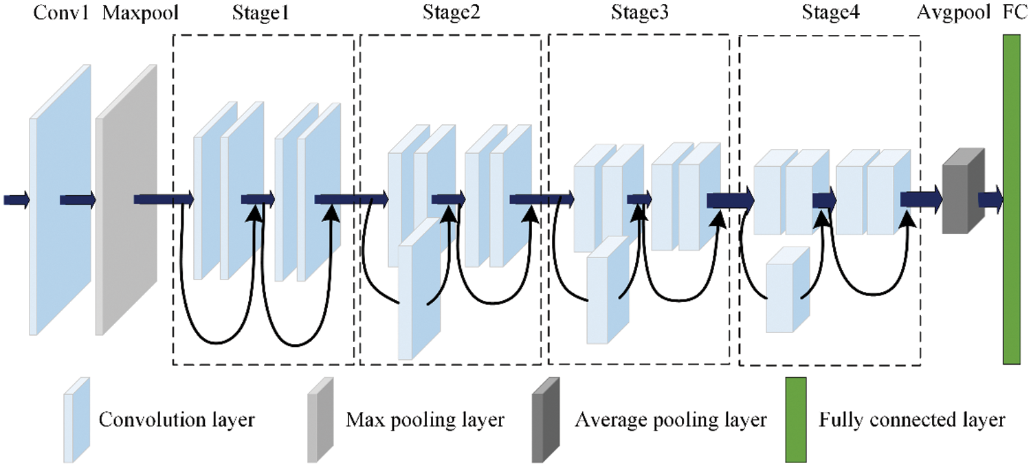
Figure 1: Structure of ResNet18
Starting from Stage2 of ResNet18, after each stage, the size of the feature map is reduced to half of the original size, and the number of channels is doubled. After 4 stages, the feature map with the shape of 7 × 7 × 512 is transferred to the final Avgpool and FC. The specific network architecture and internal parameters are shown in Table 1.

Due to the single size of the receptive field and the insufficient ability to shield interference information, it is difficult for ResNet18 to complete the task of identifying apple diseases in a complex environment. The purpose of this paper is to improve the application ability of the model in the production environment. From the perspectives of portability, economy, and practicality, embedded devices or mobile devices are more suitable for agricultural disease identification than high-performance computers and servers [31]. ResNet18 relies on a large number of parameters and layers to improve the learning ability of the network, which limits the deployment and operation of the model on resource-constrained devices [32]. Therefore, ResNet18 is not suitable for deployment on apple leaf disease identification equipment in the field.
The aim involves the characteristics of apple diseases in natural scenarios and the application requirements of limited storage space and computing resources of mobile devices. Based on ResNet18, the LW-ResNet model is constructed, and the structure is shown in Fig. 2.
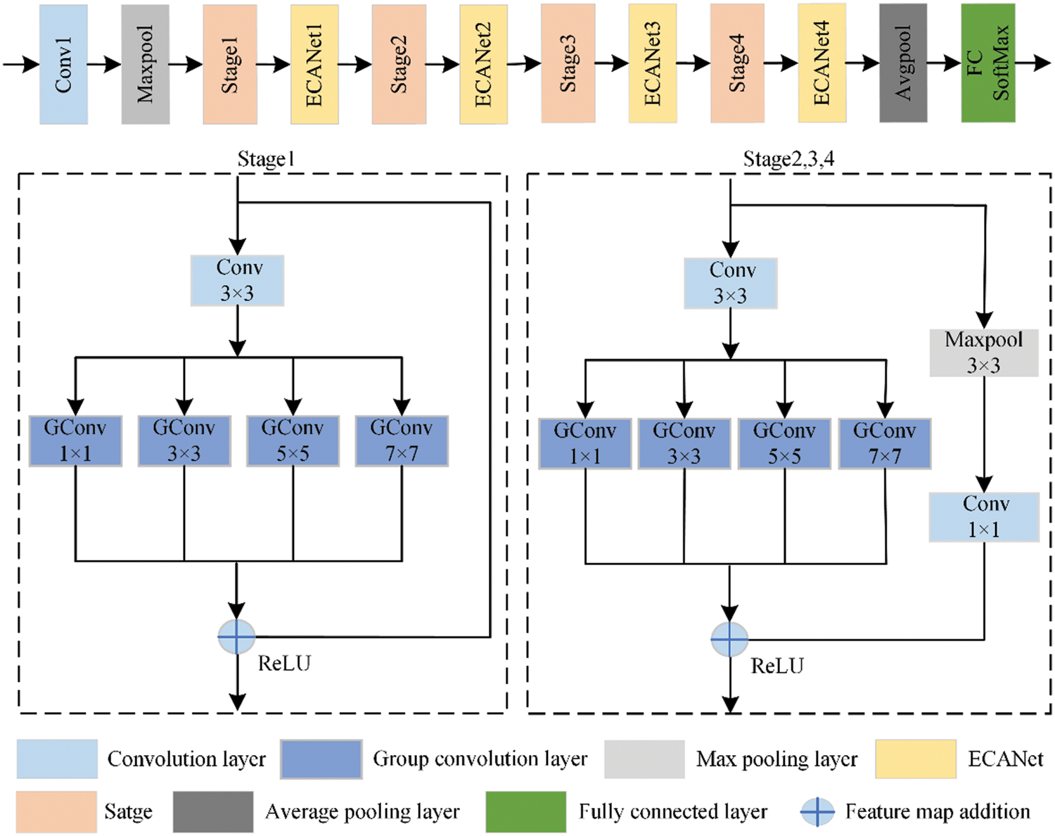
Figure 2: Structure of LW-ResNet
As shown in Table 2, the size change of the feature map of LW-ResNet is the same as that of the original model ResNet18, and the output channel of the fully connected layer of LW-ResNet is 7.

Only one residual module is retained in each stage of the network, and multiple receptive field sizes are added to the residual module, which reduces the number of model parameters and calculations and obtains a variety of local features. In this paper, the pooling layer and the convolutional layer are connected in series for identity mapping, which reduces the loss of information and strengthens the expression of the details of the lesions. A lightweight and efficient attention module (ECANet) is introduced between the residual modules to suppress the propagation of the environmental noise generated by the complex background during the model learning process.
3.2.2 Multiple Receptive Field Sizes
One of the difficulties in apple disease identification is that the sizes of the lesions are different, especially the small lesions. Because the richness of the detailed features of lesions is basically proportional to the number of pixels occupied, it is difficult to extract the features of small lesions, which leads to a decrease in the overall recognition accuracy of the model. For ResNet18, there are only convolutional layers with a size of 3 × 3 in the residual module. The receptive field of a single-scale convolution kernel is fixed, and the extracted features are limited, which cannot meet the feature information required to identify lesions of different sizes, especially small lesions, and it is necessary to combine features of multiple scales for judgment. Using traditional convolution kernels to obtain multi-scale features also leads to a significant increase in network parameter requirements, which increases the difficulty of model training and deployment. Therefore, this paper chooses the group convolution with lower parameters and complexity to construct a multi-scale feature extraction layer. The second layer of convolution in the residual module of ResNet18 is replaced with four different scale (1 × 1, 3 × 3, 5 × 5, 7 × 7) group convolutions to extract features of different scales.
The group convolution is shown in Fig. 3. The group convolution with a convolution kernel size of K × K divides the feature map of size H × W × M into G groups, the number of input channels in each group is M/G, the number of output channels in each group is N/G, and the total number of convolution kernels is N.
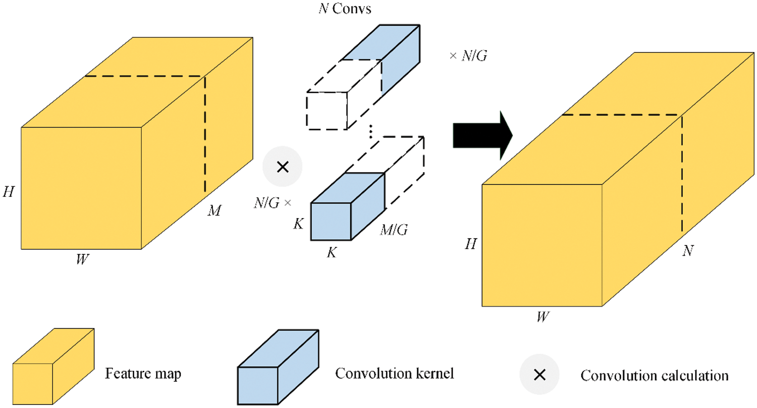
Figure 3: Group convolution
It can be seen from Eqs. (2) and (3) that the Parameters and FLOPs of the group convolution are only 1/G of the standard convolution.
Taking the residual module in Satge1 of LW-ResNet as an example, the input channel of each convolution (1 × 1, 3 × 3, 5 × 5, 7 × 7) in the multi-scale feature extraction layer is 16, the output channel is 16, and the size of the input and output feature maps is 56 × 56.
The number of parameters of the multi-scale feature extraction layer constructed by traditional convolution is 12 × 16 × 16 + 32 × 16 × 16 + 52 × 16 × 16 + 72 × 16 × 16 = 21504. The number of multi-scale feature extraction layer parameters constructed by group convolution with 16 groups (G = 16) is 12 × 16 × 16 × 1/16 + 32 × 16 × 16 × 1/16 + 52 × 16 × 16 × 1/16 + 72 × 16 × 16 × 1/16 = 1344, which reduces the number of parameters by 93.75% compared with the multi-scale feature extraction layer constructed by traditional convolution. Similarly, from Eq. (3), the FLOPs of the multi-scale feature extraction layer constructed by traditional convolution can be calculated to be 6.74E+07, and the FLOPs of the multi-scale feature extraction layer constructed by group convolution are 4.21E+06.
The Stage2, Satge3 and Stage4 modules in the original residual network are carried out by a convolution layer with a step size of 2 and convolution kernel size of 1 × 1 for channel elevation and feature graph size reduction to ensure feature matrix summative calculation and realize identity mapping. However, the step size is larger than the size of the convolution kernel, and useful features are missed when performing convolution calculations. At the same time, the average pooling layer emphasizes the down-sampling of the overall information features in the pooling area, ignoring the prominent color and texture features of the lesions, and retaining more useless background features, which is not conducive to the extraction of key features in the apple disease data. The max pooling layer outputs the maximum value in the entire pooling area, which can better retain the local details of the lesions and improve the generalization ability of the model. According to the characteristics of the apple disease image, a max pooling layer reduction feature size map with a step size of 2 and a size of 3 × 3 was selected, followed by a convolutional layer dimension raising channel with a step size of 1 and a convolution kernel size of 1 × 1 to compensate for the information loss caused by the original structure while maintaining the same number of parameters.
Since the data used in this paper are data on apple leaf diseases in a field environment, the background is complex and there are many environmental interference factors. There will be considerable noise in the model recognition process, which will be transmitted in the model learning process. As the number of network layers increases, the weight of the noise information in the feature map will also increase, which will eventually have a certain negative impact on the model. The channel attention mechanism weakens the channels that represent background features and reduces their weight [33], thereby reducing the negative impact of noise and other interference factors on the model recognition task. Most channel attention modules cannot consider low complexity and high performance at the same time [34]. For example, two fully connected layers are used by the classic SENet [35] module to exchange information between channels and reduce the dimensionality of features. The use of the fully connected layer makes SENet not lightweight, and the dimensionality reduction operation makes the channel and its predicted weight have no direct relationship, which has an impact on the overall performance of SENet.
One-dimensional convolution is used by ECANet [36] to combine neighbor channels to obtain weighted lesion features, to compensate for the defects caused by feature dimensionality reduction, to achieve local cross-channel interaction, and to better enhance the features of lesion areas. In addition, ECANet has a low parameter amount and complexity, and will not increase the storage overhead and calculation overhead of the network model too much. ECANet is suitable to be introduced into a lightweight network structure to improve the model's ability to focus on effective features in a complex environment, and to maintain the model's lightweight and fast characteristics. Therefore, we place the low-complexity and high-efficiency ECANet after each residual module. By recalibrating the channel characteristics generated by the residual module, the expression ability of the model is improved, and the goal of improving the recognition performance of the model is finally achieved.
The structure of ECANet is shown in Fig. 4, where W is the width of the feature map, H is the height of the feature map, C is the number of channels, U represents the original feature, and GAP represents the global average pooling operation. K represents not only the size of the one-dimensional convolution kernel but also the frequency of local cross-channel interaction, and Ũ is the weighted feature.
ECANet first uses global average pooling to aggregate the spatial information of each channel of the input feature U ∈ RW×H×C. The global average pooling operation is shown in Eq. (4).
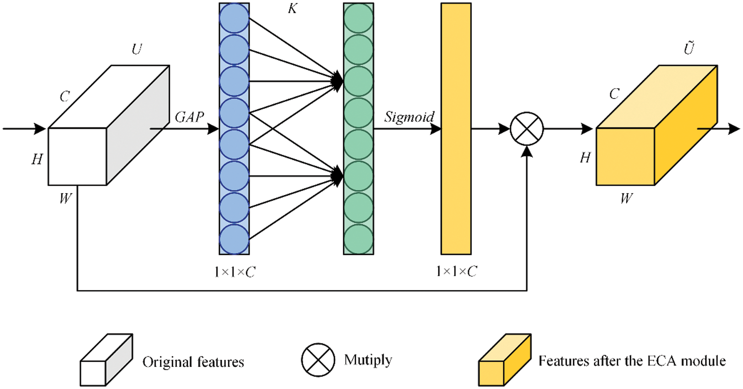
Figure 4: Structure of ECANet
Then, a one-dimensional convolution with a convolution kernel size of K is used to perform convolution calculation on GAP(U) to quickly extract the feature relationships of local K channels. The sigmoid function is used to calculate the activation value of the one-dimensional convolution output and obtain the weight ω ∈ R1×1×C, which represents the local relationship and importance of the feature channel. Sigmoid and ω are shown in Eqs. (5) and (6), where C1D represents a one-dimensional convolution.
Finally, to re-encode each channel feature of U, ω and U are multiplied element by element to obtain the feature map channel set Ũ. The important channel features are assigned large weights to achieve enhancement, while the invalid channel features are assigned small weights to achieve autonomous suppression.
In this chapter, the collected apple leaf images are used as research data, and ablation experiments and comparison experiments of different models are carried out under the same parameters to verify the effectiveness of the improved steps and the proposed model. Finally, the robustness of LW-ResNet is analyzed.
In this paper, images of 6 types of diseased leaves (alternaria leaf spot, powdery mildew, rust, scab, mosaic, anthracnose leaf blight) and healthy leaves of apples are taken as the research objects. The data are taken from the Kaggle competition dataset (https://www.kaggle.com/) and images publicly shared on the internet. The samples in the dataset are all complex background leaf disease images taken in the actual production environment, as shown in Fig. 5.
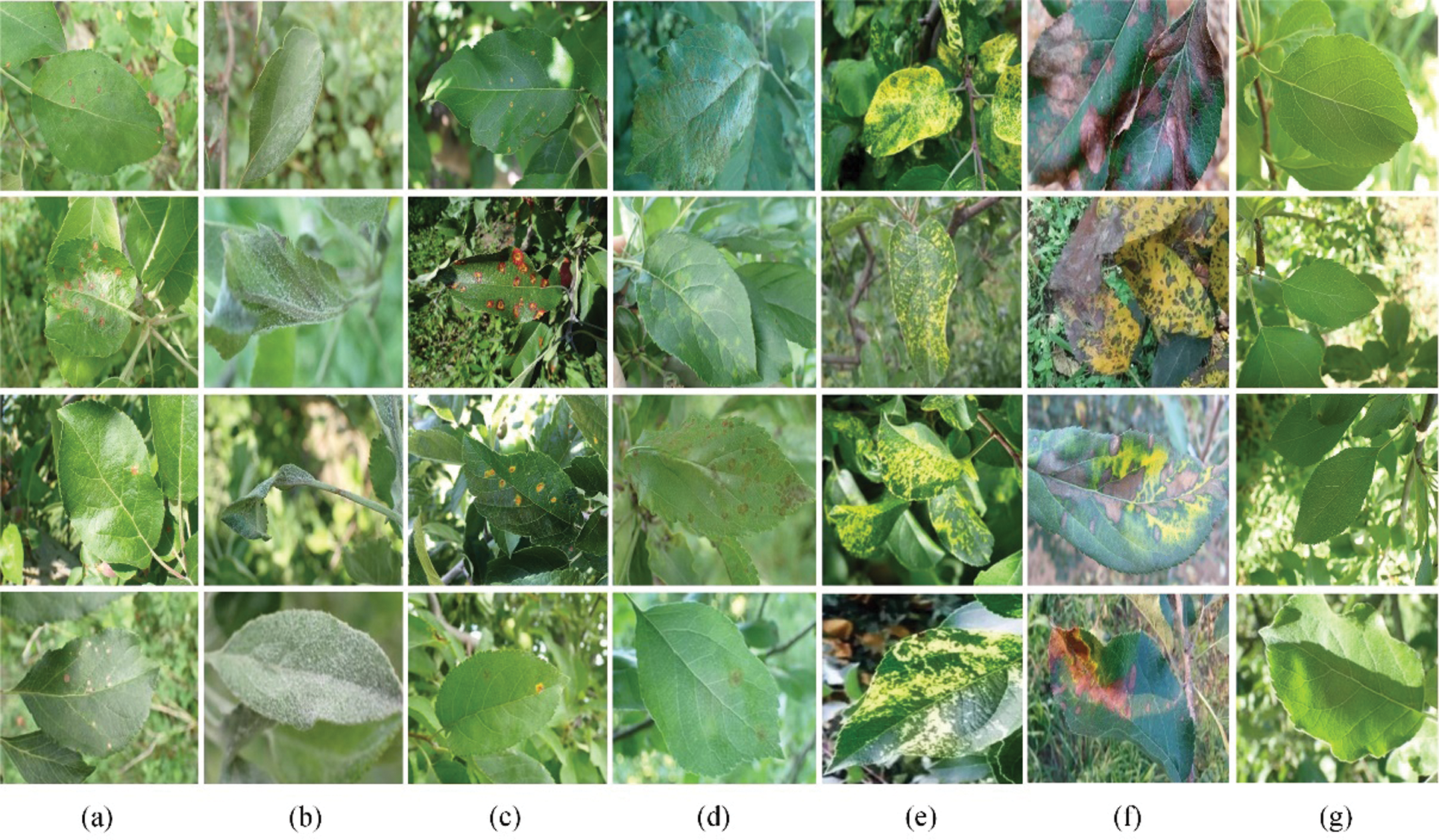
Figure 5: Examples of dataset: (a) Alternaria leaf spot, (b) Powdery mildew, (c) Rust, (d) Scab, (e) Mosaic, (f) Anthracnose leaf blight, (g) Healthy
The data distribution is shown in Fig. 6, where 0 is alternaria leaf spot, 1 is powdery mildew, 2 is rust, 3 is scab, 4 is mosaic, 5 is anthracnose leaf blight, and 6 is healthy leaves.
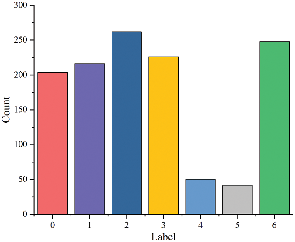
Figure 6: Data distribution and label
It can be seen from Fig. 6 that the total number of samples in the dataset is insufficient and the distribution of various samples is unbalanced, which will affect the recognition effect of the model [37–39]. Therefore, this paper uses random rotation, random brightness contrast enhancement, random Gaussian noise and other data enhancement methods to expand the data.
Fig. 7 shows some samples of enhanced images. Taking the apple mosaic image as an example, 50 original images are enhanced to 200 by random rotation, and then the images are expanded from 200 to 1200 by brightness enhancement, contrast enhancement and Gaussian noise enhancement.
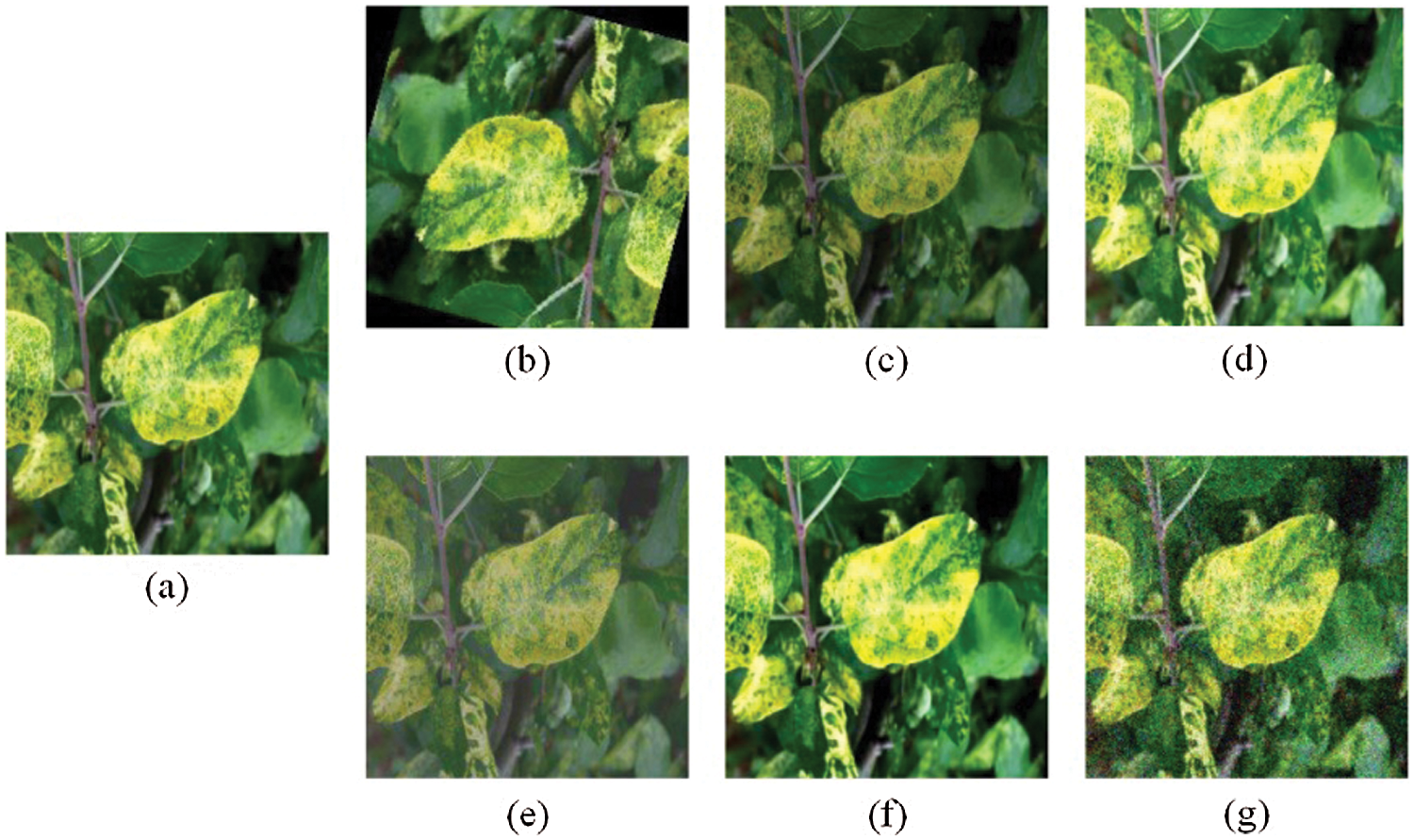
Figure 7: Examples of data enhancement: (a) Original, (b) Rotation, (c) Low brightness, (d) High brightness, (e) Low contrast, (f) High contrast, (g) Gaussian noise
As shown in Table 3, the number of expanded images is basically balanced, with a total of 9,480. Eighty percent of the dataset was randomly selected as the training set, and 20% was selected as the test set. This paper uses 5-fold cross-validation. Each fold, 6077 images are extracted from the training set for training, and 1519 images are used for verification.

The apple disease recognition model was constructed by the deep learning framework PyTorch. All experiments were carried out in the Window 10 environment. The CPU is an Intel(R) Xeon(R) W-2245, and the GPU is an NVIDIA Quadro RTX graphics card with 16 GB memory.
The adaptive moment estimation algorithm (Adam) [40] is efficient and has low memory requirements, so it was selected as the parameter optimizer for this experiment. To train the best model, we use the original model ResNet18 to conduct a series of pre-experiments on the dataset. The learning rate is set to 4 groups, 0.0001, 0.001, 0.01, and 0.1, and the batch-size is set to 16, 32, 64, and 128. Through comparative experiments, the learning rate and batch-size are finally determined to be 0.001 and 32, respectively. In the pre-experiment process, we found that ResNet18 had converged when it was less than 50 epochs, so we set the epoch of the subsequent experiments to 50. The parameter settings are shown in Table 4.

The precision, recall, and F1-score are used by us to comprehensively evaluate the recognition performance of the model. Cost and efficiency are important criteria to measure the practicability of a model or algorithm and are considered by many researchers [41,42]. Parameter memory requirements and FLOPs are used by us to evaluate the storage cost and calculation cost of the model, and FPS and running time are used by us to evaluate the time cost of the model.
Precision (Per) and recall (Rec) are shown in Eqs. (7) and (8). TP represents the number of positive samples predicted to be positive; TN is the number of negative samples predicted to be negative; FP is the number of negative samples predicted to be positive; and FN represents the number of positive samples predicted to be negative. F1-score (F1) is shown in Eq. (9), and its value range is [0, 1]. The higher the value is, the better the recognition performance of the model.
The parameter memory requirement is determined by the number of parameters. Under the premise of meeting the task requirements, the smaller the parameter memory is, the lower the hardware requirements of the model and the higher the applicability.
FLOPs are used to measure the number of operations of the model, which refers to the number of floating-point operations performed by the model for complete forward propagation after a single sample is input, that is, the time complexity of the model. The lower the FLOPs, the less calculation required for the model and the shorter the network execution time.
FPS is the number of images that can be processed per second and is used to measure the recognition speed of the model. The larger the FPS is, the faster the model recognition speed.
The running time represents the time from when the model is trained to the completion of the training. The shorter the running time is, the faster the model training speed.
4.4.1 Comparative Analysis of Different Ablation Schemes
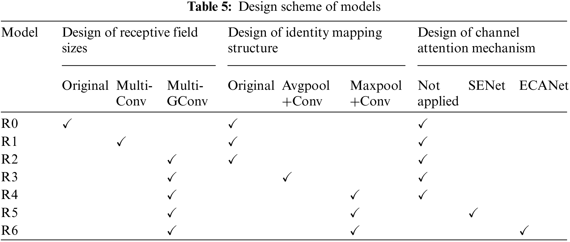
The design scheme of the ablation experiment is shown in Table 5. The design of the receptive field includes three types: the original receptive field, the multi-scale receptive field composed of ordinary convolution (Multi-Conv), and the multi-scale receptive field composed of group convolution (Multi-GConv). The structure of identity mapping is designed as an original structure, an identity mapping structure composed of an average pooling layer and a convolutional layer (Avgpool+Conv), and an identity mapping structure composed of a max pooling layer and a convolutional layer (Maxpool+Conv). The attention mechanism is designed into three types: no mechanism is applied, SENet [35] is used, and ECANet [36] is used.
The experimental results of each scheme on the test set are shown in Table 6. By comparing R0, R1 and R2, it can be seen that the features extracted by the model after introducing multi-scale receptive fields can more accurately characterize different diseases. R2 uses group convolution to construct a multi-scale feature extraction layer, which greatly improves FPS. Because each convolution kernel in the group convolution calculates only a part of the input channel, there is a lack of information exchange between each group of channels, which leads to a slight decrease in the generalization ability of the model. Compared with R1, the average precision, recall, and F1-score of R2 decreased by 0.16%, 0.26%, and 0.14%, respectively. It can be seen from R3 and R4 that the identity mapping structure of the max pooling layer is better than that of the average pooling layer, and its average precision, recall, and F1-score are higher by 0.31%, 0.42%, and 0.41%, respectively. It shows that the max pooling layer can better highlight the feature points of the lesions in the feature map that are significantly different from the surrounding pixels, and improve the overall recognition performance of the model.

R5 and R6 use SENet and ECANet, respectively. From the experimental results in Table 6 and the curves in Figs. 8 and 9, it can be seen that the use of the attention mechanism can help improve model recognition performance and accelerate model convergence, but they sacrifice image recognition time and running time to varying degrees. Compared with SENet, ECANet improves the accuracy of model recognition more notably and reduces the FPS and running time of the model to a lesser extent. Since ECANet discards the fully connected layer in SENet and chooses to use a one-dimensional convolution for the convolution operation and fusion of local channel information, the use of ECANet hardly affects the number of model parameters and time complexity. ECANet's light weight and high efficiency are fully embodied.
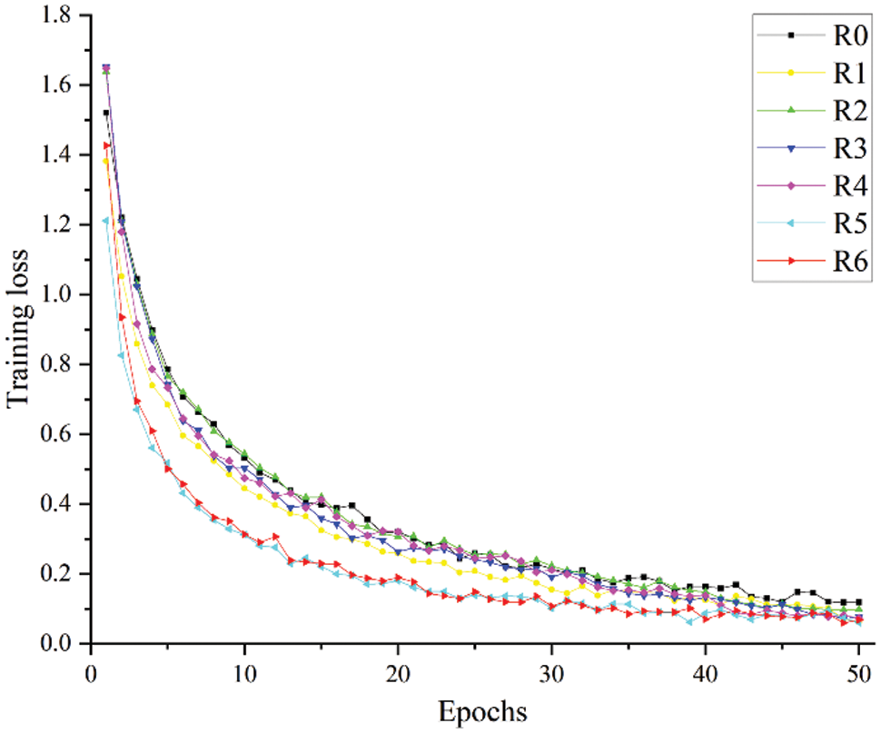
Figure 8: Training loss of different experimental schemes
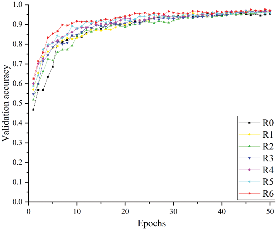
Figure 9: Verification accuracy of different experimental schemes
The heatmap shows the contribution degree of different areas in the original image to the output category of the model. Fig. 10 is an example of the heatmap of each experimental scheme. The redder the color is, the higher the model's attention to the area.
The overall recognition performance of R1--R5 combined with the optimization step is improved compared to R0. However, it can be seen from Figs. 10c and 10d that in some types of sample data, the use of multi-scale feature extraction layers makes the model pay more attention to redundant information in the background. The main reason is that the construction of a multi-scale feature extraction layer improves the model's ability to extract lesions and improves the ability to capture background features. As shown in Fig. 10f, the max pooling layer can solve the problem of the deviation of the estimated mean caused by the parameter error of the convolutional layer and highlight the features of lesions that are useful for the recognition task. Since the edges of branches and trunks, the edges of other leaves, and high-brightness light spots all have larger element values in local areas, they are easily retained by the max pooling layer and passed down. The model adopting the improved identity mapping structure's attention to lesion features is also affected by a certain degree of background interference. As shown in Fig. 10g, the model introduced with ECANet can effectively suppress most noises and reduce the background interference caused by the multi-scale feature extraction layer and the improved identity mapping structure to the recognition task. However, individual noise points that are extremely similar to lesion features are strengthened. The main reason is that during the feature extraction process of the network model, disease spots, other leaves, branches, light spots, soil, etc., in the image contribute differently to disease recognition, and different weights should be assigned. The ECANet module models the dependency between the channels of the feature map so that different positions of the same feature map have the same channel weight information. When the feature strength of the target information is weak, weakly related information with strong feature strength will attract the attention of the model. As a result, the background in the image of label 0 is increased attention.
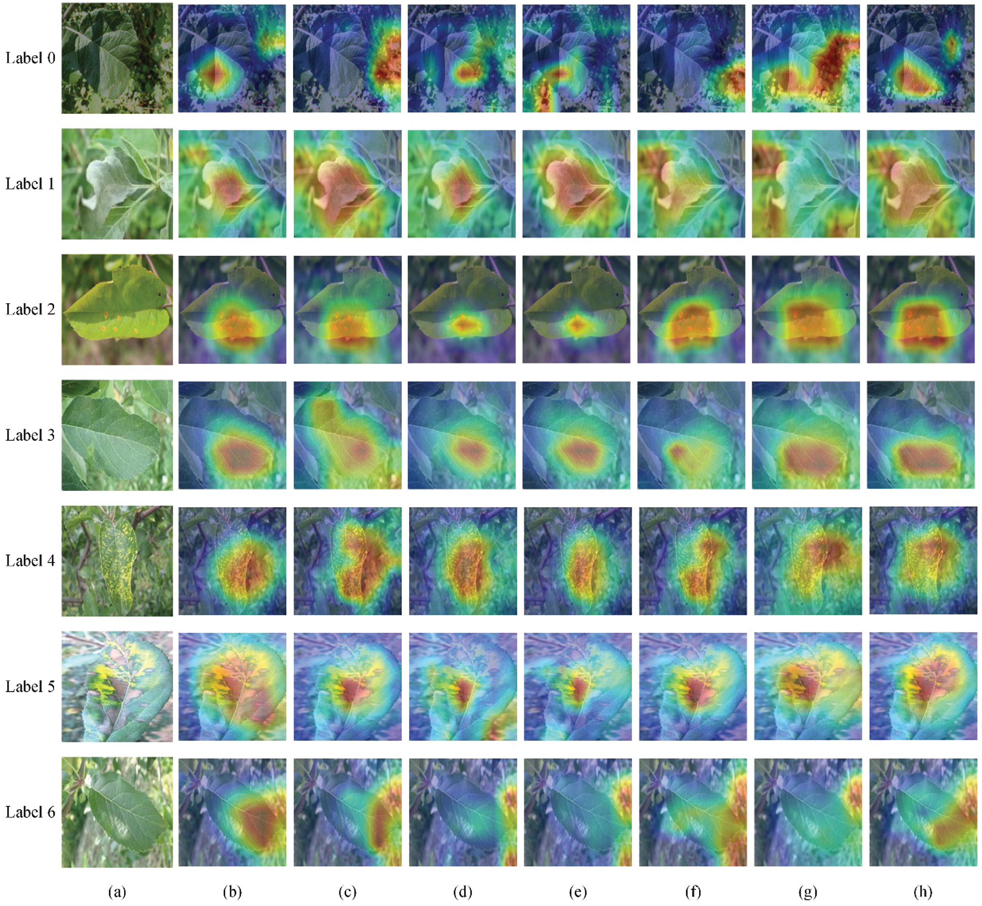
Figure 10: Examples of heatmaps of different experimental schemes: (a) Original images, (b) Heatmaps of R0, (c) Heatmaps of R1, (d) Heatmaps of R2, (e) Heatmaps of R3, (f) Heatmaps of R4, (g) Heatmaps of R5, (h) Heatmaps of R6
In general, the R6 model, which combines the multi-scale feature extraction layer, improves the identity mapping structure, introduces the ECANet module, and pays more attention to the lesion area than the R0--R5 models.
4.4.2 Comparative Analysis of Different Models
To evaluate the performance of the proposed recognition model, we compared the LW-ResNet model with some representative convolutional neural networks under the same parameter settings, including ResNet18 [27], VGG16 [43], DenseNet121 [44], SqueezeNet [45], MobileNetV2 [46], ShuffleNetV2 [47] and GhostNet [48]. The experimental results are shown in Table 7.

As shown in Table 7, the average accuracy, recall and F1-score of the proposed model reach 97.81%, 97.86% and 97.83%, respectively, which are better than the performances of the control network. The parameter memory of LW-ResNet is 2.32 MB, which is 17%--52% smaller than the two lightweight networks SqueezeNet and ShuffleNetV2 with the smallest parameter memory in the control network. Among the eight models, LW-ResNet has the highest image processing speed and the least running time. However, the complexity of LW-ResNet still needs to be reduced. The FLOPs of LW-ResNet are 7.3E+07 higher than those of ShuffleNetV2. The improved model proposed in this paper has high recognition accuracy and speed, low parameter memory and acceptable complexity. The proposed model has strong practicability and is suitable for embedding on a portable device chip with limited resources.
Fig. 11 shows the precision of the 8 models on the images of each category in the dataset. To better observe the recognition effect of the 8 models on various images, we draw columns of different colors according to the different intervals of precision. If the precision is above 96.25%, the column is drawn in red; when the precision is in the range of 92.5%--96.25%, the column is drawn in orange; when the precision is in the range of 88.75%--92.5%, the column is drawn in yellow. By analogy, as the precision decreases, the color of the column appears green, light blue, and dark blue. The drawing method of Figs. 12 and 13 is similar to that of Fig. 11.
It can be seen from Figs. 11–13 that the precision, recall and F1-score of ResNet18, which is used as the basic network of this paper, can be maintained above 88% on 7 categories of images. DenseNet121 has a poor recognition effect on alternaria leaf spot and scab. VGG16 and SqueezeNet are unsatisfactory in the recognition of most categories of images. MobileNetV2, ShuffleNetV2 and GhostNet perform similarly. They generally have better recognition results on rust images, mosaic images, anthracnose leaf blight images, and healthy leaf images, but their F1-score on alternaria leaf spot images and scab images can only reach more than 85%. LW-ResNet has a relatively balanced recognition effect for each category of images, and the precision, recall, and F1-score of each category of images can be maintained above 92.5%. This balance shows that the LW-ResNet model is effective in the identification tasks of these 6 common diseased leaves and healthy leaves.
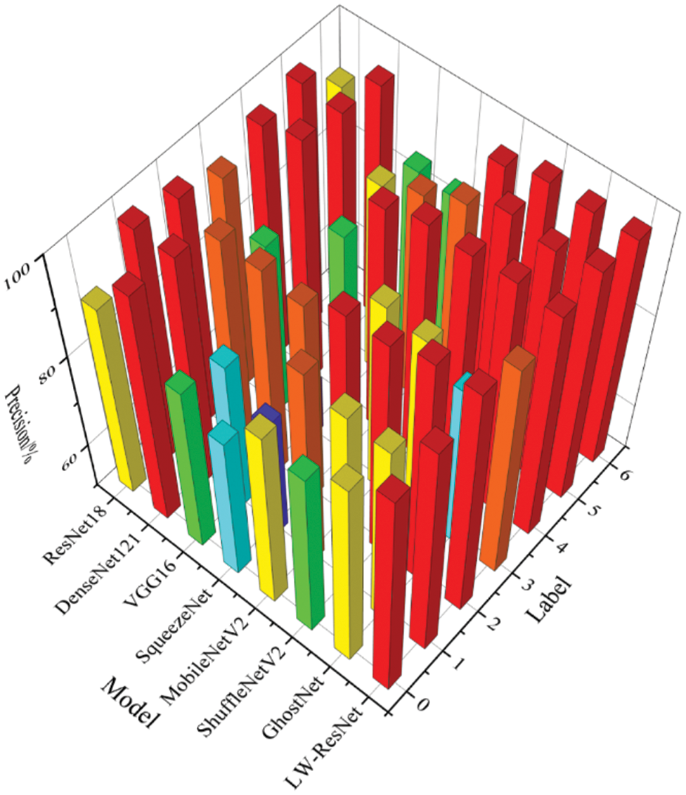
Figure 11: Precision of different models on each category of images
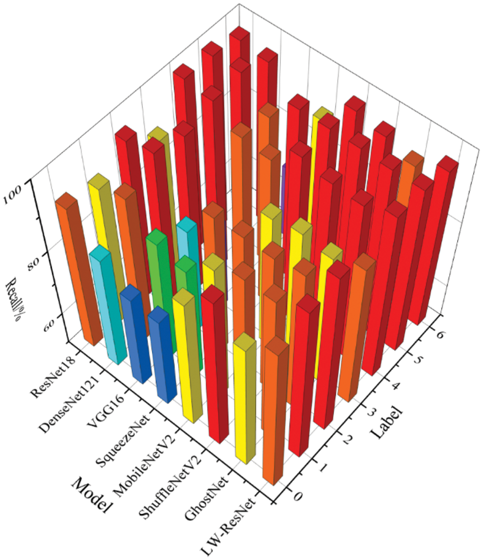
Figure 12: Recall of different models on each category of images
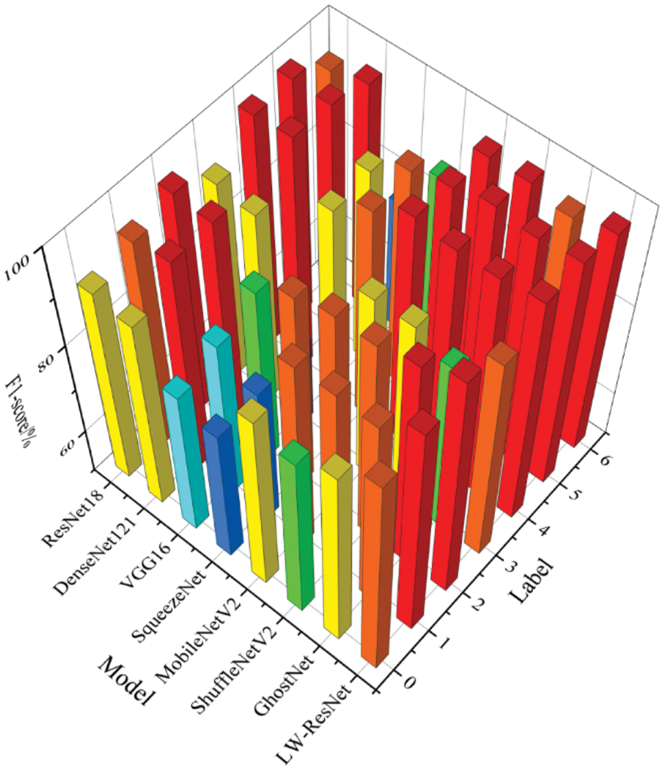
Figure 13: F1-score of different models on each category of images
Fig. 14 shows the relationship curve between the training loss and epoch for the 8 models. It can be clearly seen that as the number of epochs increases, the training loss of each model tends to be stable, and there is no major fluctuation. Among them, the convergence speed of the LW-ResNet model is significantly better than that of the other models. After the 12th epoch, the loss of the proposed model remained below 0.15, while ResNet18, DenseNet121, ShuffleNetV2 and GhostNet remained below 0.15 after the 43rd, 34th, 44th and 47th epochs, respectively. From the perspective of loss convergence, the LW-ResNet model has the best training effect.
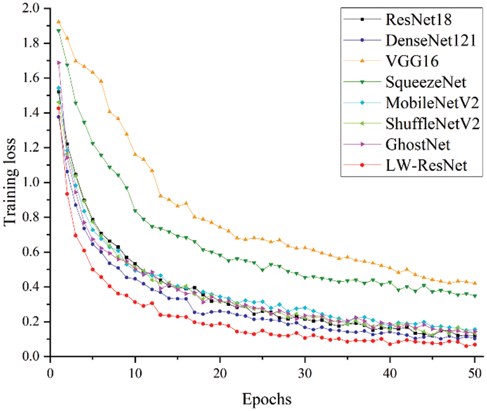
Figure 14: Relationship between training loss and epochs
The relationship between the verification accuracy and epoch for each model is shown in Fig. 15. The accuracy of the LW-ResNet model reached 83% in the 4th epoch, and the accuracy stabilized above 90% after 9 epochs, while other models reached 84% only in the 9th epoch. Obviously, it can be seen that the LW-ResNet model has a fast convergence speed and high accuracy.
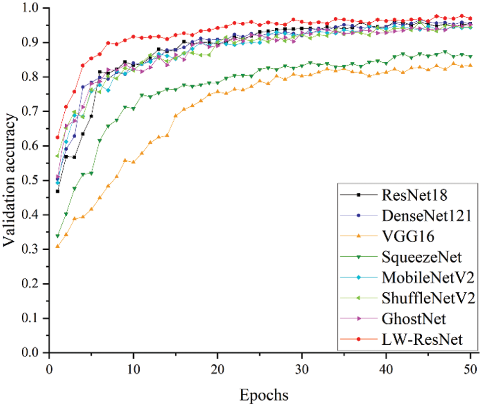
Figure 15: Relationship between validation accuracy and epochs
As shown in Table 8, to verify the practicability of the proposed model in apple disease recognition tasks, our model is compared with other apple disease recognition models proposed by other studies.
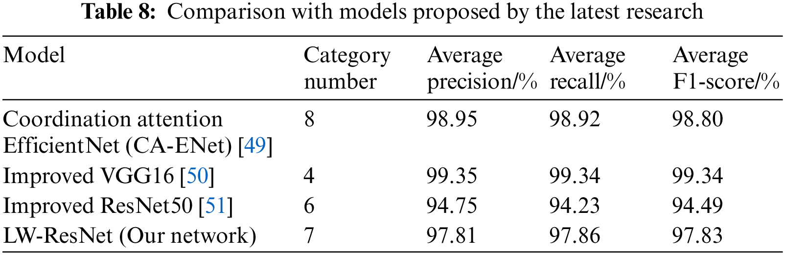
Coordination attention EfficientNet (CA-ENet) was proposed by Peng et al. [49]. They used part of PlantVillage data combined with self-built image samples as experimental data to conduct a study on the identification of eight types of apple leaves (7 types of diseased leaves and healthy leaves). The average precision, recall, and F1-score are 98.95%, 98.92%, and 98.80%, respectively, and the recognition results are all higher than those of model proposed in this paper. However, the parameter memory of CA-ENet is 21 MB, which is approximately 10 times that of the model in this paper. It is obvious that the model proposed in this article is easier to deploy and install.
VGG16 was improved by Qian et al. [50]. The global average pooling layer was used to replace the fully connected layer in the original model. The number of parameters of the improved model was only 11% of the original model VGG16, and the average F1-score was 99.34%. Although they have achieved good results in model parameter compression and improvement of recognition effect, the basic network they chose is too large, so that the network parameter memory after substantial compression is still much higher than that of the LW-ResNet model in this paper. Their experimental data are a single background apple disease image, and the model has difficulty maintaining high recognition accuracy in the real environment.
Part of the data used by Yan et al. [51] is also taken from the Kaggle competition platform, so the improved ResNet50 is highly comparable to our LW-ResNet. They changed the information circulation method of the network and introduced pyramid convolution and expansion convolution so that the improved ResNet50 has strong anti-noise ability and robustness. The average precision, recall, and F1-score of the improved ResNet50 are 3.06%, 3.63%, and 3.34% lower than those of our LW-ResNet, and its parameter memory is 93.51 MB higher than that of LW-ResNet, which further explains the proposed LW-ResNet has better practicability in this paper.
4.4.3 Analysis of LW-ResNet Robustness on Apple Leaf Dataset
Fig. 16 shows the confusion matrix results of the LW-ResNet model on the test set. From the confusion matrix, it can be seen that the images of rust, mosaic disease and anthracnose leaf blight are easy to recognize, among which 311 of 312 images of rust are correctly classified, 240 images of mosaic disease are correctly identified, and only 1 of 268 images of anthracnose leaf blight is incorrectly identified. Scab and healthy leaves are prone to misclassification, and scab is mistakenly classified as alternaria leaf spot frequently. Through the analysis of the dataset of this paper, it is found that the differences among the same type of diseases is large, and the small differences among the different types of diseases are the main reason for the misclassification of the images.
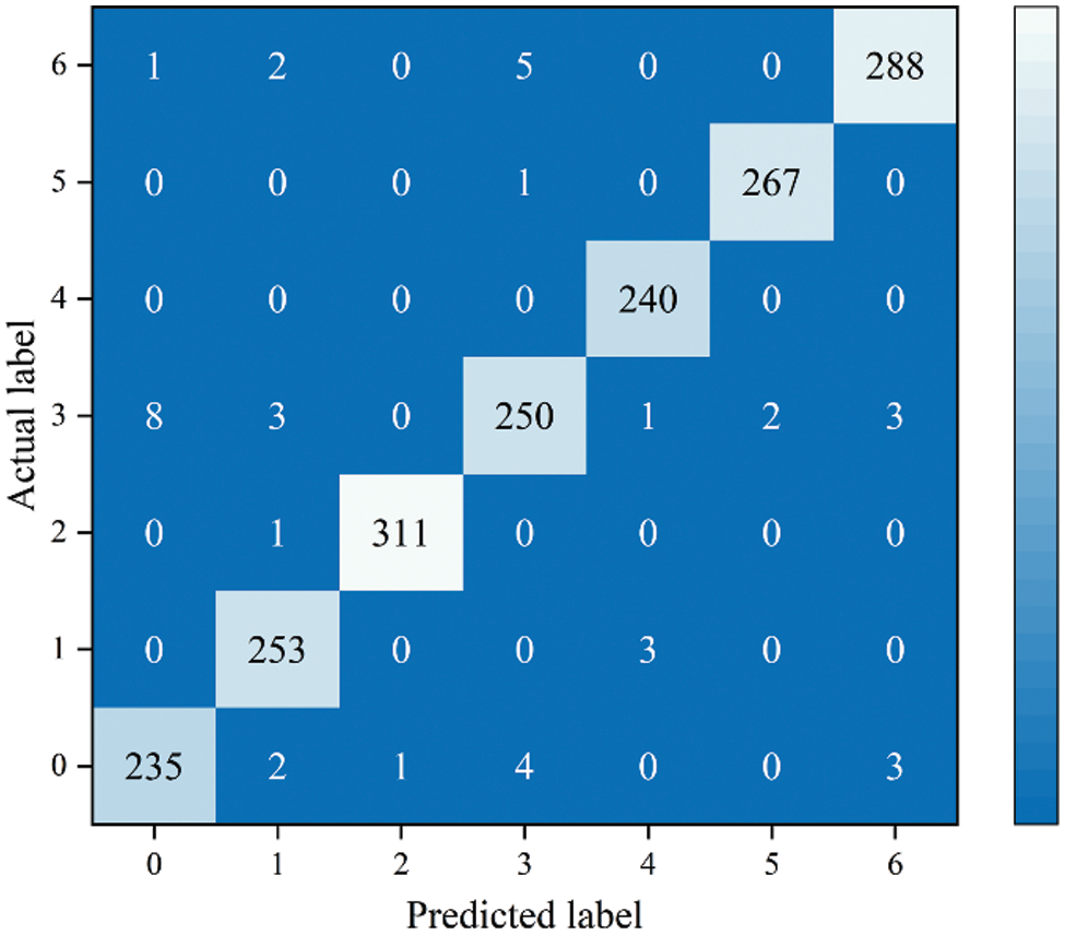
Figure 16: Confusion matrix of LW-ResNet on the test set
As shown in Fig. 17, the scab spots in the early stage of the disease are light yellow round or radial. The diseased leaves are very similar to healthy leaves, and it is difficult to correctly classify them even manually.
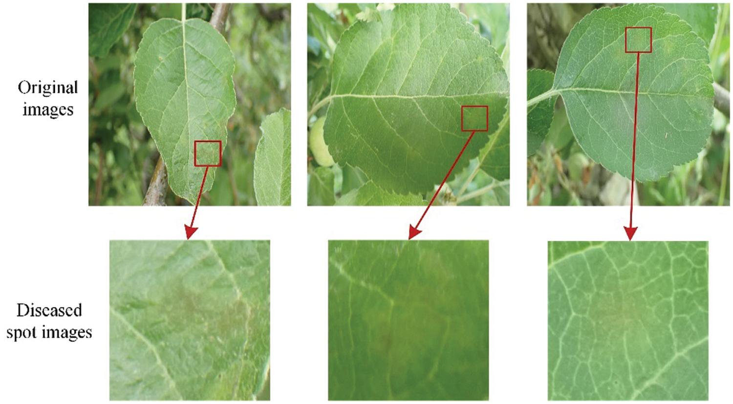
Figure 17: Examples of early stage of scab
As shown in Fig. 18, the late stages of scab turn dark brown, which are similar to those of alternaria leaf spot, so they are prone to misclassification.
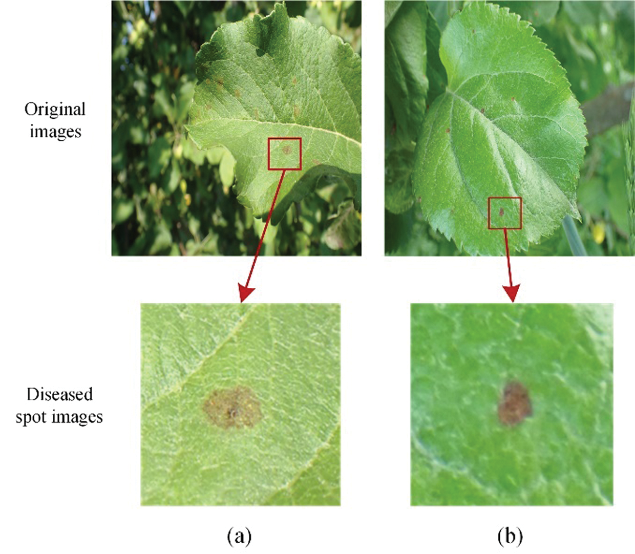
Figure 18: Examples of alternaria leaf spot and late stage of scab: (a) Late stage of scab, (b) Alternaria leaf spot
In general, the average accuracy of LW-ResNet on the test set is 97.88%, and the precision, recall, and F1-score of each category of images also reach more than 92.5%. These values shows that the LW-ResNet model has high robustness and strong recognition performance.
In this work, we propose a lightweight and efficient model for apple leaf disease identification. We establish a dataset of apple leaf diseases with a complex background, and enhance the data to improve the generalization ability of the model [52]. According to the images of disease spots of different sizes and the complex background, this paper designs a lightweight LW-ResNet model. The proposed model has high recognition accuracy, few parameters, fast recognition speed, and high practicability and robustness.
From the ablation experimental results, the improvement steps designed in this paper can improve the recognition accuracy and speed of the model, and reduce the number of parameters and complexity of the model, but there are still problems. Using group convolution to build a multi-scale feature extraction layer can compress the model to a large extent and improve the recognition speed of the model. However, group convolution also hinders the flow of information between feature channels. This hindrance is consistent with the conclusions of studies [53]. We add a maximum pooling layer to the identity mapping structure to better retain the edge and texture characteristics of the lesions, and at the same time, the irrelevant information with greater feature strength in the image is directly transferred from the shallow layer of the network to the deep layer. In addition, we use an efficient channel attention mechanism to reduce the impact of complex background on the model recognition effect from the channel point of view, ignoring the spatial information, resulting in some noise points with large pixel values interfering with the model's extraction of lesion features, which is consistent with the conclusions of study [54]. It can be seen from the example of the heatmap that the influence of the complex background still exists, and studies [55,56] have also proven that the complexity of the background will affect the recognition effect of the model.
Through the performance comparison of different models and the robustness analysis of the LW-ResNet model, it can be seen that the model proposed in this paper has a good balance of recognition accuracy, speed, model size and other indicators. The performance of the proposed model is better than that of the classic network model, and it has a better recognition effect for each type of diseased leaf sample, but the complexity of the model still has room to decrease. Through the confusion matrix of LW-ResNet, it can be found that the difference between the classes is small, and the difference within the class is still one of the main reasons for the images to be misclassified [57], which also reflects the importance of continuing to refine the dataset and improving the fine feature extraction ability of the model [58].
From the above discussion, the limitations of the LW-ResNet model can be summarized as follows: LW-ResNet has insufficient ability to distinguish high and low information features with different spatial locations and insufficient ability to extract fine-grained features. This paper aims to construct an efficient lightweight model suitable for real production links. It has become an important task to improve the recognition ability of the model under the background of high complexity and to construct a dataset of disease images with different stages of disease. In the future, the designed model can be optimized by advanced meta-heuristic algorithms [59–61] to be applied to other problems, such as transportation and logistics management [62], complex systems [63], signal processing [64], path planning [65,66], and controllable charging [67].
To improve the application ability of the model in the actual environment, this paper proposes a lightweight LW-ResNet model. The proposed model makes up for the shortcomings of many parameters, high complexity, and poor generalization ability in the real environment of ResNet18 and realizes the rapid identification of 6 kinds of diseased apple leaves and healthy leaves under a complex background. The average precision, recall, and F1-score of the method in this paper are all over 97%, the parameter memory is only 6% of the original model ResNet18, and FLOPs is reduced by 86%. In addition, LW-ResNet also has obvious advantages in recognition speed and training speed. It can process 276 images per second, and the training time is only 0.83 h. It is proposed that the model has strong robustness and is suitable for application in small embedded devices with limited resources. It can play a positive role in the prevention and control of apple leaf diseases in the agricultural production process.
However, there are still some problems with this method that urgently need to be solved. The future work is as follows:
(1) From experiments, it is found that the ability of the model in this paper to suppress background noise still needs to be improved. Future research will focus on improving the sensitivity of the model to the difference between the background and the target in the spatial domain.
(2) Differences in different disease stages and similar disease characteristics often affect the recognition performance of the model. In subsequent research, we will collect apple leaves with different stages of disease by shooting, expanding and refining the dataset and combine the dataset design for the apple disease recognition model with a strong ability to extract fine-grained features.
Funding Statement: This research was funded by the Science and Technology Development Program of Jilin Province (20190301024NY) and the Precision Agriculture and Big Data Engineering Research Center of Jilin Province (2020C005).
Conflicts of Interest: The authors declare that they have no conflicts of interest to report regarding the present study.
1. Jiang, H., Meng, X., Ma, J., Sun, X., Wang, Y. et al. (2021). Control effect of fungicide pyraclostrobin alternately applied with bordeaux mixture against apple glomerella leaf spot and its residue after preharvest application in China. Crop Protection, 142(5), 105489. DOI 10.1016/j.cropro.2020.105489. [Google Scholar] [CrossRef]
2. Kour, V. P., Arora, S. (2019). Particle swarm optimization based support vector machine (P-SVM) for the segmentation and classification of plants. IEEE Access, 7, 29374–29385. DOI 10.1109/ACCESS.2019.2901900. [Google Scholar] [CrossRef]
3. Kaur, P., Pannu, H. S., Malhi, A. K. (2019). Plant disease recognition using fractional-order zernike moments and SVM classifier. Neural Computing and Applications, 31(12), 8749–8768. DOI 10.1007/s00521-018-3939-6. [Google Scholar] [CrossRef]
4. Abdulridha, J., Batuman, O., Ampatzidis, Y. (2019). UAV-based remote sensing technique to detect citrus canker disease utilizing hyperspectral imaging and machine learning. Remote Sensing, 11(11), 1373. DOI 10.3390/rs11111373. [Google Scholar] [CrossRef]
5. Wójtowicz, A., Piekarczyk, J., Czernecki, B., Ratajkiewicz, H. (2021). A random forest model for the classification of wheat and rye leaf rust symptoms based on pure spectra at leaf scale. Journal of Photochemistry and Photobiology B: Biology, 223, 112278. DOI 10.1016/j.jphotobiol.2021.112278. [Google Scholar] [CrossRef]
6. Gomez Selvaraj, M., Vergara, A., Montenegro, F., Alonso Ruiz, H., Safari, N. et al. (2020). Detection of banana plants and their major diseases through aerial images and machine learning methods: A case study in DR Congo and republic of Benin. ISPRS Journal of Photogrammetry and Remote Sensing, 169, 110–124. DOI 10.1016/j.isprsjprs.2020.08.025. [Google Scholar] [CrossRef]
7. Hu, G., Yin, C., Wan, M., Zhang, Y., Fang, Y. (2020). Recognition of diseased pinus trees in UAV images using deep learning and AdaBoost classifier. Biosystems Engineering, 194, 138–151. DOI 10.1016/j.biosystemseng.2020.03.021. [Google Scholar] [CrossRef]
8. Osco, L. P., Arruda, M. D. S. D., Marcato Junior, J., da Silva, N. B., Ramos, A. P. M. et al. (2020). A convolutional neural network approach for counting and geolocating citrus-trees in UAV multispectral imagery. ISPRS Journal of Photogrammetry and Remote Sensing, 160, 97–106. DOI 10.1016/j.isprsjprs.2019.12.010. [Google Scholar] [CrossRef]
9. Pi, W., Du, J., Bi, Y., Gao, X., Zhu, X. (2021). 3D-CNN based UAV hyperspectral imagery for grassland degradation indicator ground object classification research. Ecological Informatics, 62, 101278. DOI 10.1016/j.ecoinf.2021.101278. [Google Scholar] [CrossRef]
10. Jahanbakhshi, A., Momeny, M., Mahmoudi, M., Radeva, P. (2021). Waste management using an automatic sorting system for carrot fruit based on image processing technique and improved deep neural networks. Energy Reports, 7, 5248–5256. DOI 10.1016/j.egyr.2021.08.028. [Google Scholar] [CrossRef]
11. Karthik, R., Hariharan, M., Anand, S., Mathikshara, P., Johnson, A. et al. (2020). Attention embedded residual CNN for disease detection in tomato leaves. Applied Soft Computing, 86, 105933. DOI 10.1016/j.asoc.2019.105933. [Google Scholar] [CrossRef]
12. Liu, B., Ding, Z., Tian, L., He, D., Li, S. et al. (2020). Grape leaf disease identification using improved deep convolutional neural networks. Frontiers in Plant Science, 11, 1082. DOI 10.3389/fpls.2020.01082. [Google Scholar] [CrossRef]
13. Picon, A., Alvarez-Gila, A., Seitz, M., Ortiz-Barredo, A., Echazarra, J. et al. (2019). Deep convolutional neural networks for mobile capture device-based crop disease classification in the wild. Computers and Electronics in Agriculture, 161, 280–290. DOI 10.1016/j.compag.2018.04.002. [Google Scholar] [CrossRef]
14. Toseef, M., Khan, M. J. (2018). An intelligent mobile application for diagnosis of crop diseases in Pakistan using fuzzy inference system. Computers and Electronics in Agriculture, 153, 1–11. DOI 10.1016/j.compag.2018.07.034. [Google Scholar] [CrossRef]
15. de Vita, F., Nocera, G., Bruneo, D., Tomaselli, V., Giacalone, D. et al. (2021). Porting deep neural networks on the edge via dynamic K-means compression: A case study of plant disease detection. Pervasive and Mobile Computing, 75, 101437. DOI 10.1016/j.pmcj.2021.101437. [Google Scholar] [CrossRef]
16. Xia, M., Huang, Z., Tian, L., Wang, H., Chang, V. et al. (2021). Sparknoc: An energy-efficiency FPGA-based accelerator using optimized lightweight CNN for edge computing. Journal of Systems Architecture, 115(4), 101991. DOI 10.1016/j.sysarc.2021.101991. [Google Scholar] [CrossRef]
17. Liu, J., Wang, X. (2021). Plant diseases and pests detection based on deep learning: A review. Plant Methods, 17(1), 22. DOI 10.1186/s13007-021-00722-9. [Google Scholar] [CrossRef]
18. Wu, X., Sahoo, D., Hoi, S. C. H. (2020). Recent advances in deep learning for object detection. Neurocomputing, 396, 39–64. DOI 10.1016/j.neucom.2020.01.085. [Google Scholar] [CrossRef]
19. Tang, Z., Yang, J., Li, Z., Qi, F. (2020). Grape disease image classification based on lightweight convolution neural networks and channelwise attention. Computers and Electronics in Agriculture, 178(2), 105735. DOI 10.1016/j.compag.2020.105735. [Google Scholar] [CrossRef]
20. Yadav, S., Sengar, N., Singh, A., Singh, A., Dutta, M. K. (2021). Identification of disease using deep learning and evaluation of bacteriosis in peach leaf. Ecological Informatics, 61, 101247. DOI 10.1016/j.ecoinf.2021.101247. [Google Scholar] [CrossRef]
21. Barman, U., Choudhury, R. D., Sahu, D., Barman, G. G. (2020). Comparison of convolution neural networks for smartphone image based real time classification of citrus leaf disease. Computers and Electronics in Agriculture, 177, 105661. DOI 10.1016/j.compag.2020.105661. [Google Scholar] [CrossRef]
22. Atila, Ü., Uçar, M., Akyol, K., Uçar, E. (2021). Plant leaf disease classification using EfficientNet deep learning model. Ecological Informatics, 61, 101182. DOI 10.1016/j.ecoinf.2020.101182. [Google Scholar] [CrossRef]
23. Zhong, Y., Zhao, M. (2020). Research on deep learning in apple leaf disease recognition. Computers and Electronics in Agriculture, 168, 105146. DOI 10.1016/j.compag.2019.105146. [Google Scholar] [CrossRef]
24. Shin, J., Chang, Y., Heung, B., Nguyen-Quang, T., Price, G. et al. (2021). A deep learning approach for RGB image-based powdery mildew disease detection on strawberry leaves. Computers and Electronics in Agriculture, 183, 106042. DOI 10.1016/j.compag.2021.106042. [Google Scholar] [CrossRef]
25. Jiang, Z., Dong, Z., Jiang, W., Yang, Y. (2021). Recognition of rice leaf diseases and wheat leaf diseases based on multi-task deep transfer learning. Computers and Electronics in Agriculture, 186, 106184. DOI 10.1016/j.compag.2021.106184. [Google Scholar] [CrossRef]
26. Waheed, A., Goyal, M., Gupta, D., Khanna, A., Hassanien, A. E. et al. (2020). An optimized dense convolutional neural network model for disease recognition and classification in corn leaf. Computers and Electronics in Agriculture, 175, 105456. DOI 10.1016/j.compag.2020.105456. [Google Scholar] [CrossRef]
27. He, K., Zhang, X., Ren, S., Sun, J. (2016). Deep residual learning for image recognition. Proceedings of the IEEE Conference on Computer Vision and Pattern Recognition (CVPR 2016), pp. 770–778. Las Vegas, NV, USA. [Google Scholar]
28. Zhang, D., Pan, Y., Zhang, J., Hu, T., Zhao, J. et al. (2020). A generalized approach based on convolutional neural networks for large area cropland mapping at very high resolution. Remote Sensing of Environment, 247, 111912. DOI 10.1016/j.rse.2020.111912. [Google Scholar] [CrossRef]
29. Zhang, P., Ban, Y., Nascetti, A. (2021). Learning U-net without forgetting for near real-time wildfire monitoring by the fusion of SAR and optical time series. Remote Sensing of Environment, 261, 112467. DOI 10.1016/j.rse.2021.112467. [Google Scholar] [CrossRef]
30. Xie, X., Ma, Y., Liu, B., He, J., Li, S. et al. (2020). A deep-learning-based real-time detector for grape leaf diseases using improved convolutional neural networks. Frontiers in Plant Science, 11, 751. DOI 10.3389/fpls.2020.00751. [Google Scholar] [CrossRef]
31. Sun, H., Xu, H., Liu, B., He, D., He, J. et al. (2021). MEAN-SSD: A novel real-time detector for apple leaf diseases using improved light-weight convolutional neural networks. Computers and Electronics in Agriculture, 189, 106379. DOI 10.1016/j.compag.2021.106379. [Google Scholar] [CrossRef]
32. Chen, Y., Li, C., Gong, L., Wen, X., Zhang, Y. et al. (2020). A deep neural network compression algorithm based on knowledge transfer for edge devices. Computer Communications, 163, 186–194. DOI 10.1016/j.comcom.2020.09.016. [Google Scholar] [CrossRef]
33. He, L., Gong, X., Zhang, S., Wang, L., Li, F. (2021). Efficient attention based deep fusion CNN for smoke detection in fog environment. Neurocomputing, 434, 224–238. DOI 10.1016/j.neucom.2021.01.024. [Google Scholar] [CrossRef]
34. Gao, R., Wang, R., Feng, L., Li, Q., Wu, H. (2021). Dual-branch, efficient, channel attention-based crop disease identification. Computers and Electronics in Agriculture, 190, 106410. DOI 10.1016/j.compag.2021.106410. [Google Scholar] [CrossRef]
35. Hu, J., Shen, L., Albanie, S., Sun, G., Wu, E. (2020). Squeeze-and-excitation networks. IEEE Transactions on Pattern Analysis and Machine Intelligence, 42(8), 2011–2023. DOI 10.1109/TPAMI.34. [Google Scholar] [CrossRef]
36. Wang, Q., Wu, B., Zhu, P., Li, P., Zuo, W. et al. (2020). ECA-Net: Efficient channel attention for deep convolutional neural networks. Proceedings of the IEEE Conference on Computer Vision and Pattern Recognition (CVPR 2020), pp. 11531–11539. Seattle, WA, USA. [Google Scholar]
37. Taherkhani, A., Cosma, G., McGinnity, T. M. (2020). AdaBoost-CNN: An adaptive boosting algorithm for convolutional neural networks to classify multi-class imbalanced datasets using transfer learning. Neurocomputing, 404, 351–366. DOI 10.1016/j.neucom.2020.03.064. [Google Scholar] [CrossRef]
38. Buda, M., Maki, A., Mazurowski, M. A. (2018). A systematic study of the class imbalance problem in convolutional neural networks. Neural Networks, 106, 249–259. DOI 10.1016/j.neunet.2018.07.011. [Google Scholar] [CrossRef]
39. Li, X., Cao, S., Gao, L., Wen, L. (2021). A Threshold-control generative adversarial network method for intelligent fault diagnosis. Complex System Modeling and Simulation, 1(1), 55–64. DOI 10.23919/CSMS.2021.0006. [Google Scholar] [CrossRef]
40. Kingma, D., Ba, J. (2014). Adam: A method for stochastic optimization. Computer Science. https://arxiv.org/abs/1412.6980. [Google Scholar]
41. Ma, L., Cheng, S., Shi, Y. (2021). Enhancing learning efficiency of brain storm optimization via orthogonal learning design. IEEE Transactions on Systems, Man, and Cybernetics: Systems, 54(11), 6723–6742. DOI 10.1109/TSMC.2020.2963943. [Google Scholar] [CrossRef]
42. Zhu, Q. H., Tang, H., Huang, J. J., Hou, Y. (2021). Task scheduling for multi-cloud computing subject to security and reliability constraints. IEEE/CAA Journal of Automatica Sinica, 8(4), 848–865. DOI 10.1109/JAS.2021.1003934. [Google Scholar] [CrossRef]
43. Simonyan, K., Zisserman, A. (2014). Very deep convolutional networks for large-scale image recognition. Computer Science. https://arxiv.org/abs/1409.1556. [Google Scholar]
44. Huang, G., Liu, Z., Laurens, V., Weinberger, K. Q. (2016). Densely connected convolutional networks. Proceedings of the IEEE Conference on Computer Vision and Pattern Recognition (CVPR 2017), pp. 2261–2269. Honolulu, HI. [Google Scholar]
45. Iandola, F. N., Han, S., Moskewicz, M. W., Ashraf, K., Dally, W. J. et al. (2016). SqueezeNet: AlexNet-level accuracy with 50x fewer parameters and <0.5 MB model size. Computer Science. https://arxiv.org/abs/1602.07360. [Google Scholar]
46. Howard, A. G., Zhu, M., Chen, B., Kalenichenko, D., Wang, W. et al. (2017). MobileNets: Efficient convolutional neural networks for mobile vision applications. Computer Science. https://arxiv.org/abs/1704.04861v1. [Google Scholar]
47. Ma, N., Zhang, X., Zheng, H. T., Sun, J. (2018). Shufflenet v2: Practical guidelines for efficient cnn architecture design. Proceedings of the European Conference on Computer Vision (ECCV 2018), pp. 116–131. Munich, Germany. [Google Scholar]
48. Han, K., Wang, Y., Tian, Q., Guo, J., Xu, C. et al. (2020). Ghostnet: More features from cheap operations. Proceedings of the IEEE/CVF Conference on Computer Vision and Pattern Recognition, pp. 1580–1589. Long Beach, USA. [Google Scholar]
49. Wang, P., Niu, T., Mao, Y., Zhang, Z., Liu, B. et al. (2021). Identification of apple leaf diseases by improved deep convolutional neural networks with an attention mechanism. Frontiers in Plant Science, 12, 723294. DOI 10.3389/fpls.2021.723294. [Google Scholar] [CrossRef]
50. Yan, Q., Yang, B., Wang, W., Wang, B., Chen, P. et al. (2020). Apple leaf diseases recognition based on an improved convolutional neural network. Sensors, 20(12), 3535. DOI 10.3390/s20123535. [Google Scholar] [CrossRef]
51. Luo, Y., Sun, J., Shen, J., Wu, X., Wang, L. et al. (2021). Apple leaf disease recognition and sub-class categorization based on improved multi-scale feature fusion network. IEEE Access, 9, 95517–95527. DOI 10.1109/ACCESS.2021.3094802. [Google Scholar] [CrossRef]
52. Kamilaris, A., Prenafeta-Boldú, F. X. (2018). Deep learning in agriculture: A survey. Computers and Electronics in Agriculture, 147, 70–90. DOI 10.1016/j.compag.2018.02.016. [Google Scholar] [CrossRef]
53. Lu, Y., Lu, G., Zhou, Y., Li, J., Xu, Y. et al. (2021). Highly shared convolutional neural networks. Expert Systems with Applications, 175, 114782. DOI 10.1016/j.eswa.2021.114782. [Google Scholar] [CrossRef]
54. Zhu, W., Meng, J., Xu, L. (2021). Self-supervised video object segmentation using integration-augmented attention. Neurocomputing, 455, 325–339. DOI 10.1016/j.neucom.2021.04.090. [Google Scholar] [CrossRef]
55. Liu, C., Zhu, H., Guo, W., Han, X., Chen, C. et al. (2021). EFDet: An efficient detection method for cucumber disease under natural complex environments. Computers and Electronics in Agriculture, 189, 106378. DOI 10.1016/j.compag.2021.106378. [Google Scholar] [CrossRef]
56. Parvathi, S., Tamil Selvi, S. (2021). Detection of maturity stages of coconuts in complex background using faster R-CNN model. Biosystems Engineering, 202, 119–132. DOI 10.1016/j.biosystemseng.2020.12.002. [Google Scholar] [CrossRef]
57. Chen, Y., Zhang, X., Chen, Z., Song, M., Wang, J. (2021). Fine-grained classification of fly species in the natural environment based on deep convolutional neural network. Computers in Biology and Medicine, 135, 104655. DOI 10.1016/j.compbiomed.2021.104655. [Google Scholar] [CrossRef]
58. Wang, D., Wang, J., Li, W., Guan, P. (2021). T-CNN: Trilinear convolutional neural networks model for visual detection of plant diseases. Computers and Electronics in Agriculture, 190, 106468. DOI 10.1016/j.compag.2021.106468. [Google Scholar] [CrossRef]
59. Wang, G. G., Guo, L., Gandomi, A. H., Hao, G. S., Wang, H. (2014). Chaotic krill herd algorithm. Information Sciences, 274, 17–34. DOI 10.1016/j.ins.2014.02.123. [Google Scholar] [CrossRef]
60. Wang, G., Tan, Y. (2019). Improving metaheuristic algorithms with information feedback models. IEEE Transactions on Cybernetics, 49(2), 542–555. DOI 10.1109/TCYB.2017.2780274. [Google Scholar] [CrossRef]
61. Gao, D., Wang, G. G., Pedrycz, W. (2020). Solving fuzzy job-shop scheduling problem using DE algorithm improved by a selection mechanism. IEEE Transactions on Fuzzy Systems, 28(12), 3265–3275. DOI 10.1109/TFUZZ.91. [Google Scholar] [CrossRef]
62. Zhao, F., Di, S., Cao, J., Tang, J. (2021). A novel cooperative multi-stage hyper-heuristic for combination optimization problems. Complex System Modeling and Simulation, 1(2), 91–108. DOI 10.23919/CSMS.2021.0010. [Google Scholar] [CrossRef]
63. Gong, W., Liao, Z., Mi, X., Wang, L., Guo, Y. (2021). Nonlinear equations solving with intelligent optimization algorithms: A survey. Complex System Modeling and Simulation, 1(1), 15–32. DOI 10.23919/CSMS.2021.0002. [Google Scholar] [CrossRef]
64. Tang, J., Liu, G., Pan, Q. (2021). A review on representative swarm intelligence algorithms for solving optimization problems: Applications and trends. IEEE/CAA Journal of Automatica Sinica, 8(10), 1627–1643. DOI 10.1109/JAS.2021.1004129. [Google Scholar] [CrossRef]
65. Gu, Z. M., Wang, G. G. (2020). Improving NSGA-III algorithms with information feedback models for large-scale many-objective optimization. Future Generation Computer Systems, 107, 49–69. DOI 10.1016/j.future.2020.01.048. [Google Scholar] [CrossRef]
66. Zhang, Y., Wang, G. G., Li, K., Yeh, W. C., Jian, M. et al. (2020). Enhancing MOEA/D with information feedback models for large-scale many-objective optimization. Information Sciences, 522, 1–16. DOI 10.1016/j.ins.2020.02.066. [Google Scholar] [CrossRef]
67. Ge, X., Wu, R., Rabitz, H. (2021). Optimization landscape of quantum control systems. Complex System Modeling and Simulation, 1(2), 77–90. DOI 10.23919/CSMS.2021.0014. [Google Scholar] [CrossRef]
 | This work is licensed under a Creative Commons Attribution 4.0 International License, which permits unrestricted use, distribution, and reproduction in any medium, provided the original work is properly cited. |