

 | Computer Modeling in Engineering & Sciences |  |
DOI: 10.32604/cmes.2022.020066
ARTICLE
On Soft Pre-Rough Approximation Space with Applications in Decision Making
1Department of Mathematics, College of Science and Arts, Najran University, Najran, 66445, Saudi Arabia
2Department of Mathematics and Statistics, College of Science, Taif University, Taif, 21944, Saudi Arabia
*Corresponding Author: M. El Sayed. Email: mebadria@nu.edu.sa
Received: 02 November 2021; Accepted: 20 January 2022
Abstract: A soft, rough set model is a distinctive mathematical model that can be used to relate a variety of real-life data. In the present work, we introduce new concepts of rough set based on soft pre-lower and soft pre-upper approximation space. These concepts are soft pre-rough equality, soft pre-rough inclusion, soft pre-rough belonging, soft pre-definability, soft pre-internal lower, and soft pre-external lower. We study the properties of these concepts. Finally, we use the soft pre-rough approximation to illustrate the importance of our method in decision-making for Chikungunya medical illnesses. In reality, the impact factors of Chikungunya's medical infection were determined. Moreover, we develop two new algorithms to address Chikungunya virus issues. Our proposed approach is sensible and effective.
Keywords: Soft rough set; soft pre-rough set approach; soft pre-internal lower and soft pre-external upper; soft nowhere dense set and Chikungunya medical application; intelligence discovery
The chikungunya virus is transmitted to humans by the bite of an infected mosquito. Fever and joint discomfort are the most typical symptoms of infection. Headache, muscle soreness, joint swelling, and rash are some of the other symptoms. The chikungunya virus was first discovered in the Americas in late 2013 on the Caribbean islands. The number of research articles published has exploded at a quick pace, particularly in mathematics. Several proposals were given for solving real-world problems with mathematical methodologies and relevant formulas to assist decision-makers in making the best decisions possible. To deal with challenges that are uncertain ([1–3]).
To reduce the uncertainty and vagueness of knowledge, Molodtsov [4] developed soft sets; as a novel technique for modeling uncertainty, creating the fundamentals of the corresponding theory. He has demonstrated how this theory may be used to solve a variety of practical issues in economics, engineering, social science, and medicine, among other fields. Many researchers introduced several applications of soft set theory ([5–7]). We are implementing new classes of concepts in this paper based on soft pre-rough set [8–11].
In our everyday lives, we are often constantly faced with challenges that necessarily require rational decision-making. Yet, we get uncertain about the correct answer in several of these situations. We must consider different criteria related to the solution in order to arrive at the best possible solution to these problems. For this, in our paper we can use the best mathematical tool namely soft, rough set theory in decision making. The classical soft sets were also applied to fuzzy soft sets by the same authors [12–14]. Maji et al. [15,16] discussed the application of soft set theory to a problem of decision-making, and the implementation of soft set theory was explored. They created soft, rough approximations, soft, rough sets, and several related concepts based on this granulation structure. The soft rough sets model established by Feng et al. [17] is generalized in this paper. The goal was to exert some influence on the ongoing issue. This approximation is a generalization to Feng et al. [17]; we have demonstrated that our approach is more accurate and comprehensive than that of Feng et al. [17] defined the soft rough model as a generalization of the Pawlak rough models (SRs) [18]. Since then, many researchers have further studied RS as in the following published articles [19–21]. The authors in [22–24] introduced a new approach coupled with applications based on relation in soft generalized topological spaces and they studied their properties. Mathematical modeling of vagueness and ambiguity is becoming an increasingly important in a variety of fields of study. Another statistical tool that has been used in many aspects of life is regression analysis [25,26].
In this paper, we used this approximation to define many new concepts based on it, namely soft pre-rough belonging, soft pre-rough inclusion, soft pre-rough definability, soft pre-rough equality, and we studied the properties of these concepts. The present approximations are significant not just because they reduce or eliminate border areas. Finally, we will introduce an application in decision making of these concepts. At the end of the paper, we will present an algorithm that can be used to decide on an information system to show the importance of this approximation.
Here's how the document goes: Originality starts from Sections 2 and 3, and the preliminary basic concepts are covered. Sections 4 and 5 discuss both the rough and soft sets, as well as the use of soft pre-rough for each subclass of characteristics in information systems and applications. In Section 6, a few concluding notes provide a discussion and recommendations for future scope.
We offer some fundamental concepts and outcomes that are utilized in the paper:
Definition 2.1 [3] Let
We refer to
Definition 2.2 [3] Assuming that
Clearly, if
The principal purpose of the following outcomes is to present and superimpose the fundamental features of soft pre-rough approximations
Proposition 2.1 [3] Let
(i)
(ii)
(iii) I
(iv) If
(v)
(vi)
(vii)
(viii)
3.1 Soft Pre-Definability of Sets
In this section, we presented the definitions of definability of sets by using soft pre-rough approximation, namely, soft pre-internal upper, soft pre-external lower of a set A, and we denote to the soft pre-internal upper, soft pre-external lower of a set A by
The definition that follows introduces new concepts of definability for a subset
Definition 3.1 Assuming
i. Soft pre-internally definable if and only if
ii. Soft pre-externally definable if and only if
iii. 6Soft pre-roughly undefinable if and only if
iv. Soft pre-exact (briefly Soft pre-exact) set if and only if
Definition 3.2 Let
i. Soft pre-internally definable (resp. Soft pre-externally definable and soft pre-exact).
ii. Soft pre-internally definable set if and only if
iii. Soft pre-externally definable set if and only if
Definition 3.3 Let
i. Soft pre-external lower (briefly
ii. Soft pre-external lower (briefly
iii. Soft pre-exterior (briefly
Proposition 3.1 Let
i. If
ii.
iii.
Proof.
i. Since
ii. Since
iii. Since
The following example shows the equality in (iii) of the above proposition.
Example 3.1 Suppose that
Proposition 3.2 Let be full soft set upon U,
i.
ii.
Proof.
i. Since
ii. Since
Proposition 3.3 Assumption that
i. A is soft pre-exact set then
ii.
Proof.
i. Let A be a soft pre-exact. Then,
ii. Let
Proposition 3.4 Assumption that
Proof. Let
Proposition 3.5 Assumption that
Proof. Let
In this section, we introduce new definitions on rough membership relation which indicates belonging to the elements of the set by using soft pre lower and soft pre upper approximations and we are studying some of their properties.
Definition 3.4 Assumption that
i. a is soft pre-lower belonging to
ii. a is soft pre-upper belonging to
Remark 3.1 Assumption that
i. If
ii. If
iii. If
The next example clarifies the above remark. Also, this example shows the concepts of soft pre-lower belong and soft pre lower belong which we shall use in the following application.
Example 3.2 Assumption that
Proposition 3.6 Assumption that
i. If
ii. If
iii.
iv. If
v.
vi.
vii.
Proof.
i. Let
ii. Let
iii. Let
iv. Let
v. Let
We will introduce in this section a new class of equality by using soft pre-lower and soft pre -upper approximations namely, soft pre lower equal, soft pre upper equal and approximations of any two sets and we study some of their properties.
Definition 3.5 Assuming that
i. The sets
ii. The sets
iii. The sets
Proposition 3.7 Assumption that
i. If
ii. If
Proof.
i. Since
ii. Since
Definition 3.6 Assumption that
i. Soft pre dense in
ii. Soft pre co-dense in
Proposition 3.8 Assumption that
i. Any set which contains soft pre dense is also soft pre dense set
ii. Any subset of soft pre condense set is soft pre co-dense set
Proof.
i. Let
ii. Let
In this section, we present a new type of inclusion based on the soft pre rough approximation space called soft pre-upper inclusion, soft pre-lower inclusion, and soft pre-upper inclusion and we studied some of their results.
Definition 3.7 Assumption that
i.
ii.
iii.
In the following example we show that the rough inclusion of sets does not imply to the inclusion of the ordinary sets.
Example 3.3 Assumption that
Example 3.4 Assumption that
Proposition 3.9 Assumption that
i. If
ii. If
iii. If
Proof.
i. Obvious.
ii. Since
iii. Similarly, as (ii).
iv. Similarly, as (ii).
Proposition 3.10 Assumption that
i.
ii.
iii.
iv.
v.
vi.
vii.
Proof.
i. Since
ii. Since
iii. Since
iv. Similarly (3).
v. It is obvious from (3), (4).
vi. Since
vii. Obvious.
Definition 3.8 Assumption that
Example 3.5 Assumption that
Proposition 3.11 Assumption that
Proof. Suppose that
This study concludes the method for dealing with chikungunya viral information. The algorithms (Algorithm 1, Algorithm 2) and frameworks (Figs. 1, 2) are shown to demonstrate the suggested method's logic and organization structure.


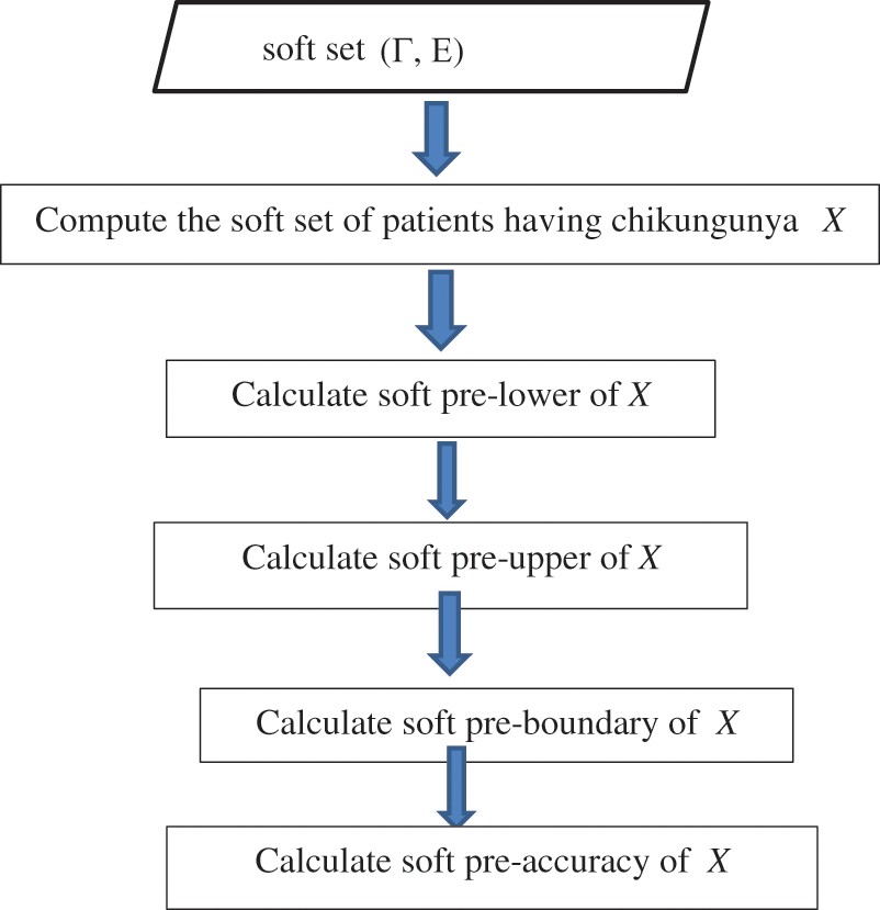
Figure 1: Framework of the proposed method
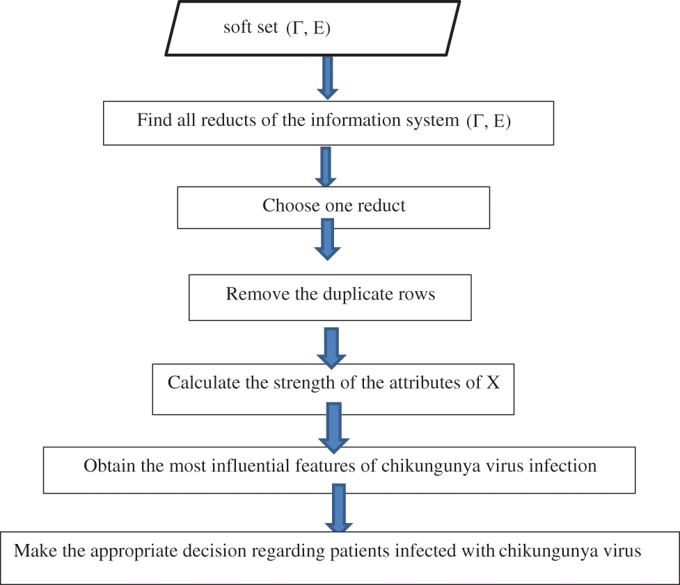
Figure 2: Framework of the result of the proposed method
4 Chikungunya Medical Application
Here we explore the problem of chikungunya, a disease that has been spread by Aedes mosquitoes that carry a virus that infects humans. CHIKV epidemics have occurred recently, linked to serious diseases. It generates a high temperature as well as significant joint discomfort. Muscle discomfort, headaches, and nausea are some of the other symptoms. The first signs and symptoms are similar to those of dengue fever. It typically does not endanger one's life. However, joint discomfort might linger for a long time. It might take months for you to fully heal. In most cases, the patient develops lifetime immunity to infection, making re-infection extremely unlikely. The illness has expanded throughout Africa and Asia in recent decades, particularly the subcontinent of India. Observe the table below, which contains information on 8-patients.
The following is a description of a set-valued information system in Table 1:
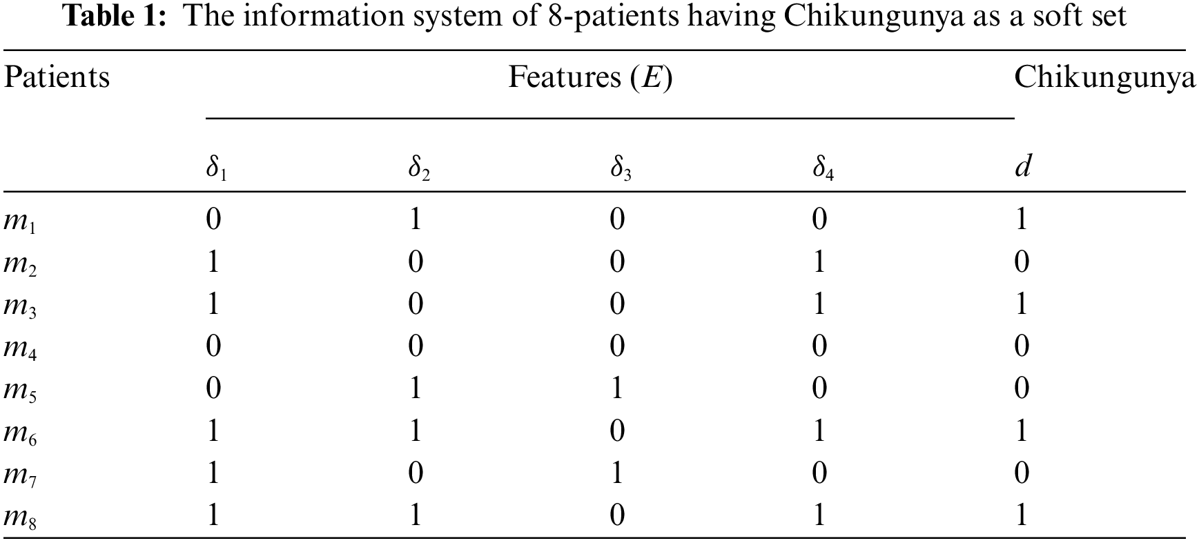
Let
In this section, the rules will be generated depending on the reduct. and core as in Table 1, since the reduct sets are
Similarly, the strength of rule
Similarly, the strength of rule
Finally, we can find the strength of rules
Then, from the above calculations we find that the attributes
Core attributes one removal with MATLAB program [22]. Next, we get Remove Themes as the next Table 2.
From this Table 2, we find the core of this table in such a method remains consistent if we delete the value
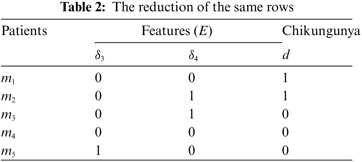
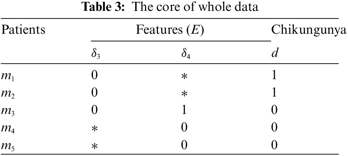
Thus, Table 3 shows that the core of the whole Table 1 This enables us to reduce to Table 3 by merging duplicate rows. We can eliminate the identical rows and get the following Table 4.
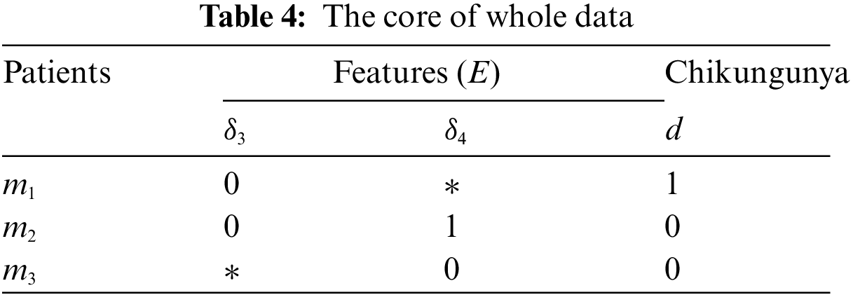
Table 4 gives us the decision rules based on the reduction as follows: if
In this article, we introduce the characteristics of the approach soft pre-rough set approximation and its decision making. We have introduced a new definition of this approach namely, soft pre-rough equality, soft pre-rough inclusion, soft pre-lower, soft pre-upper belong, soft pre-dense, soft pre-nowhere dense, soft pre-residual, soft pre-external lower and soft pre-internal upper and we also study some of their properties. We used our novel approach to identify the most important trait on the basis of its strength, which is an important method for analytical approach and decision making for any real-life problems. Also, we made a medical application to illustrate our method. This application can be used on any number of patients, any life problem and comment on the decision. Finally, the applicable technique is applied to a case study of a topological concept development strategy from the perspective of chikungunya virus in nature to validate the proposed method, as well as some comparison evaluations. We have explained our method with two algorithms and how to apply it using MATLAB. In reality, our suggestion is helpful in solving any future real-life problems. In the future, we shall extend the proposed methods to a variety of other concepts, such as the fuzzy set and fuzzy rough set.
Acknowledgement: The authors are thankful to the Deanship of Scientific Research at Najran University for funding this work under the General Research Funding Program Grant Code (NU/-/SERC/10/603).
Funding Statement: This research work is supported by the Deanship of the Scientific Research at Najran University, Najran, Saudi Arabia [NU/-/SERC/10/603].
Conflicts of Interest: The authors declare that they have no conflicts of interest to report regarding the present study.
1. El Safty, M. A. (2021). Modeling uncertainty knowledge of the topological methods. Poincare Journal of Analysis & Applications, 8(1), 1–14. DOI 10.33786/pjaa.2021.v08i01(i). 009. [Google Scholar] [CrossRef]
2. El Safty, M. A., El Sayed, M., Alblowi, S. A. (2021). Accuracy based on simply* alpha open set in rough set and topological space. Soft Computing, 25(16), 10609–10615. DOI 10.1007/s00500-021-05935-7. [Google Scholar] [CrossRef]
3. Ali, A., Ali, M. I., Rehman, N. (2019). Soft dominance based rough sets with applications in information systems. International Journal of Approximate Reasoning, 113, 171–195. DOI 10.1016/j.ijar.2019.06.009. [Google Scholar] [CrossRef]
4. Molodtsov, D. A. (1999). Soft set theory-first results. Computers & Mathematics with Applications, 37(4–5), 19–31. DOI 10.1016/S0898-1221(99)00056-5. [Google Scholar] [CrossRef]
5. Babitha, K. V., Sunil, J. J. (2016). Soft topologies generated by soft set relations. In: Handbook of researchon generalized and hybrid set structures and applications for soft computing, pp. 118–126. Calicut, India: Academic Press. DOI 10.4018/978-1-4666-9798-0.ch007. [Google Scholar] [CrossRef]
6. El-Sayed, M., El-Bably, M. K. (2017). Soft simply open set in soft topological space. Journal of Computational and Theoretical Nanoscience, 14(8), 4104–4113. DOI 10.1166/jctn.2017.6792. [Google Scholar] [CrossRef]
7. El Sayed, M. A., Alblowi, S. A., Almalki, Y., El Sayed, M. (2022). Coronavirus decision-making based on a locally simply*alpha generalized closed set. Intelligent Automation & Soft Computing, 32(1), 483–498. DOI 10.32604/iasc.2022.021581. [Google Scholar] [CrossRef]
8. El Sayed, M., Al Qubati, A. Q., El-Bably, M. K. (2020). Soft pre-rough sets and its applications in decision making. Mathematical Biosciences and Engineering, 17(5), 6045–6063. DOI 10.3934/mbe.2020321. [Google Scholar] [CrossRef]
9. Shabir, M., Ali, M. I., Shaheen, T. (2013). Another approach to soft rough sets. Knowledge-Basis Systems, 40, 72–80. DOI 10.1016/j.knosys.2012.11.012. [Google Scholar] [CrossRef]
10. El Safty, M. A., AL Zahrani, S., El-Bably, M. K., El Sayed, M. (2022). Soft xi-rough set and its applications in decision making of coronavirus. Computers, Materials & Continua, 70(1), 267–285. DOI 10.32604/cmc.2022.019345. [Google Scholar] [CrossRef]
11. Sai, B. V. S. T. (2020). Applications of soft set-in decision-making problems. Global Journal of Pure and Applied Mathematics, 16(2), 305–324. DOI 10.37622/GJPAM/16.2.2020.305-324. [Google Scholar] [CrossRef]
12. Ping, J., Atef, N., Khalil, A. M., Riaz, M., Hassan, N. (2021). Soft rough q-rung orthopair m-polar fuzzy sets and q-rung orthopair m-polar fuzzy soft rough sets and their applications. IEEE Access, 9, 139186–139200. DOI 10.1109/ACCESS.2021.3118055. [Google Scholar] [CrossRef]
13. Sahu, R., Dash, S. R., Das, S. (2021). Career selection of students using hybridized distance measure based on picture fuzzy set and rough set theory. Decision Making: Applications in Management and Engineering, 4(1), 104–126. DOI 10.31181/dmame180101P. [Google Scholar] [CrossRef]
14. Liu, Y., Qin, K., Martínez, L. (2018). Improving decision making approaches based on fuzzy soft sets and rough soft sets. Applied Soft Computing, 65, 320–332. DOI 10.1016/j.asoc.2018.01.012. [Google Scholar] [CrossRef]
15. Maji, P. K., Biswas, R., Roy, A. R. (2003). Soft set theory. Computers and Mathematics with Applications, 45(4–5), 555–566. DOI 10.1016/S0898-1221(03)00016-6. [Google Scholar] [CrossRef]
16. Maji, P. K., Roy, A. R., Biswas, R. (2002). An application of soft sets in a decision-making problem. Computer Mathematical Applications, 44, 1077–1083. DOI 10.1016/S0898-1221(02)00216-X. [Google Scholar] [CrossRef]
17. Feng, F., Liu, X., Fotea, V. L., Jun, Y. B. (2011). Soft sets and soft rough sets. Information Sciences, 181(6), 1125–1137. DOI 10.1016/j.ins.2010.11.004. [Google Scholar] [CrossRef]
18. Pawlak, Z. (1982). Rough sets. International Journal of Information Computer Science, 11(5), 341–356. DOI 10.1007/BF01001956. [Google Scholar] [CrossRef]
19. Ali, M. I. (2011). A note on soft sets, rough soft sets and fuzzy soft sets. Applied Soft Computing, 11, 3329–3332. DOI 10.1016/j.asoc.2011.01.003. [Google Scholar] [CrossRef]
20. Sharma, H. K., Kumari, K., Kar, S. (2020). A rough set approach for forecasting models. Decision Making Applications in Management and Engineering, 3(1), 1–21. DOI 10.31181/dmame2003001s. [Google Scholar] [CrossRef]
21. Sun, Q. M., Zhang, Z. L., Liu, J. (2008). Soft sets and soft modules. Rough Sets and Knowledge Technology, 5009, 403–409. DOI 10.1007/978-3-540-79721-0_56. [Google Scholar] [CrossRef]
22. El Safty, M. A., Mousa, A. A., Alblowi, S. A., El Sayed, M. (2020). Topological approach on fuzzy soft
23. Tanay, B., Kandemir, M. B. (2011). Topological structure of fuzzy soft sets. Computers and Mathematics with Application, 61(10), 2952–2957. DOI 10.1016/j.camwa.2011.03.056. [Google Scholar] [CrossRef]
24. Shakiba, A., Hooshmandasl, M. R., Davvaz, B., Fazeli, S. A. (2017). S-Approximation spaces: A fuzzy approach. Iranian Journal of Fuzzy Systems, 14(2), 127–154. DOI 10.22111/ijfs.2017.3137. [Google Scholar] [CrossRef]
25. Alblowi, S. A., El Sayed, M., El Safty, M. A. (2021). Decision making based on fuzzy soft sets and its application in COVID-19. Intelligent Automation & Soft Computing, 30(3), 961–972. DOI 10.32604/iasc.2021.018242. [Google Scholar] [CrossRef]
26. El Safty, M. A., AL Zahrani, S., Ahmar, A. S., El Sayed, M. (2022). Decision making on fuzzy soft simply* continuous of fuzzy soft multi-function. Computer Systems Science and Engineering, 40(3), 881–894. DOI 10.32604/csse.2022.019549. [Google Scholar] [CrossRef]
 | This work is licensed under a Creative Commons Attribution 4.0 International License, which permits unrestricted use, distribution, and reproduction in any medium, provided the original work is properly cited. |