| Computer Modeling in Engineering & Sciences |
DOI: 10.32604/cmes.2022.020755
ARTICLE
The Improved Element-Free Galerkin Method for Anisotropic Steady-State Heat Conduction Problems
1School of Applied Science, Taiyuan University of Science and Technology, Taiyuan, 030024, China
2Department of Civil Engineering, School of Mechanics and Engineering Science, Shanghai University, Shanghai, 200444, China
*Corresponding Author: Miaojuan Peng. Email: mjpeng@shu.edu.cn
Received: 10 December 2021; Accepted: 24 January 2022
Abstract: In this paper, we considered the improved element-free Galerkin (IEFG) method for solving 2D anisotropic steady-state heat conduction problems. The improved moving least-squares (IMLS) approximation is used to establish the trial function, and the penalty method is applied to enforce the boundary conditions, thus the final discretized equations of the IEFG method for anisotropic steady-state heat conduction problems can be obtained by combining with the corresponding Galerkin weak form. The influences of node distribution, weight functions, scale parameters and penalty factors on the computational accuracy of the IEFG method are analyzed respectively, and these numerical solutions show that less computational resources are spent when using the IEFG method.
Keywords: Improved element-free Galerkin method; penalty method; weak form; anisotropic steady-state heat conduction; improved moving least-squares approximation
Heat conduction in anisotropic material has been widely applied in various branches of science and engineering. Unlike those of isotropic materials, the thermal conductivity of anisotropic materials varies with direction. Due to the complexity of such problems, analytical solutions are limited to only a few idealized cases. Therefore, how to obtain the internal temperature distribution of anisotropic materials effectively and accurately is one of the significant directions in scientific research.
Currently, lots of meshless methods have been applied for researching heat conduction in anisotropic materials, such as local meshless method [1], regularized meshless method [2], radial basis integral equation method [3], meshless singular boundary method [4], radial basis function method [5], and so on. Compared with the traditional finite element method, a meshless method [6–9] needs only the distribution of discrete nodes, which can avoid the meshing-related drawbacks. Thus, the great precision of numerical solutions can be obtained.
As an important meshless method, the EFG method [10] was studied in 1994, in this method, the shape function was constructed by using the MLS approximation [11]. However, the disadvantage of the singular matrix often occurs in this method.
In order to eliminate the singular matrices, Cheng et al. studied the IMLS approximation [12] in 2003, thus the IEFG method was applied for many problems, such as advection-diffusion [13], elastoplasticity [14], diffusional drug release [15] problems, and so on. Under the similar computational accuracy, the IEFG method has the advantage of higher calculation speed.
By introducing the singular weight function into the MLS approximation, Lancaster et al. studied the interpolating MLS method [11], thus the boundary condition can be enforced directly in corresponding meshless method. Ren et al. improved the interpolating MLS method [16], thus the corresponding interpolating EFG method was presented [17]. Additionally, some mechanics problems [18–20] were analyzed by using this method. Qin et al. developed the interpolating smoothed particle method [21].
Using the nonsingular weight function, Wang et al. developed the improved interpolating MLS method, using this method to construct the trial function, thus the improved interpolating EFG method are presented [22], and some large deformation problems [23–25] were analyzed by using this method.
By combining the traditional finite difference method with various kinds of meshless methods, thus the hybrid EFG method [26–29], the dimensional splitting complex variable EFG method [30–34], the dimension split reproducing kernel particle method [35–38] and the hybrid generalized interpolated EFG method [39] are proposed respectively, these methods can solve the multi-dimensional problems efficiently.
In this study, the IEFG method is used for solving anisotropic steady-state heat conduction problem. The shape functions are established by using the IMLS approximation, using the penalty method to enforce the boundary condition, thus the final formulae of discretized equations of the IEFG method for anisotropic steady-state heat conduction problem can be derived by combining with the corresponding Galerkin weak form.
The influences of nodes number, weight functions, scale parameters and penalty factors on computational accuracy of the IEFG method are discussed by given examples, and numerical solutions show that the IEFG method for anisotropic steady-state heat conduction problems is convergent, compared with the traditional EFG method, less computational resources are spent when using the IEFG method.
For an arbitrary function
where
is coefficient vector of
In general,
The local approximation is
Define
where
Eq. (6) can be written as
where
and
From
we have
where
Eq. (12) sometimes forms singular or ill-conditional matrix. In order to make up for this deficiency, for basis functions
using Gram-Schmidt process, we can obtain
and
Then from Eq. (12),
where
Substituting Eq. (18) into Eq. (5), we have
where
is the shape function.
This is the IMLS approximation [12].
3 The IEFG Method for 2D Anisotropic Steady-State Heat Conduction Problems
The governing equation is
the boundary conditions are
where
The equivalent functional of anisotropic steady-state heat conduction problems is
By applying the penalty method to enforce the boundary conditions, we can obtain
where
Let
the following weak form can be obtained
where
In the problem domain, we select M nodes
From the IMLS approximation, we can obtain
where
From Eqs. (29), (30) and (32), we have
where
Substituting Eqs. (32), (34) and (35) into Eq. (28) yields
Analyzing all terms in Eq. (40), respectively, we can obtain
Let
Substituting Eqs. (41)–(45) into Eq. (40), we have
the
where
This is the IEFG method for 2D anisotropic steady-state heat conduction problem.
The formula of the relative error is
where
For simplicity, we select linear basis function in this section, and 4 × 4 Gaussian points are selected in each integral grid. Fourth numerical examples are presented, and the IEFG and the EFG methods are used to solve them, respectively.
The first example is
the boundary conditions are
The problem domain is Ω = [0, 1] × [0, 1], and
is the exact solution.
In order to illustrate the advantages of the IEFG method for 2D anisotropic steady-state heat conduction problem, we should study the convergence of this method.
Using the IEFG method to solve it, the cubic spline weight function is selected, dmax = 1.19, α = 6.0 × 10⁵, Fig. 1 shows the relationship between relative errors of numerical solutions and nodes number. It is shown that, with the increase of nodes, the precision of numerical solutions will improve as well. Thus, the numerical solution of the IEFG method in this paper is convergent.
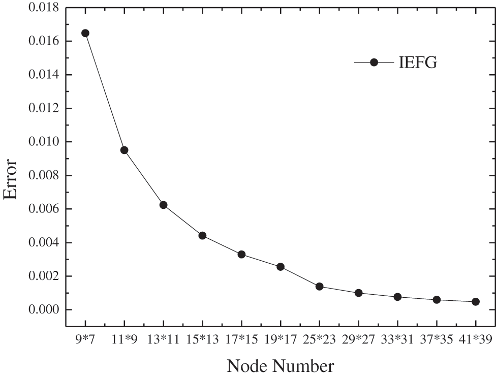
Figure 1: The error of numerical solutions of the IEFG method with the increase of nodes
The influences of weight function, scale parameter and penalty factor on solution of the IEFG method will be discussed, respectively.
1) Weighting function
If we select the cubic spline function, 17 × 15 regular nodes and 16 × 14 integral grids are selected respectively, α = 6.0 × 10⁵, dmax = 1.19, thus the smaller relative error is 0.3292%. When the quartic spline function is used, same nodes and integral grids are used respectively, α = 4.0 × 10⁵, dmax = 1.15, thus the smaller relative error is 0.3320%. It is shown that the relative error is slightly bigger when using the quartic spline function. In this section, we select the cubic spline function.
2) Scale parameter dmax
The same nodes and integral grids are used respectively, α = 4.0 × 10⁵, and the cubic spline function is used. Fig. 2 shows the relationship between dmax and relative error. It is shown that, when dmax = 1.19, the smaller relative error is obtained.
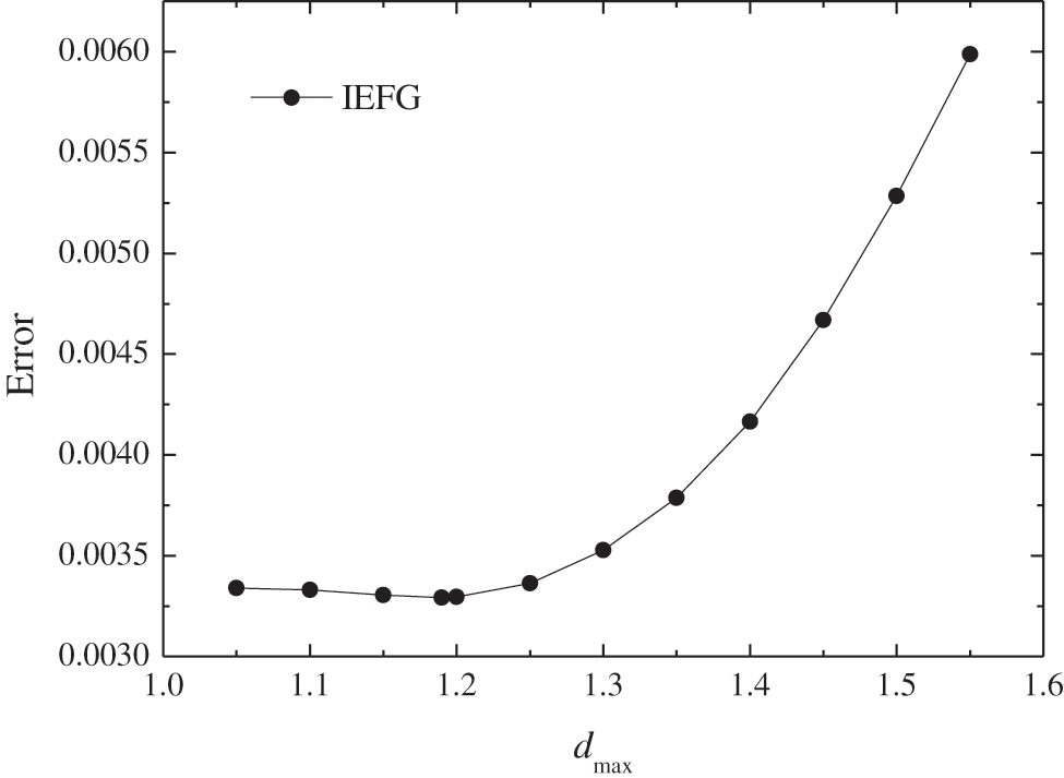
Figure 2: The error of numerical solutions of the IEFG method with the increase of dmax
3) Penalty factor α
The same nodes, integral grids and the weight function are used respectively, dmax = 1.19, Fig. 3 shows the relationship between α and relative error. It is shown that, when α=1.0 × 10⁵∼1.0 × 10⁶, the smaller relative error is obtained.
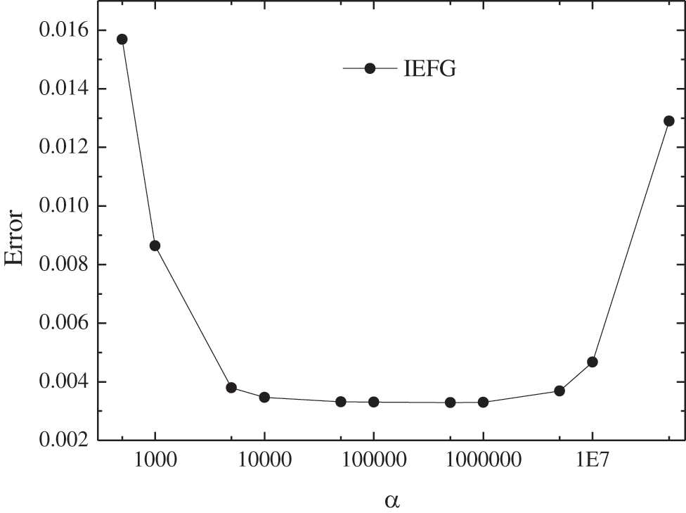
Figure 3: The error of numerical solutions of the IEFG method for different α
When the IEFG method is used to solve it, 17 × 15 regular nodes and 16 × 14 integral grids are selected, dmax = 1.19, α = 6.0 × 10⁵, and the cubic spline weight function is used; when the EFG method is used, keep all parameters consistent with the IEFG method, thus the same computational accuracy can be obtained, and the relative errors of two methods are equal to 0.3292%.
Figs. 4–7 show the comparison of numerical results and analytical ones. It is shown that the numerical solutions of two methods are in agreement very well with analytical one. The CPU times of the EFG and the IEFG methods are 0.61 and 0.51 s, respectively. Compared with the EFG method, the calculation speed of the IEFG method is slightly faster.
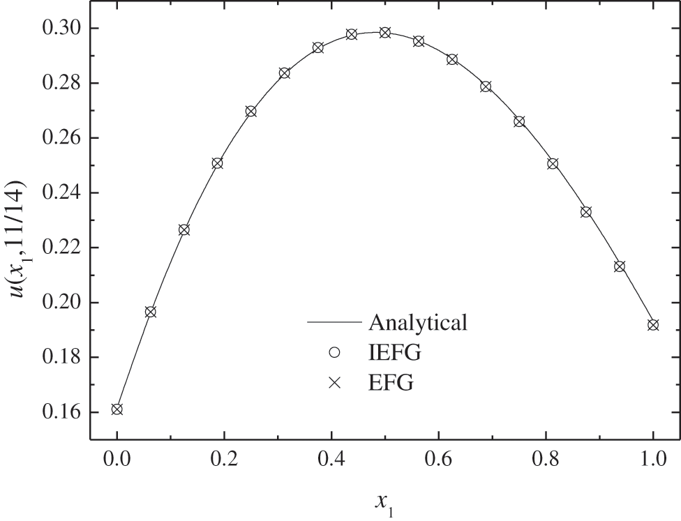
Figure 4: The comparison of numerical solutions and analytical ones along x1-axis
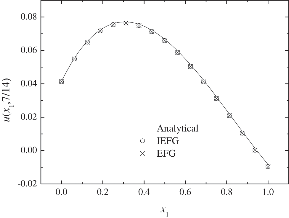
Figure 5: The comparison of numerical solutions and analytical ones along x1-axis
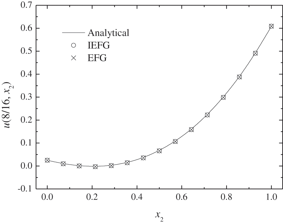
Figure 6: The comparison of numerical solutions and analytical ones along x2-axis
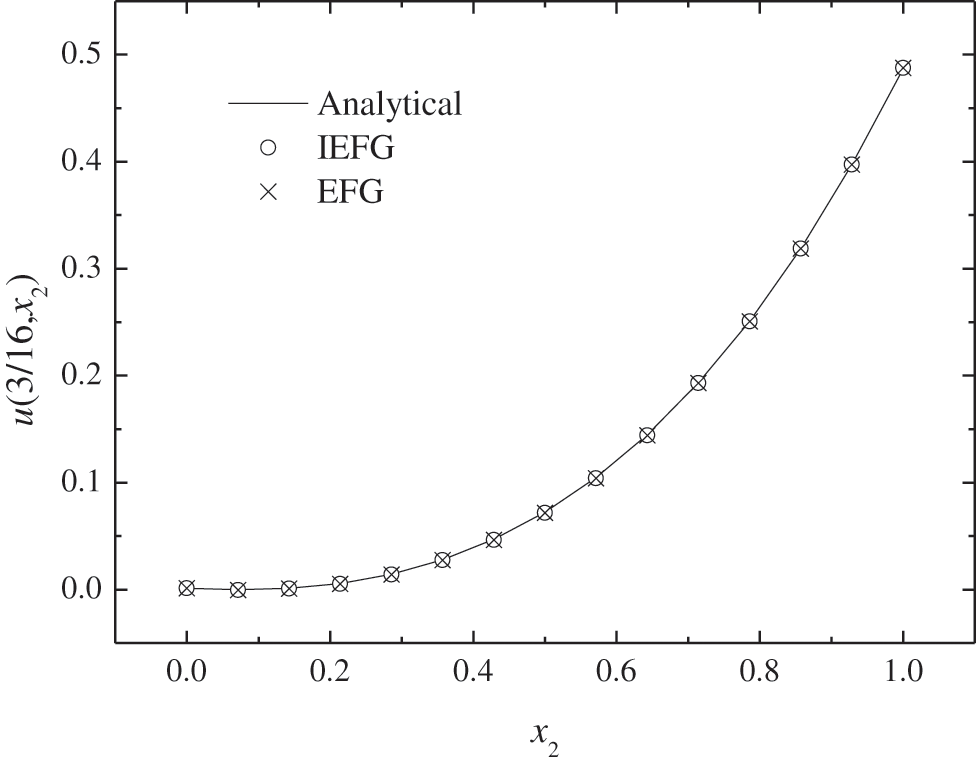
Figure 7: The comparison of numerical solutions and analytical ones along x2-axis
The second example we considered is an orthotropic medium, and the problem domain is a semi-circular ring, the outer and inner radii are 2 and 1, respectively. The governing equation is
the boundary conditions are
The problem domain is
is the exact solution.
Using the IEFG method to solve it, 21 × 11 nodes (see Fig. 8) and 20 × 10 integral grids are selected respectively, dmax = 1.7, α = 1.0 × 10³, and the cubic weight function is used, thus the smaller relative error is 0.0735%; when the EFG method is used to solve it, keep all parameters consistent with the IEFG method, thus the same calculation accuracy is obtained. The CPU times of the EFG and the IEFG methods are 1.5 and 1.1 s, respectively.
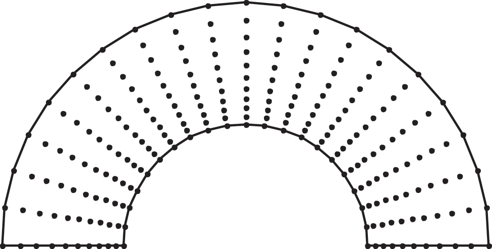
Figure 8: Nodes distributed on the problem domain
Figs. 9–12 show that the numerical results are in agreement very well with analytical one. Obviously, the advantage of the IEFG method is its faster calculation speed.
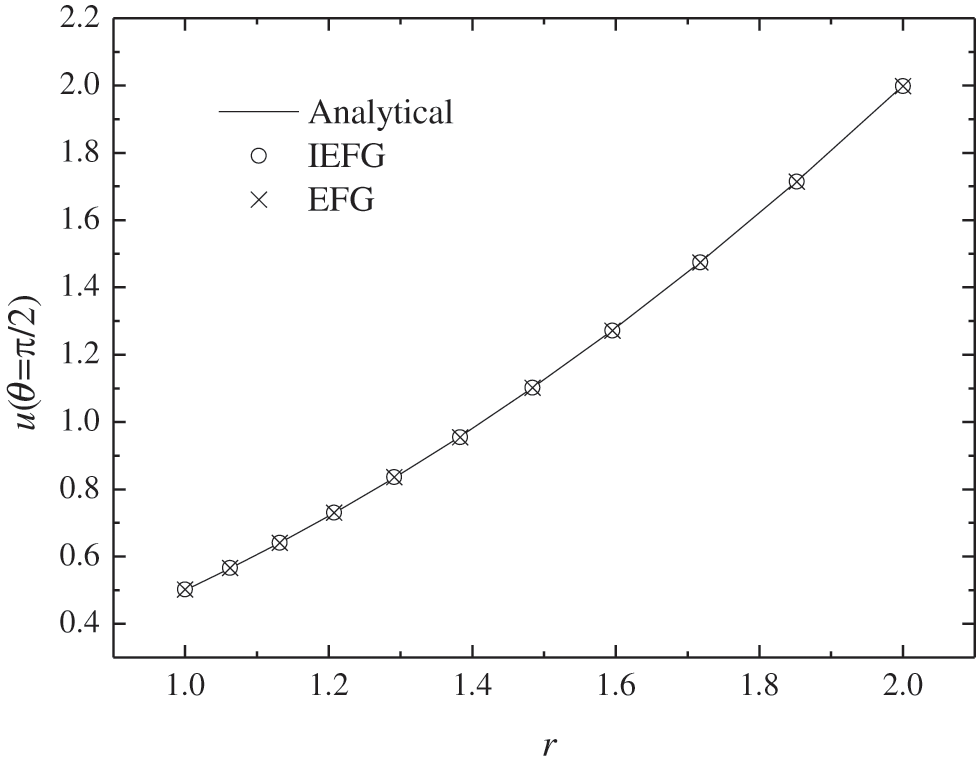
Figure 9: The comparison of numerical solutions and analytical ones when θ = π/2
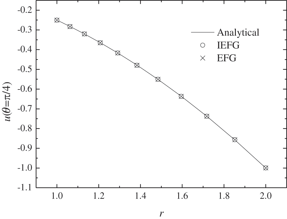
Figure 10: The comparison of numerical solutions and analytical ones when θ = π/4
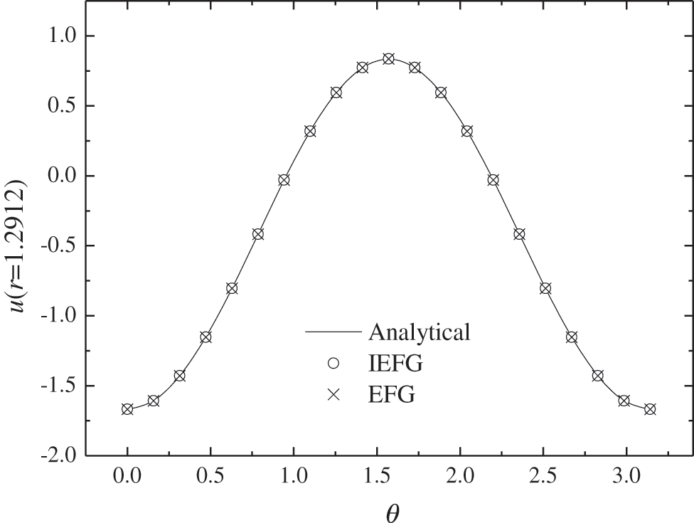
Figure 11: The comparison of numerical solutions and analytical ones at the fifth node with the direction of r
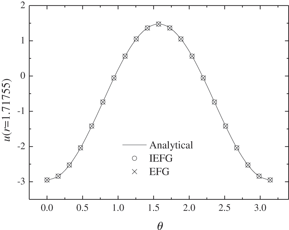
Figure 12: The comparison of numerical solutions and analytical ones at the ninth node with the direction of r
The third example is a heat conduction problem in orthotropic material with internal heat source
the boundary conditions are
The problem domain is Ω = [0, 1] × [0, 1], and
is the exact solution.
Using the IEFG method to solve it, 11 × 11 regular nodes and 10 × 10 integral grids are selected respectively, dmax = 1.2, α = 8.0 × 10³, the cubic spline weight function is used; when the EFG method is used, keep all parameters consistent with the IEFG method, thus the relative errors of both methods are equal to 0.0019%.
Figs. 13–14 show the comparison of numerical solutions and analytical ones. It is shown that the numerical results are in agreement very well with analytical one. The CPU times of the EFG and the IEFG methods are 0.4 and 0.3 s, respectively. Obviously, the IEFG method has slightly faster calculation speed than the EFG method.
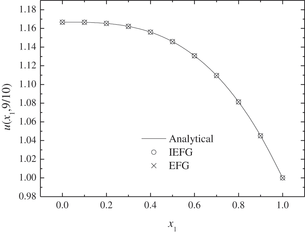
Figure 13: The comparison of numerical solutions and analytical ones along x1-axis
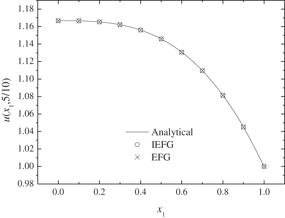
Figure 14: The comparison of numerical solutions and analytical ones along x1-axis
The fourth example is
the boundary conditions are
The problem domain is Ω=[0, 1]×[0, 1], and
is the exact solution.
When the IEFG method is used to solve it, 15 × 15 regular nodes and 14 × 14 integral grids are selected, respectively, the cubic spline weight function is used, dmax = 1.3, α = 6.0 × 10³, thus the relative error is 0.0517%; when the EFG method is used, keep all parameters consistent with the IEFG method, thus the same calculation accuracy is obtained.
Figs. 15–18 show the comparison of numerical solutions and analytical ones, it is shown that the numerical results are in agreement very well with analytical one. The CPU times of the EFG and the IEFG methods are 0.53 and 0.47 s, respectively. Thus, the IEFG method can solve it with less computational resources.
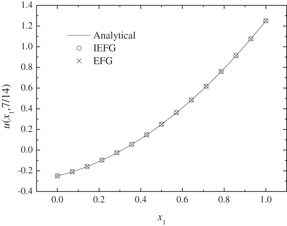
Figure 15: The comparison of numerical solutions and analytical ones along x1-axis
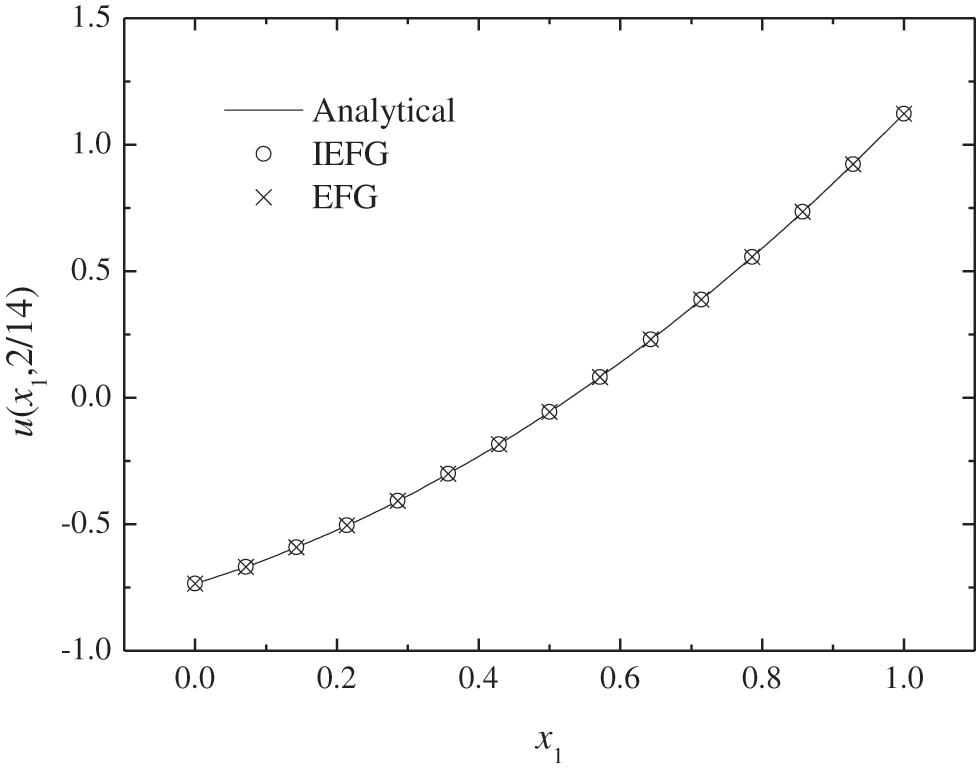
Figure 16: The comparison of numerical solutions and analytical ones along x1-axis
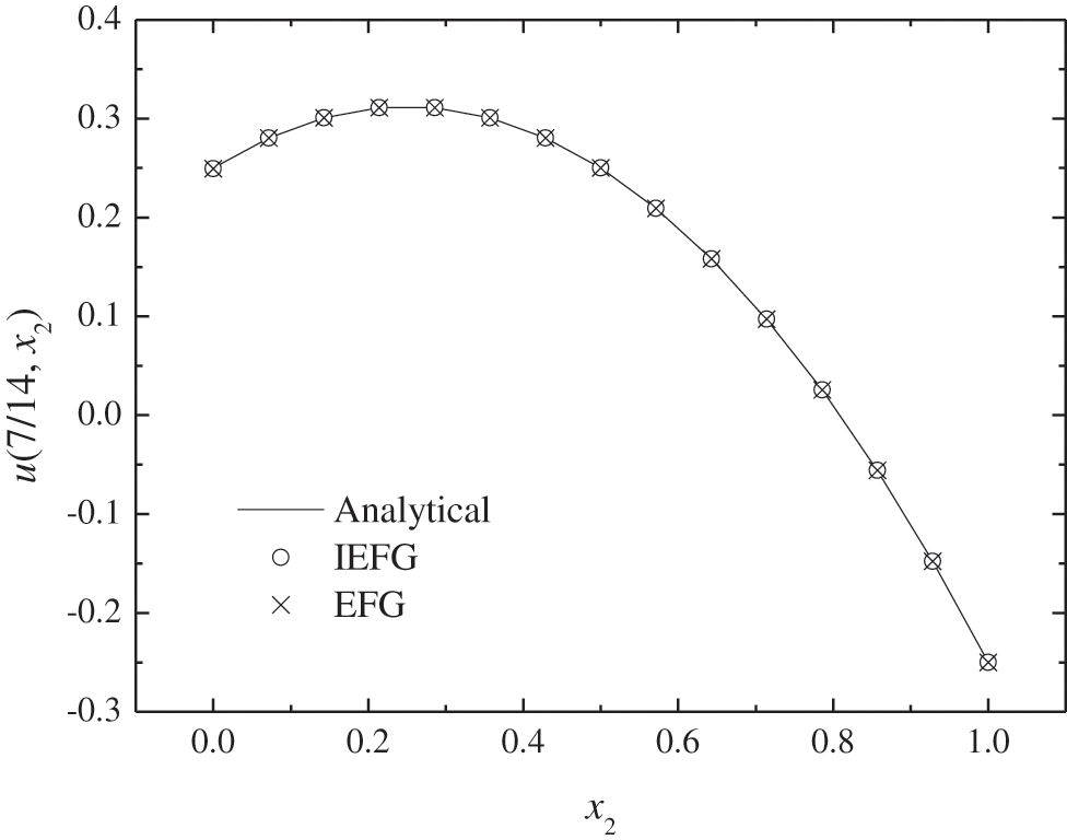
Figure 17: The comparison of numerical solutions and analytical ones along x2-axis
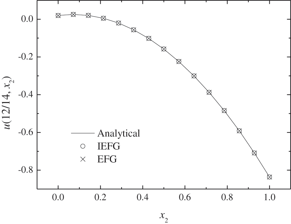
Figure 18: The comparison of numerical solutions and analytical ones along x2-axis
In order to compare the accuracy and efficiency of the IEFG and the EFG methods under different node distributions, we only change the parameters of the EFG method. When the EFG method is used, 8 × 8 regular nodes and 7 × 7 integral grids are selected, respectively, dmax = 1.27, α = 1.4 × 10³, thus the smaller relative error is 0.2274%, and the CPU time is 0.23 s. Figs. 19–20 show the comparison of numerical solutions and analytical ones. It is shown that the IEFG method has higher numerical accuracy under the condition of more nodes distribution with more computational resources.
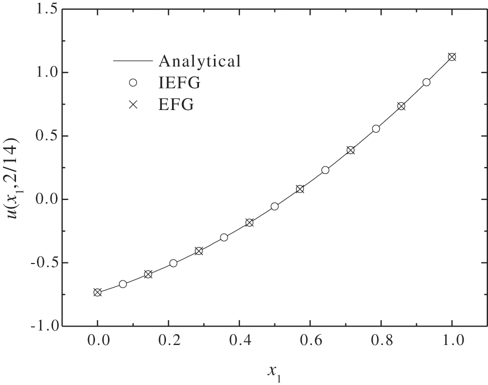
Figure 19: The comparison of numerical solutions and analytical ones along x1-axis
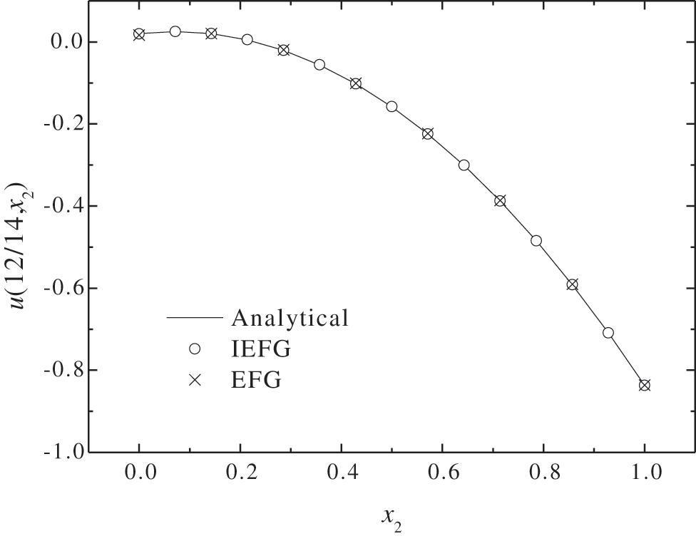
Figure 20: The comparison of numerical solutions and analytical ones along x2-axis
In this paper, we considered the IEFG method for solving 2D anisotropic steady-state heat conduction problems.
From Section 4, the good convergence of the solutions of the IEFG method is verified numerically. Moreover, the IEFG method can solve anisotropic steady-state heat conduction problems with less computational resources, and can be considered as a competitive alternative for solving science and engineering problems.
Therefore, the study in this paper can broaden the scope of application of the IEFG method.
Funding Statement: This work was supported by Natural Science Foundation of Shanxi Province (Grant No. 20210302124388).
Conflicts of Interest: The authors declare that they have no conflicts of interest to report regarding the present study.
1. Ahmadi, I., Sheikhy, N., Aghdam, M. M., Nourazar, S. S. (2010). A new local meshless method for stead-state heat conduction in heterogeneous materials. Engineering Analysis with Boundary Elements, 34(12), 1105–1112. DOI 10.1016/j.enganabound.2010.06.012. [Google Scholar] [CrossRef]
2. Sun, L. L., Chen, W., Zhang, C. Z. (2013). A new formulation of regularized meshless method applied to interior and exterior anisotropic potential problems. International Journal of Heat and Mass Transfer, 37(12–13), 7452–7464. DOI 10.1016/j.apm.2013.02.036. [Google Scholar] [CrossRef]
3. Ooi, E. H., Ooi, E. T., Ang, W. T. (2015). Numerical investigation of the meshless radial basis integral equation method for solving 2D anisotropic potential problems. Engineering Analysis with Boundary Elements, 53, 27–39. DOI 10.1016/j.enganabound.2014.12.004. [Google Scholar] [CrossRef]
4. Gu, Y., Chen, W., Zhang, C. Z., He, X. Q. (2015). A meshless singular boundary method for three-dimensional inverse heat conduction problems in general anisotropic media. International Journal of Heat and Mass Transfer, 84, 91–102. DOI 10.1016/j.ijheatmasstransfer.2015.01.003. [Google Scholar] [CrossRef]
5. Reutskiy, S. Y. (2016). A meshless radial basis function method for 2D steady-state heat conduction problems in anisotropic and inhomogeneous media. Engineering Analysis with Boundary Elements, 66, 1–11. DOI 10.1016/j.enganabound.2016.01.013. [Google Scholar] [CrossRef]
6. Li, S., Liu, W. K. (2004). Meshfree particle methods. Germany: Springer-Verlag. [Google Scholar]
7. Liu, W. K., Jun, S., Li, S. F., Adee, J., Belytschko, T. (1995). Reproducing kernel particle methods for structural dynamics. International Journal of Numerical Methods for Engineering, 38, 1655–1679. DOI 10.1002/nme.1620381005. [Google Scholar] [CrossRef]
8. Liu, W. K., Li, S. F., Belytschko, T. (1997). Moving least-square reproducing kernel method. (I) Methodology and convergence. Computer Methods in Applied Mechanics and Engineering, 143, 113–154. DOI 10.1016/S0045-7825(96)01132-2. [Google Scholar] [CrossRef]
9. Li, S. F., Liu, W. K. (1999). Reproducing kernel hierarchical partition of unity, Part I-Formulations and theory. International Journal for Numerical Methods in Engineering, 45(3), 251–288. [Google Scholar]
10. Belytschko, T., Lu, Y. Y., Gu, L. (1994). Element-free Galerkin methods. International Journal for Numerical Methods in Engineering, 37(2), 229–256. DOI 10.1002/nme.1620370205. [Google Scholar] [CrossRef]
11. Lancaster, P., Salkauskas, K. (1981). Surface generated by moving least squares methods. Mathematics of Computation, 37(155), 141–158. DOI 10.1090/S0025-5718-1981-0616367-1. [Google Scholar] [CrossRef]
12. Cheng, Y. M., Chen, M. J. (2003). A boundary element-free method for linear elasticity. Acta Mechanica Sinica, 35(2), 181–186. [Google Scholar]
13. Cheng, H., Zheng, G. D. (2020). Analyzing 3D advection-diffusion problems by using the improved element-free Galerkin method. Mathematical Problems in Engineering, 2020, 4317538. DOI 10.1155/2020/4317538. [Google Scholar] [CrossRef]
14. Yu, S. Y., Peng, M. J., Cheng, H., Cheng, Y. M. (2019). The improved element-free Galerkin method for three-dimensional elastoplasticity problems. Engineering Analysis with Boundary Elements, 104, 215–224. DOI 10.1016/j.enganabound.2019.03.040. [Google Scholar] [CrossRef]
15. Zheng, G. D., Cheng, Y. M. (2020). The improved element-free Galerkin method for diffusional drug releas e problems. International Journal of Applied Mechanics, 12(8), 2050096. DOI 10.1142/S1758825120500969. [Google Scholar] [CrossRef]
16. Ren, H. P., Cheng, Y. M., Zhang, W. (2010). Researches on the improved interpolating moving least-squares method. Chinese Journal of Engineering Mathematics, 27(6), 1021–1029. [Google Scholar]
17. Ren, H. P., Cheng, Y. M. (2012). The interpolating element-free Galerkin (IEFG) method for two-dimensional potential problems. Engineering Analysis with Boundary Elements, 36(5), 873–880. DOI 10.1016/j.enganabound.2011.09.014. [Google Scholar] [CrossRef]
18. Wu, Q., Liu, F. B., Cheng, Y. M. (2020). The interpolating element-free Galerkin method for three-dimensional elastoplasticity problems. Engineering Analysis with Boundary Elements, 115, 156–167. DOI 10.1016/j.enganabound.2020.03.009. [Google Scholar] [CrossRef]
19. Wu, Q., Peng, P. P., Cheng, Y. M. (2021). The interpolating element-free Galerkin method for elastic large deformation problems. Science China Technological Sciences, 64(2), 364–374. DOI 10.1007/s11431-019-1583-y. [Google Scholar] [CrossRef]
20. Cheng, Y. M., Bai, F. N., Liu, C., Peng, M. J. (2016). Analyzing nonlinear large deformation with an improved element-free Galerkin method via the interpolating moving least-squares method. International Journal of Computational Materials Science and Engineering, 5(4), 1650023. DOI 10.1142/S2047684116500238. [Google Scholar] [CrossRef]
21. Qin, Y. X., Li, Q. Y., Du, H. X. (2017). Interpolating smoothed particle method for elastic axisymmetrical problem. International Journal of Applied Mechanics, 9(2), 1750022. DOI 10.1142/S1758825117500223. [Google Scholar] [CrossRef]
22. Wang, J. F., Sun, F. X., Cheng, Y. M. (2012). An improved interpolating element-free Galerkin method with nonsingular weight function for two-dimensional potential problems. Chinese Physics B, 21(9), 090204. DOI 10.1088/1674-1056/21/9/090204. [Google Scholar] [CrossRef]
23. Liu, F. B., Cheng, Y. M. (2018). The improved element-free Galerkin method based on the nonsingular weight functions for elastic large deformation problems. International Journal of Computational Materials Science and Engineering, 7(4), 1850023. DOI 10.1142/S2047684118500239. [Google Scholar] [CrossRef]
24. Liu, F. B., Wu, Q., Cheng, Y. M. (2019). A meshless method based on the nonsingular weight functions for elastoplastic large deformation problems. International Journal of Applied Mechanics, 11(1), 1950006. DOI 10.1142/S1758825119500066. [Google Scholar] [CrossRef]
25. Liu, F. B., Cheng, Y. M. (2018). The improved element-free Galerkin method based on the nonsingular weight functions for inhomogeneous swelling of polymer gels. International Journal of Applied Mechanics, 10(4), 1850047. DOI 10.1142/S1758825118500473. [Google Scholar] [CrossRef]
26. Meng, Z. J., Cheng, H., Ma, L. D., Cheng, Y. M. (2018). The dimension split element-free Galerkin method for three-dimensional potential problems. Acta Mechanica Sinica, 34(3), 462–474. DOI 10.1007/s10409-017-0747-7. [Google Scholar] [CrossRef]
27. Meng, Z. J., Cheng, H., Ma, L. D., Cheng, Y. M. (2019). The dimension splitting element-free Galerkin method for 3D transient heat conduction problems. Science China Physics, Mechanics & Astronomy, 62(4), 040711. DOI 10.1007/s11433-018-9299-8. [Google Scholar] [CrossRef]
28. Meng, Z. J., Cheng, H., Ma, L. D., Cheng, Y. M. (2019). The hybrid element-free Galerkin method for three-dimensional wave propagation problems. International Journal for Numerical Methods in Engineering, 117(1), 15–37. DOI 10.1002/nme.5944. [Google Scholar] [CrossRef]
29. Ma, L. D., Meng, Z. J., Chai, J. F., Cheng, Y. M. (2020). Analyzing 3D advection-diffusion problems by using the dimension splitting element-free Galerkin method. Engineering Analysis with Boundary Elements, 111, 167–177. DOI 10.1016/j.enganabound.2019.11.005. [Google Scholar] [CrossRef]
30. Cheng, H., Peng, M. J., Cheng, Y. M. (2018). The dimension splitting and improved complex variable element-free Galerkin method for 3-dimensional transient heat conduction problems. International Journal for Numerical Methods in Engineering, 114(3), 321–345. DOI 10.1002/nme.5745. [Google Scholar] [CrossRef]
31. Cheng, H., Peng, M. J., Cheng, Y. M. (2017). A hybrid improved complex variable element-free Galerkin method for three-dimensional potential problems. Engineering Analysis with Boundary Elements, 84, 52–62. DOI 10.1016/j.enganabound.2017.08.001. [Google Scholar] [CrossRef]
32. Cheng, H., Peng, M. J., Cheng, Y. M. (2017). A fast complex variable element-free Galerkin method for three-dimensional wave propagation problems. International Journal of Applied Mechanics, 9(6), 1750090. DOI 10.1142/S1758825117500909. [Google Scholar] [CrossRef]
33. Cheng, H., Peng, M. J., Cheng, Y. M. (2018). A hybrid improved complex variable element-free Galerkin method for three-dimensional advection-diffusion problems. Engineering Analysis with Boundary Elements, 97, 39–54. DOI 10.1016/j.enganabound.2018.09.007. [Google Scholar] [CrossRef]
34. Cheng, H., Peng, M. J., Cheng, Y. M., Meng, Z. J. (2020). The hybrid complex variable element-free Galerkin method for 3D elasticity problems. Engineering Structures, 219, 110835. DOI 10.1016/j.engstruct.2020.110835. [Google Scholar] [CrossRef]
35. Peng, P. P., Wu, Q., Cheng, Y. M. (2020). The dimension splitting reproducing kernel particle method for three-dimensional potential problems. International Journal for Numerical Methods in Engineering, 121, 146–164. DOI 10.1002/nme.6203. [Google Scholar] [CrossRef]
36. Peng, P. P., Cheng, Y. M. (2020). Analyzing three-dimensional transient heat conduction problems with the dimension splitting reproducing kernel particle method. Engineering Analysis with Boundary Elements, 121, 180–191. DOI 10.1016/j.enganabound.2020.09.011. [Google Scholar] [CrossRef]
37. Peng, P. P., Cheng, Y. M. (2021). Analyzing three-dimensional wave propagation with the hybrid reproducing kernel particle method based on the dimension splitting method. Engineering with Computers. DOI 10.1007/s00366-020-01256-9. [Google Scholar] [CrossRef]
38. Peng, P. P., Cheng, Y. M. (2021). A hybrid reproducing kernel particle method for three-dimensional advection-diffusion problems. International Journal of Applied Mechanics, 13, 2150085. DOI 10.1142/S175882512150085X. [Google Scholar] [CrossRef]
39. Wang, J. F., Sun, F. X. (2020). A hybrid generalized interpolated element-free Galerkin method for stokes problems. Engineering Analysis with Boundary Elements, 111, 88–100. DOI 10.1016/j.enganabound.2019.11.002. [Google Scholar] [CrossRef]
40. Shiah, Y. C., Tan, C. L. (1997). BEM treatment of two-dimensional anisotropic field problems by direct domain mapping. Engineering Analysis with Boundary Elements, 20, 347–351. DOI 10.1016/s0955-7997(97)00103-3. [Google Scholar] [CrossRef]
41. Luo, X., Huang, J. (2014). High-accuracy quadrature methods for solving boundary integral equations of steady-state anisotropic heat conduction problems with Dirichlet conditions. International Journal of Computer Mathematics, 91(5), 1097–1121. DOI 10.1080/00207160.2013.828050. [Google Scholar] [CrossRef]
 | This work is licensed under a Creative Commons Attribution 4.0 International License, which permits unrestricted use, distribution, and reproduction in any medium, provided the original work is properly cited. |