| Computer Modeling in Engineering & Sciences |
DOI: 10.32604/cmes.2022.020427
ARTICLE
Pollution Dispersion in Urban Street Canyons with Green Belts
1School of Energy and Power Engineering, Shandong University, Jinan, 250061, China
2CNPC Ji Chai Power Equipment Company, Jinan, 250306, China
*Corresponding Author: Li Lei. Email: leili@sdu.edu.cn
Received: 25 November 2021; Accepted: 27 December 2021
Abstract: In this study, numerical simulations were used to explore the effects of roadside green belt, urban street spatial layout, and wind speed on vehicle exhaust emission diffusion in street canyon. The diffusion of different sized particles in the street canyon and the influence of wind speed were investigated. The individual daily average pollutant intake was used to evaluate the exposure level in a street canyon microenvironment. The central and leeward green belts of the road were the most conducive to the diffusion of pollutants, while the positioning of the green belts both sides of a road was least conducive to the diffusion of pollutants. Pollutant levels increased with increasing canopy height, canopy width, and decreasing tree spacing, with optimal values of 12 m, 7 m, and 0.4 H, respectively. This provides protection from pollution for low-rise residents and pedestrians. The results presented here can be used to improve the air quality of the street microenvironment and provide a basis for the renovation of old street buildings.
Keywords: Street canyons; roadside green belts; pollutant exposure; particulate matter; fluent software
The concentration of population in cities [1,2] has resulted in rapid developments in urban architecture. Urban traffic congestion within areas of dense new and old buildings leads to large concentrations of motor vehicle pollutants in urban areas, and air quality in street canyons has become an invisible killer threatening human health and life [1–4]. In addition to CO exhaust pollution, particulate matters has often been referred to as the “winter killer”. With the frequent occurrence of haze, there is an urgent need to explore the factors controlling the diffusion and distribution of particulate matter in street canyons, and to find ways to reduce the concentration of particulate matter in the atmosphere.
Luan et al. [5] studied the influence of wind speed and direction on the diffusion of fine particles in street canyons through measurements, and determined the influence of different pollutant sources on pollutant distribution through numerical simulations [6]. Jin et al. [7] measured the particle concentration of 100 nm to 3 μm particles in a street canyon, and found that the particle concentration was related to the heat flow, traffic flow, wind speed, and wind direction, and presented a vertical gradient with increasing height below roof level. He et al. [8] used the discrete phase model (DPM) to simulate dust particles of 0.5–380 μm, and found that the particle size of 50 μm could be used as the demarcation point, with the results for particles less than 50 μm being significantly improved. A computational fluid dynamics (CFD) model based on real-world measurements was applied and used an inhalation fraction (IF) approach to simulate and explore the impact of ultrafine particulate emissions from traffic on population exposure was used in urban street canyons [9].
However, the influence of a street canyon on air quality depends on its geometry, meteorological conditions, and vegetation characteristics. It is well known that roadside greenbelt construction is an important aspect of urban design [10,11], and has many positive effects. However, recent studies have found that roadside green belts can limit the diffusion of pollutants, which will increase the concentration of pollutants in street canyons. In addition, the flow field structure and pollutant concentration in street canyons changes with the layout of roadside green belts [12–17].
Wang et al. [18] discovered that different forms of roadside green belts generated substantial differences in the PM2.5 concentration, and the presence or absence of green belts also made a significant difference to the particulate matter concentration.
Wania et al. [19] used a microclimate model, ENVI-MET, to simulate and analyze the effects of different forms of vegetation planting on particle diffusion in street canyons. The results showed that vegetation could reduce wind speed and inhibit air convection, which can increase the particulate matter concentration.
Xu et al. [20] considered roadside green belts to be a porous uniform medium and numerically simulated the diffusion and distribution of vehicle exhaust gases when there was a green belt in the center of a road using the standard K-turbulence model. The results showed that the overall wind speed in the street canyon decreased after a green belt was established, and the pollutant concentrations at the leeward side and near the canyon increased significantly. In addition, the higher the canopy base height of the green belt, the lower the wind speed and the higher the pollutant concentration in the street canyon.
A few studies have combined the effects of meteorological factors and street canyon structure on the form and arrangement of roadside green belts to determine the exposure of residents to CO at different floor heights in street canyons.
This study used an urban street canyon as the research object. It was located within the narrow streets, old cities, and buildings of the environmental protection area of the medium-sized city of Jinan, China. The study investigated how best to adjust the microclimate of street canyon, while maintaining the old city environment and enabling pedestrians and residents to experience healthy air in a congested urban area. On the basis of previous wind tunnel experiments, the influence of specific roadside green belts on vehicle exhaust emission diffusion in street canyons was comprehensively studied. At the same time, a preliminary investigation of the distribution of particulate matter in a street canyon was conducted. Carbon monoxide and particulate matter exposure for pedestrians and residents in the canyon was also measured. Reducing the pollutant concentration will improve the physical comfort of the street canyons microenvironment. The results can be used to optimize the layout of roadside green belts and effectively adjust the layout of old street canyons.
2.1 Definition of Pollutant Exposure Indexes
2.1.1 Short-Term Average Daily Exposure Dose in a Microenvironment
With consideration of the lifetime average daily exposure dose (LADD) [6,21,22], the short-term average daily exposure dose (ADD) in a microenvironment was calculated as:
where C is the exposure concentration (g/m3); IR is the respiratory rate (m3/h); ED is the short-term exposure time in the microenvironment per day (h/day); and BW is the body weight (kg).
The mean short-term average daily exposure dose (MADD) was calculated as:
where Pi is the population ratio of age groups, which is based on United Nations statistics and Chinese census data from recent years. All the ADDs referred to in the following text are MADDs unless otherwise specified.
The inhalation dose exposure parameters were determined based on characteristic human body parameters, temporal-behavior pattern parameters, respiratory rates, and other information obtained from questionnaires [1–2,23–25], with some values being different for indoor and outdoor environments. It was divided into infants aged under 6 years; children aged 7–18 years; adults aged 19–60 years and elders aged over 60 years. Their respiratory rates (m3/h) are 0.285, 0.285, 0.55, 0.58 in turn; their short-term exposure time of microenvironment (h/d) are 1.17, 0.36, 0.75, 0.35; their weights (kg) are 60.53, 14.87, 55.47, 46.45 and the population ratios (%) are 64.0, 5.8, 18.1, 12.1 accordingly. For the exposure of urban residents to Carbon monoxide and particles in the indoor environment we referred to Wu et al. [1,2].
Based on the results of the wind tunnel experiment (https://www.umweltaerodynamik.de/bilder-originale/CODA/CODASC.html), it was assumed that the canopy of the green belt was a porous medium. It was assumed that the porosity of the canopy model of the green belt was 96% (corresponding to the canopy porosity of deciduous trees).
The pore size and leaf surface properties of different tree species have different effects on the surrounding air flow. We used porosity and a pressure loss coefficient to represent the characteristics of trees. Porosity represents the density of the surface area of trees, and was determined as follows:
where V0 is the volume occupied by leaves and branches; and V is the volume covered by trees.
A pressure loss coefficient was used to describe the aerodynamic characteristics of the tree canopy, and was obtained by measuring the static pressure difference between the upstream and downstream of the porous media, the thickness of the porous media, the flow density, and the average flow velocity [26,27]. It was determined as follows:
where,
For the flow of fluid in a porous media, a momentum source term was added to the momentum equation to express the resistance to fluid movement of the porous media [28].
Momentum source term of porous media:
Yi is the source term of momentum in the i direction; and Eij and Fij represent the coefficient matrix. The momentum primary term consists of a viscous loss term and inertia loss term.
The simulation software was fluent 20RS (from Shandong University High Performance Computing Cloud Platform, Jinan, China). In the geometric model, the length-width ratio of street canyon is 10:1. Since only two-dimensional features are studied, the model is simplified to two-dimensional. Gambit software (http://www.gambit-project.org/) was used for modeling and meshing, and Tecplot was used for data post-processing. By comparing the convergence and calculation results, the standard K equation model was adopted as the turbulence model. The diffusion of pollutants was determined using the component transport equation without a chemical effect [29]. For the particulate solid phase, the DPM was used to track the diffusion of particulate matter [30], to describe the continuous phase air flow field and the trajectory of particulate matter. Particle resistance, gravity and buoyancy were considered, and other extras vary according to the environment.
2.2.3 The Validation of CFD for Pollutant Dispersion Modeling
The experimental model is shown in Fig. 1a. The length, width, and height of the experimental street canyon were 120, 12, and 12 cm, respectively. A roadside green belt was established in the center of the street canyon. The scale of the experimental model compared to a real street canyon scale was 1:150.
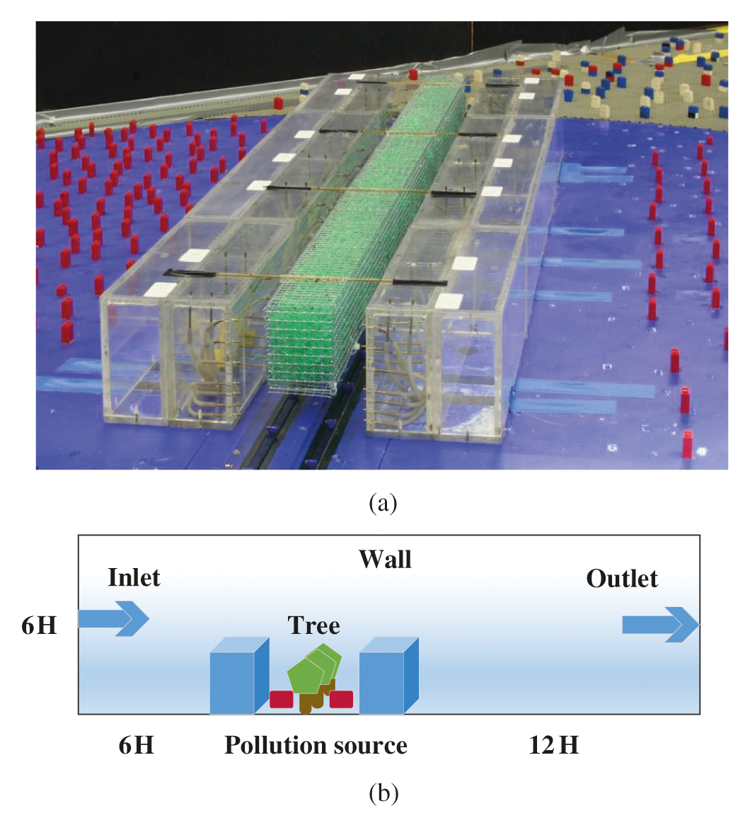
Figure 1: Schematic diagram of the numerical simulation model. (a) Wind tunnel test site (b) The two-dimensional (2D) street canyon model
In the wind tunnel test, the wind direction at the entrance was perpendicular to the axis of the street canyon, and the magnitude of the velocity followed an exponential distribution. The turbulence of the incoming flow was expressed by turbulent kinetic energy k and turbulent diffusivity ε, with the specific function expressed as follows:
where, the surface friction velocity u* = 0.52 m/s, Cμ = 0.09, the boundary layer thickness δ = 0.47 m, and K (the von Kàrmàn constant) = 0.40.
The pollutant concentration was described by K, which is a dimensionless value. It was expressed as follows:
where, Cm is the measured concentration; H represents the height of the buildings on both sides; UH represents the wind speed at z = H; Q represents the source strength; and Lq represents the length of the line source.
2.2.4 Boundary Conditions and Parameter Setting for CFD Simulations
A calculation area with a length and height of 24 × 6 H was selected as shown in Fig. 1b, in which the entrance boundary was 6 H from the upstream building, and the outflow boundary was 12 H from the downstream building. Inflow and outflow were defined as the velocity inflow and free outflow, the surfaces of the ground and buildings were set to walls. Structured grids were used in the division of the 2D model region, with the final number of grids being 250,000 after grid independence verification. A geometric schematic diagram of the street canyon used in the numerical simulation is shown in Fig. 1b.
CO was used as the pollutant. Four lanes were set in both directions in the model. Considering that the maximum allowable CO concentration in urban air according to Chinese regulations, the CO concentration from the idling engine of a single motor vehicle was set to 20 mg/m3 per hour.
The continuous phase air flow field was calculated first, and after convergence to an accuracy of 10−4, particles from a jet source were added for the coupling calculation and unsteady tracking. The density of particles was set to 2000 kg/m3 [31]. Based on the typical particulate pollution level and motor vehicle emission standards of Jinan, the source intensity was set at 2 g/s.
A 2D model was adopted to conduct simulations under four conditions: the tree crown width was kept at 9 m, and the height was set to 6, 8, 10, and 14 m in turn, as shown in Fig. 2. A comparative analysis was made with a tree crown height of 12 m as the verification scheme.
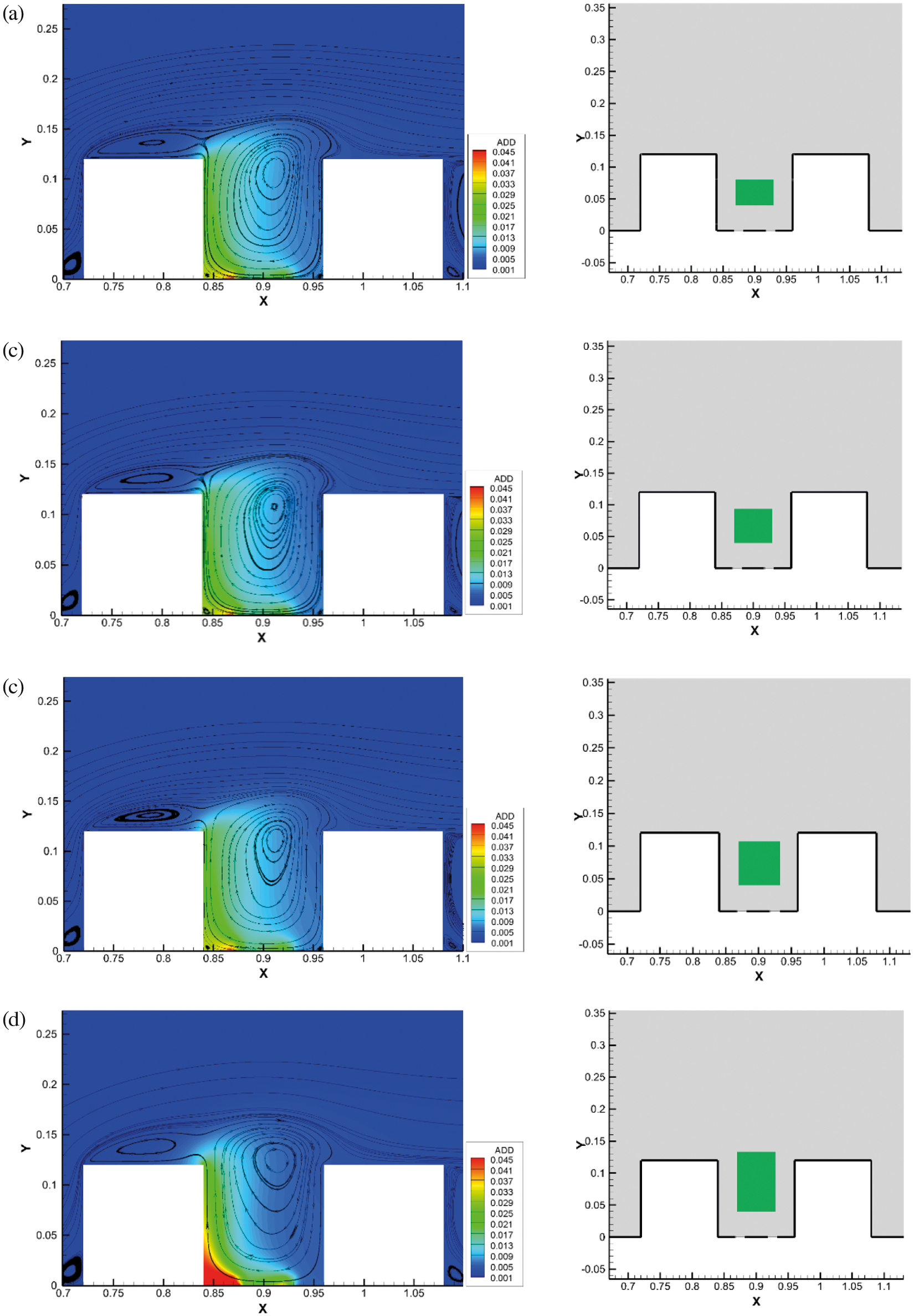
Figure 2: The short-term average daily exposure dose (ADD) contours and streamlines in schemes where the tree crown width was kept at 9 m, and the tree crown height was set to (a) 6, (b) 8, (c) 10, and (d) 14 m in turn
A 2D model was adopted, and the canopy height of the green belt was set to 12 m. The pollutant diffusion in the street canyon was simulated under four conditions, with canopy widths of 3, 5, 7, and 11 m, respectively, and was then compared with the 9 m example in the verification scheme, as shown in Fig. 3.
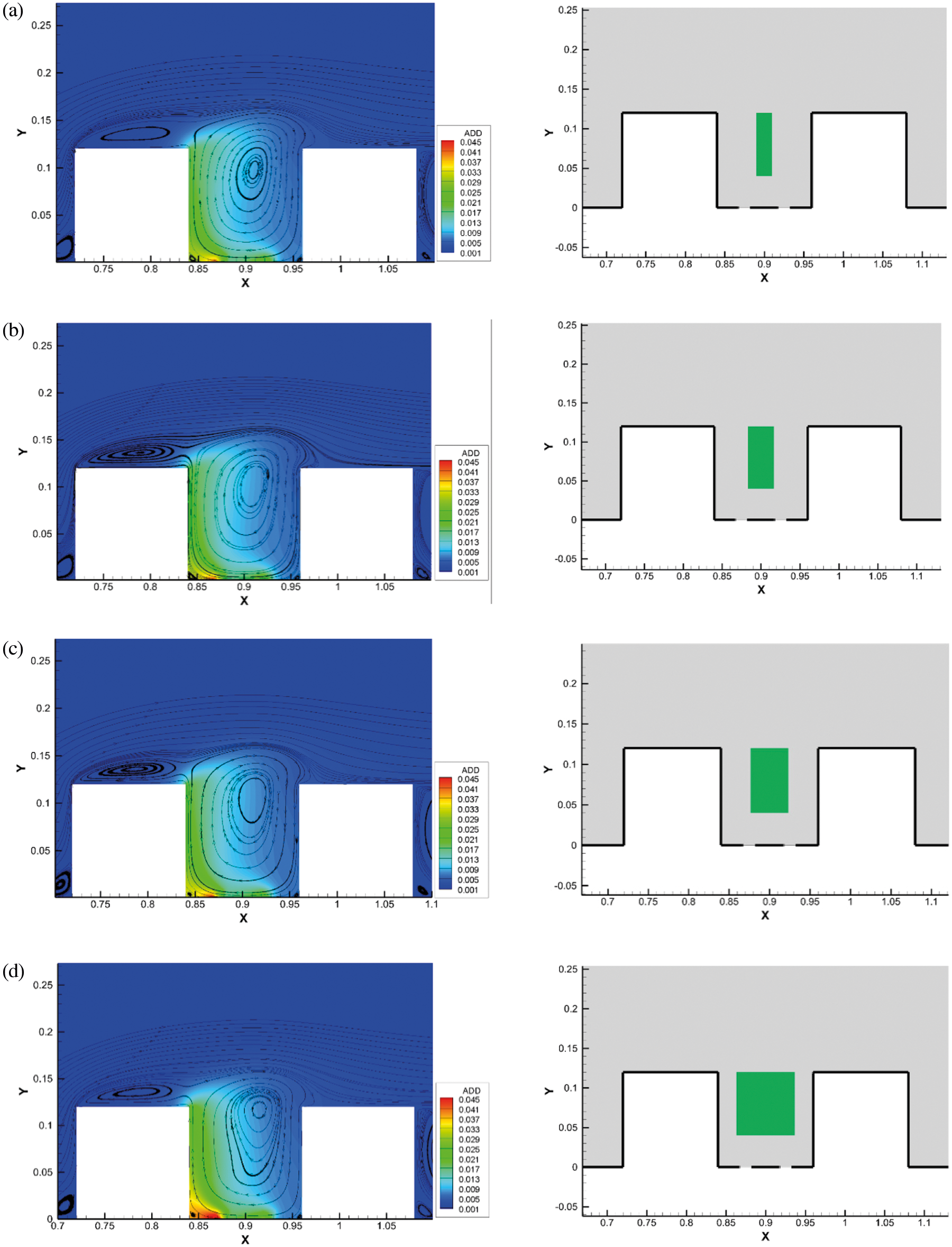
Figure 3: The short-term average daily exposure dose (ADD) contours and streamlines in the schemes where the canopy height of the green belt was set to 12 m and the canopy width was set to (a) 3, (b) 5, (c) 7, and (d) 11 m, respectively
2.3.3 Layout of Roadside Green Belt
The distribution of the air flow field and pollutant concentrations in street canyons with an aspect ratio (AR) of 1 were simulated when the green belt was established in the center of the road and on the leeward, windward, and both sides of the road in turn, as shown in Fig. 4.
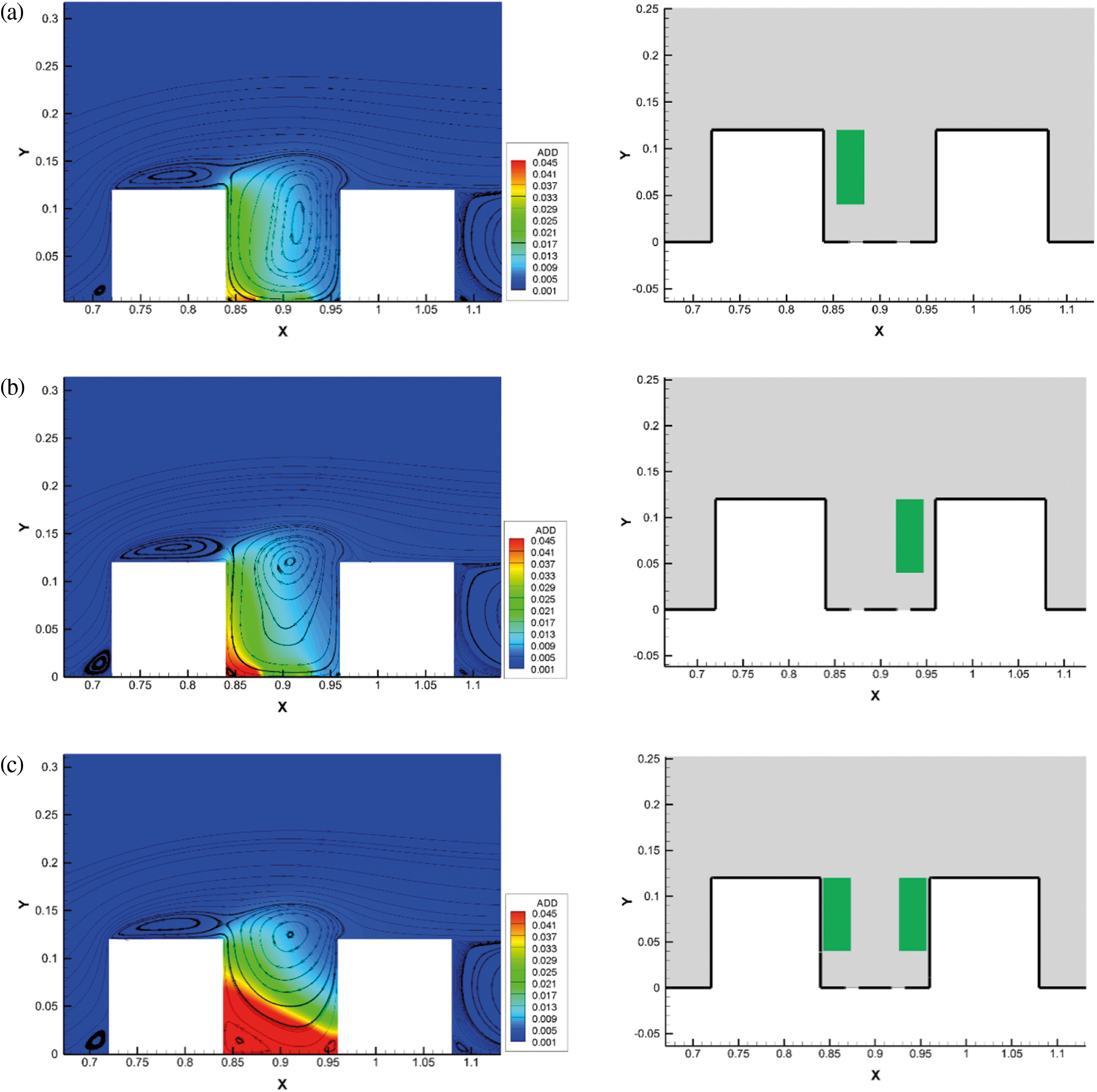
Figure 4: The short-term average daily exposure dose (ADD) contours and streamlines in the schemes where the green belt was established on the (a) leeward, (b) windward, and (c) both sides of the road in turn, with a street canyon aspect ratio (AR) of 1
3.1 Verification of the Simulation and Wind Tunnel Experiment Results
The dimensionless concentrations on the leeward and windward sides of the simulation results were compared with the results of wind tunnel experiments in Table 1. In the wind tunnel, when Y = 0, the standard deviation was 0.133 at the windward side and 9.636 at the leeward side. The results were slightly different, but the overall trends were the same. The dimensionless concentration value on the leeward side was obviously higher than that on the windward side, and it decreased gradually with increasing building height, but there was little change with height on the windward side.
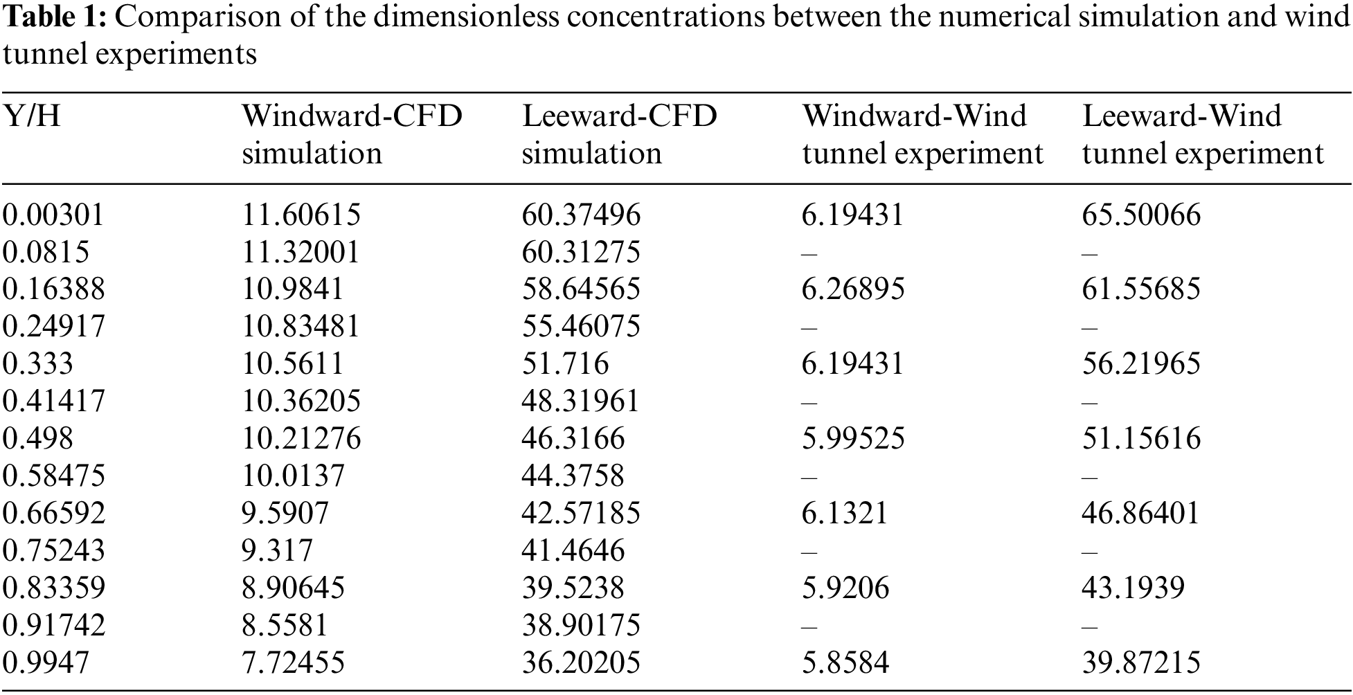
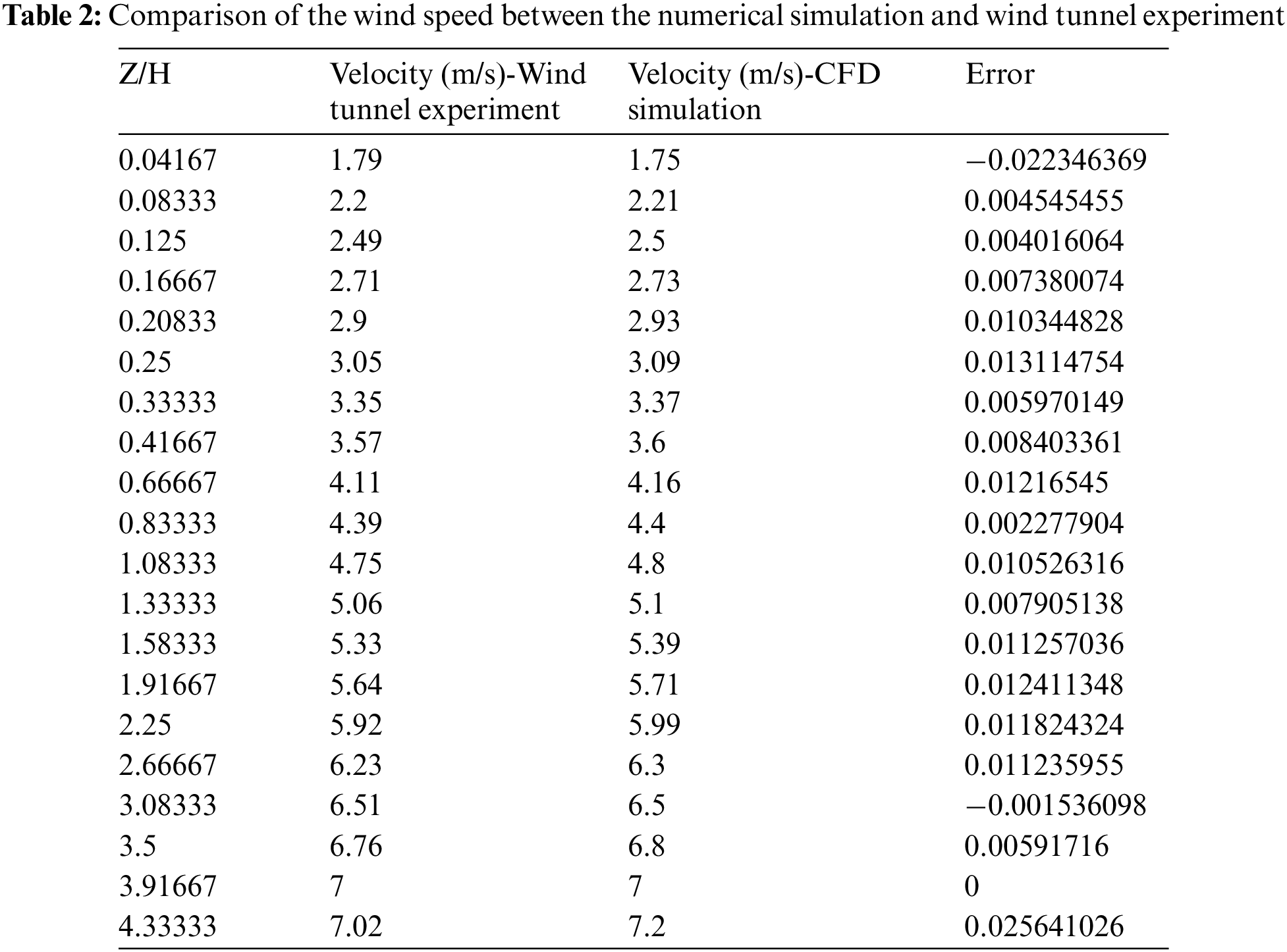
Table 2 shows the velocity inlet boundary surface, and a numerical comparison of the simulated and experimental wind speeds. It can be seen from the figure that the simulated value was in good agreement with the experimental value.
3.2 Comparison of the Simulated Particulate Concentration with Field Measurements
There are few relevant particulate matter wind tunnel experiments that we could use to fit and verify the particulate matter distribution in a street canyon. Therefore, streets with a similar vertical wind direction and wind speed in Jinan were selected for particulate matter measurement. The measured particle concentration was compared with the simulated results.
Field measurements of the PM2.5 concentration were made in a six-story building on the windward side of Qianfoshan Road in Jinan (Fig. 5) where there are two-way four lanes and a green belt on both sides from 9:10–10:30 and 16:30–17:40 (i.e., the morning and evening traffic peaks, respectively) on January 16–18, 2021. Field measurements were conducted with a handheld portable particle counter (model CW-HAT200, M&A Instruments Inc., Arcadia, CA, USA). Data were collected at the windows of corridors on each floor of street-facing buildings, and the recorded values were projected to extend to outside the windows. At least three measurements were taken at each point during each period of the day. During the measurements, the ambient air quality was classified as “good” or “moderate”, which meant that the PM2.5 concentration in the ambient air was in the range of 50–200 μg/m3. The wind direction was approximately perpendicular to the building. There was a consistent gentle breeze during the measurements.
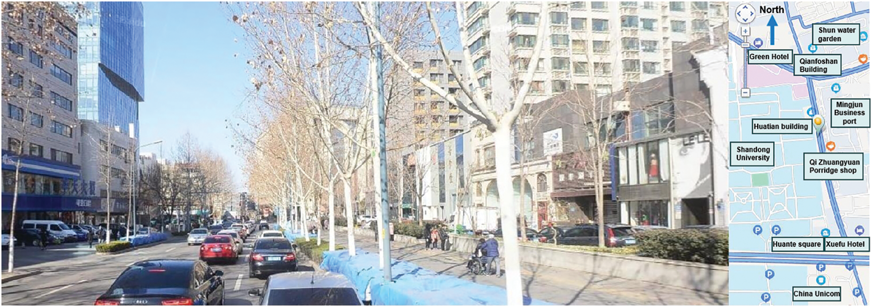
Figure 5: Photographs of the study site
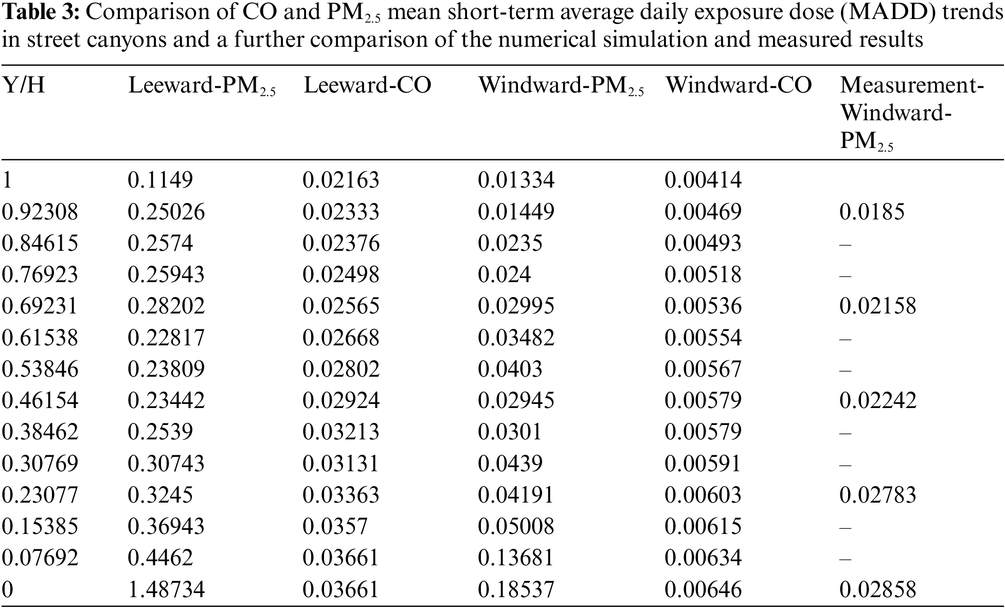
To calculate particle diffusion in street canyons, we numerically simulated the diffusion of PM2.5 in a street canyon with a roadside green belt on both sides, and converted it into a short-term exposure dose for comparison and verification with the measured values. As shown in Table 3, the measured results agreed well with the simulation, with a maximum particle size of 2.5 μm, with only a slight difference in the concentration at ground level. The measured results might have been affected by pedestrian and vehicle activity between the windward side of the building surface and the point of exhaust emissions.
3.3.1 Effects of Canopy Height on Pollutant Dispersion in the Street Canyon
According to the flow field shown in Fig. 2, when the height of the tree canopy was varied in the street canyon there was always a clockwise large vortex that formed, which was consistent withthe results of other similar studies [3,32–36]. However, with the increasing height of the tree canopy, the vortex center tended to shift to the upper right. This was because the green belt was located in the center of the street canyon, which corresponded to the vicinity of the vortex center in the flow field, and the overall intensity of the flow was weak. With an increase in canopy height, the blocking and dragging effect of the canopy on the air flow field was enhanced, resulting in a gradual weakening of the intensity of the air flow in the street canyon. When the height of the tree canopy exceeded the building height, it became difficult for the vortex to enter the street canyon.
The weaker the flow, the more obvious the pollutant aggregation was. Previous studies [37,38] have obtained similar results. As can be seen from Fig. 2, when the tree crown height was 14 m, the pollutant concentration at the leeward side increased significantly, and pollutants could accumulate. This phenomenon indicates that when the overall height of the green belt approaches or even exceeds the height of the buildings, there will be a significant increase in pollutant accumulation. Therefore, roadside green belts should not be designed to be higher than the surrounding buildings.
Fig. 6a shows the mean value of ADD on the leeward and windward sides and near the ground in a street canyon with different canopy heights. The ADD was highest on the leeward side, which was similar to the conclusions of previous studies [2,34]. When the height of the tree crown approached or exceeded the height of the buildings, the ADD increased rapidly. There was a gradual downward trend on the windward side. Turbulence intensity was used to express the characteristics of turbulent flow. Fig. 6a also shows the average turbulence intensity at different canopy heights. The turbulence intensity was negatively correlated with the pollutant concentration.
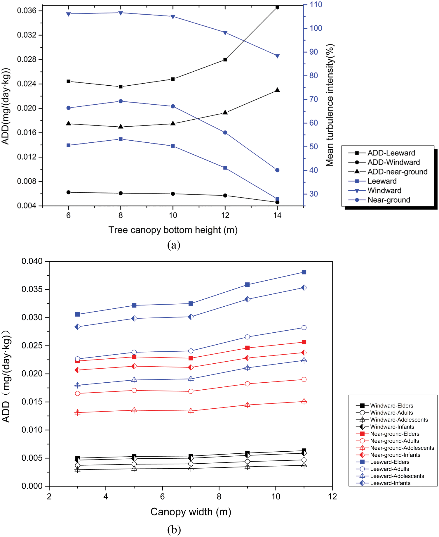
Figure 6: Distribution of mean short-term average daily exposure dose (MADD), turbulence intensity, and velocity on the windward and leeward sides of a street canyon and near the ground. (a) Variation of the short-term average daily exposure dose (ADD) and turbulence intensity in street canyons at different canopy heights (b) Changes in pollutant concentrations and turbulence intensity in street canyons at different canopy heights
3.3.2 Effects of Canopy Width on Pollutant Dispersion in the Street Canyon
As can be seen in Fig. 3, with an increase of canopy width from 3 to 11 m, the vortex center tended to shift to the upper right. This indicates that when the space occupied by the green belt in the street canyon was sufficiently large, air was prevented from entering the street canyon [37,38]. According to the ADD cloud map, when the tree canopy width increased to 9 and 11 m, the pollutant concentration in the leeward side of the street canyon increased significantly. When the canopy width was large, the spatial distance between the canopy boundary and the buildings decreased. This prevented the air flow from entering the downwash channel in the street canyon, and the space occupied by the clockwise vortex flowing out of the street canyon through the upwash channel decreased at the same time. This weakened the intensity of the air flow and aggravated the accumulation of pollutants.
As can be seen from Fig. 6b, when the canopy width exceeded 7 m, its effect on the pollutant concentration increased significantly. To reduce pollutants in a street canyon, the canopy width should be no more than 7 m. The ADD was determined for each age group. The ADD of the elderly and infants was higher than that of the other age groups, which was consistent with the age group distribution of ozone exposure reported by Yang et al. [22]. Therefore, for the elderly and infants, it is recommended to avoid traveling in the peak traffic periods. For residents of street-facing buildings on the leeward side and near the ground, windows should be closed as often as possible during these periods.
3.3.3 Influence of Green Belt Layout and the Street Canyon AR on Pollutant Diffusion
As can be seen from Fig. 4, when AR = 1 and the roadside green belt was established on the leeward, windward, or both sides of the street canyon, the flow structure in the street canyon was presented as a large clockwise vortex, with different vortex centers. This was consistent with other simulations of the vertical wind direction [39–42]. When the roadside green belt was established on the leeward side, the size of the downwash channel was sufficiently large for the air flowto fully enter the street canyon. The air flow entering the canyon was squeezed by the roadside green belt, forcing the center of the vortex to shift to the windward side of the street canyon. When the green belt was established on the windward or both sides of the street canyon, the center of the flow field vortex gradually shifted away from the street canyon. This was because the downwash channel of the flow field was hindered by the roadside green belt, and when the green belt was established on both sides of the road, there was a double resistance to the flow in the street canyon. The intensity of the flow was therefore greatly weakened, and it was difficult for the air flow to fully enter the street canyon.
According to Fig. 4, the different layouts of green belts had little influence on the ADD at building heights, but had a more significant influence on the leeward side and near the ground than on the windward side. When the roadside green belt was distributed on the leeward side and in the center of the street canyon (see Fig. 3c), there was no significant impact on the pollutant concentration. However, when the green belt was established on the windward or both sides, the ADD at the bottom of the leeward side of the street canyon increased significantly. This was consistent with the flow structure. When the green belt was established on both sides of the street canyon, the air flow was subject to the greatest resistance, and the flow intensity in the street canyon was weakest, leading to a large pollutant concentration.
3.3.4 The Diffusion of Particulate Matter in the Street Canyon
Figs. 7a to 7c show the flow and ADD when the green belt was established in the center of the road, compared with no green belt and green belts on both sides. Compared with the flow field for gaseous pollutant diffusion (see Fig. 3c), there was a small counterclockwise vortex at the leeward side of the street canyon, resulting in an accumulation of loosely aggregated particles. The particulate matter concentration was large on the leeward side, especially near the ground, which was consistent with the distribution of gaseous pollutants, and agreed with the results of other particulate matter studies [43,44]. Compared with the flow field diagram for the situation without a green belt, the air flow with a green belt on both sides of the road could not fully enter the canyon, and the intensity of the flow in the street canyon was weakened [18,44]. Compared with the situation without a green belt, the particulate matter concentration with a green belt on both sides of the road was significantly higher, and a large amount of particulate matter was deposited on the ground, which corresponded to the structure and intensity of the flow field.
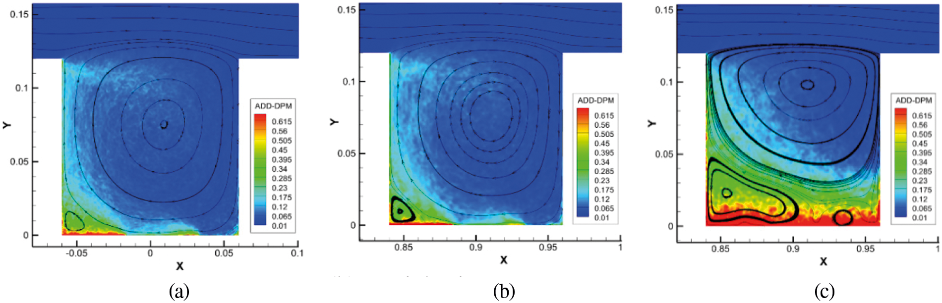
Figure 7: Distribution of short-term average daily exposure dose (ADD) in a street canyon of particle size = 2.5 μm for different wind speeds. (a) Particle size = 2.5 μm; gentle breeze; central green belt (b) Particle size = 2.5 μm; gentle breeze; no green belt (c) Particle size = 2.5 μm; gentle breeze; green belt on both sides
The coordinate of particle size 0 μm in Fig. 8 corresponds to a wind speed without any particulate matter present. By comparing the wind speed without particles and the wind speeds with the six particle sizes, it can be seen that when the wind was less than a gentle breeze, the average wind speeds were smallest for 2.5 and 10 μm particles, and it was therefore not easy for these particles to be dispersed effectively. When the wind speed increased to a moderate breeze and the particle size was larger than 1 μm, the wind speed did not change much, which represented a concentration distribution law, in which a negative correlation was presented between the wind speed and particle concentration. The greater the wind speed, the more conducive it was to the diffusion of particulate pollutants, and the weakening effect of the diffusion of particulate matter on the kinetic energy of the air flow became less significant.
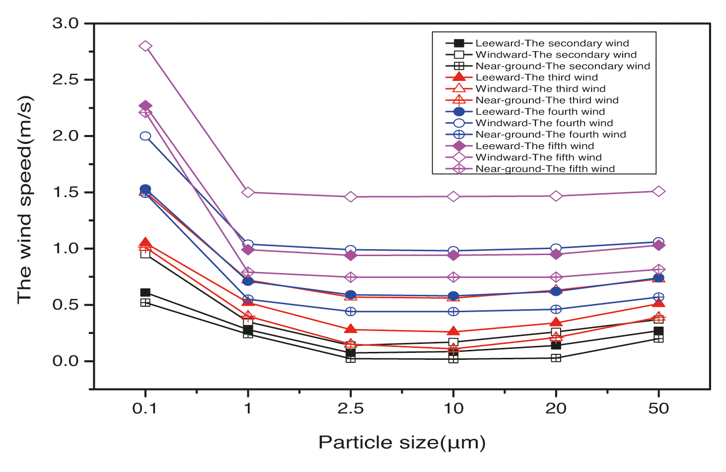
Figure 8: The average wind speed for different particle sizes in street canyons at different wind speeds
Through numerical simulation, the effects of roadside green belts, urban street spatial layout, and wind speed on vehicle exhaust emission diffusion in a street canyon were studied. The diffusion of different sized particles in the street canyon and the influence of wind speed were investigated. Pollutant levels increased with increasing canopy height, canopy width, and decreasing tree spacing, with optimal values of 12 m, 7 m, and 0.4 H, respectively. Central and leeward green belts were most conducive to the diffusion of pollutants, while the layout of the green belts on both sides of the road was the least conducive to the diffusion of pollutants. The individual daily average pollutant intake was used to evaluate the exposure level in the street canyon microenvironment. The results can be used to effectively improve the air quality in street microenvironments and should be considered when renovating old street buildings. The results can also be used to provide protection from pollution for low-rise residents and pedestrians.
In this study, we ignored the effects of solar radiation and different wind directions, and we did not consider the deposition of particles in the analysis of particulate matter. Different types of street canyons in different climates and the use of different vegetation species, with different pollutant uptake rates or particle deposition characteristics in roadside green belts should be considered in future studies.
Acknowledgement: The scientific calculations in this study were done on the HPC Cloud Platform of Shandong University.
Funding Statement: This study was funded by the National Natural Science Foundation of China [Grant No. 11372166] and “Double First-Class” Foundation for the Talents of Shandong University [No. 31380089963090].
Conflicts of Interest: The authors declare that they have no conflicts of interest to report regarding the present study.
1. United Nations Population Programme (2020). https://www.un.org/zh/global-issues/population. [Google Scholar]
2. Wu, W., Jin, J., Carlsten, C. (2017). Inflammatory health effects of indoor and outdoor particulate matter. Journal of Allergy and Clinical Immunology, 141(3), 833–844. DOI 10.1016/j.jac.2018.01.014. [Google Scholar] [CrossRef]
3. Mohammad, H. D., Philip, K. H., Farzaneh, B. A., Ali, A. M., Mahmood, Y. (2020). The effect of the decreasing level of Urmia Lake on particulate matter trends and attributed health effects in Tabriz, Iran. Microchemical Journal, 153, 104434. DOI 10.1016/j.microc.2019.104434. [Google Scholar] [CrossRef]
4. Savannah, M. M., Amy, K. M., Kent, E. P. (2020). Respiratory health effects of exposure to ambient particulate matter and bioaerosols. Comprehensive Physiology, 10(1), 1–20. DOI 10.1002/cphy.c180040. [Google Scholar] [CrossRef]
5. Luan, Y. G., Sun, H. O. (2011). Effect of blade numbers on pressure drop of axial cyclone separators by CFD. Applied Mechanics and Materials, (55–57), 343–347. DOI 10.4028/www.scientific.net/amm.55-57.343. [Google Scholar] [CrossRef]
6. Lu, W., Wang, X., Wang, W., Leung, A. Y. T., Yuen, K. (2002). A preliminary study of ozone trend and its impact on environment in Hong Kong. Environment Internal, 28, 503–512. DOI 10.1016/s0160-4120(02)00078-8. [Google Scholar] [CrossRef]
7. Jin, S., Guo, J., Wheeler, S., Kan, L., Che, S. (2014). Evaluation of impacts of trees on PM2.5 dispersion in urban streets. Atmospheric Environment, 277–287. DOI 10.1016/j.atmosenv.2014.10.002. [Google Scholar] [CrossRef]
8. He, Y., Gu, Z., Lu, W., Zhang, L., Okuda, T. et al. (2019). Atmospheric humidity and particle charging state on agglomeration of aerosol particles. Atmospheric Environment, 197, 141–149. DOI 10.1016/j.atmosenv.2018.10.035. [Google Scholar] [CrossRef]
9. Scungio, M., Stabile, L., Rizza, V., Pacitto, A., Russi, A. et al. (2018). Lung cancer risk assessment due to traffic-generated particles exposurein urban street canyons: A numerical modelling approach. Science of the Total Environment, 631–632, 1109–1116. DOI 10.1016/j.scitotenv.2018.03.093. [Google Scholar] [CrossRef]
10. Gromke, C., Blocken, B. (2015). Influence of avenue-trees on air quality at the urban neighborhood scale. Part I: Quality assurance studies and turbulent schmidt number analysis for RANS CFD simulations. Environmental Pollution, 196, 214–223. DOI 10.1016/j.envpol.2014.10.016. [Google Scholar] [CrossRef]
11. Gromke, C., Blocken, B. (2015). Influence of avenue-trees on air quality at the urban neighborhood scale. Part II: Traffic pollutant concentrations at pedestrian level. Environmental Pollution, 196, 176–184. DOI 10.1016/j.envpol.2014.10.015. [Google Scholar] [CrossRef]
12. Abhijith, K. V., Kumar, P., Gallagher, J., McNabola, A., Baldauf, R. et al. (2017). Air pollution abatement performances of green infrastructure in open road and built-up street canyon environments--A review. Atmospheric Environment, 162, 71–86. DOI 10.1016/j.atmosenv.2017.05.014. [Google Scholar] [CrossRef]
13. Jeanjean, A., Buccolieri, R., Eddy, J., Monks, P., Leigh, R. (2017). Air quality affected by trees in real street canyons: The case of marylebone neighbourhood in central London. Urban Forestry & Urban Greening, 22, 41–53. DOI 10.1016/j.ufug.2017.01.009. [Google Scholar] [CrossRef]
14. Hang, J., Chen, X., Chen, G., Chen, T., Lin, Y. et al. (2020). The influence of aspect ratios and wall heating conditions on flow and passive pollutant exposure in 2D typical street canyons. Building and Environment, 168, 106536. DOI 10.1016/j.buildenv.2019.106536. [Google Scholar] [CrossRef]
15. Kumar, P., Druckman, A., Gallagher, J., Gatersleben, B., Allison, S. et al. (2019). The nexus between air pollution, green infrastructure and human health. Environment International, 133, 105181. DOI 10.4324/9781315064451-20. [Google Scholar] [CrossRef]
16. Riccardo, B., Salim Mohamed, S., Laura Sandra, L., di Silvana, S., Andrew, C. et al. (2011). Analysis of local scale treeeatmosphere interaction on pollutant concentration in idealized street canyons and application to a real urban junction. Atmospheric Environment, 45, 1702–1713. DOI 10.1016/j.atmosenv.2010.12.058. [Google Scholar] [CrossRef]
17. Mamatha, T., Prashant, K., Yendle, B., Pascal, P., Hugh, F. et al. (2021). Green infrastructure for air quality improvement in street canyons. Environment Internal, 146, 106288. DOI 10.1016/j.envint.2020.106288. [Google Scholar] [CrossRef]
18. Wang, X., Lu, W., Wang, W., Leung, A. Y. T. (2003). A study of ozone variation trend within area of affecting human health in Hong Kong. Chemosphere, 52, 1405–1410. DOI 10.1016/s0045-6535(03)00476-4. [Google Scholar] [CrossRef]
19. Wania, A., Bruse, M., Blond, N., Weber, C. (2012). Analysing the influence of different street vegetation on traffic-induced particle dispersion using microscale simulations. Journal of Environmental Management, 94(1), 91–101. DOI 10.1016/j.jenvman.2011.06.036. [Google Scholar] [CrossRef]
20. Xu, W. J., Xing, H., Yu, Z. (2012). Effect of Greenbelt on pollutant dispersion in street canyon. Journal of Environmental Sciences, 33(2), 532–538. DOI 10.5353/th_b3774249. [Google Scholar] [CrossRef]
21. Zhu, X., Lei, L., Han, J., Wang, P., Liang, F. et al. (2020). Passenger comfort and ozone pollution exposure in an air-conditioned bus microenvironment. Environmental Monitoring & Assessment, 192(8), 496. DOI 10.1007/s10661-020-08471-3. [Google Scholar] [CrossRef]
22. Yang, C., Yang, H., Guo, S., Wang, Z., Xu, X. et al. (2012). Alternative ozone metrics and daily mortality in suzhou: The China air pollution and health effects study (CAPES). Science of the Total Environment, 426, 83–89. DOI 10.1016/j.scitotenv.2012.03.036. [Google Scholar] [CrossRef]
23. Pagalan, L., Bickford, C., Weikum, W., Lanphear, B., Brauer, M. et al. (2019). Association of prenatal exposure to air pollution with autism spectrum disorder. JAMA Pediatrics, 173, 86–92. DOI 10.5353/th_b5098886. [Google Scholar] [CrossRef]
24. Sallis, J. F., Haskell, W. L., Wood, P. D., Fortmann, S. P., Rogers, T. et al. (1985). Physical activity assessment methodology in the five-city project. American Journal of Epidemiology, 121(1), 91. DOI 10.1093/oxfordjournals.aje.a113987. [Google Scholar] [CrossRef]
25. Zou, B., Wilson, J. G., Zhan, F. B., Zeng, Y. (2009). Air pollution exposure assessment methods utilized in epidemiological studies. Journal of Environmental Monitoring, 11, 475–490. DOI 10.1039/b813889c. [Google Scholar] [CrossRef]
26. Buccolieri, R., Gromke, C., Sabatino, S. D., Ruck, B. (2009). Aerodynamic effects of trees on pollutant concentration in street canyons. Science of the Total Environment, 407(19), 5247–5256. DOI 10.1016/j.scitotenv.2009.06.016. [Google Scholar] [CrossRef]
27. Oke, T. R. (1988). Street design and urban canopy layer climate. Energy and Buildings, 11(1–3), 103–113. DOI 10.1016/0378-7788(88)90026-6. [Google Scholar] [CrossRef]
28. Fluent a. 12.0 User's guide (2009). User Inputs for Porous Media. [Google Scholar]
29. Huang, H., Akutsu, Y., Arai, M., Tamura, M. (2000). A two-dimensional air quality model in an urban street canyon: Evaluation and sensitivity analysis. Atmospheric Environment, 34(5), 689–698. [Google Scholar]
30. Hunter, L. J., Watson, I., Johnson, G. (1991). Modelling air flow regimes in urban canyons. Energy and Buildings, 15(3), 315–324. DOI 10.1016/0378-7788(90)90004-3. [Google Scholar] [CrossRef]
31. Zhong, J., Cai, X., Bloss, W. J. (2016). Coupling dynamics and chemistry in the air pollution modelling of street canyons: A review. Environmental Pollution, 214, 690–704. DOI 10.1016/j.envpol.2016.04.05. [Google Scholar] [CrossRef]
32. Huang, Y., Lin, X., Zhao, S. (2013). Numerical simulation on dispersion and deposition of particles within a street canyon. Journal of University of Shanghai for Science and Technology, 35(1), 51–54. DOI 10.5353/th_b4660703. [Google Scholar] [CrossRef]
33. Xie, X., Huang, Z., Wang, J. S. (2005). Impact of building configuration on air quality in street canyon. Atmospheric Environment, 39, 4519–4530. DOI 10.1016/j.atmosenv.2005.03.043. [Google Scholar] [CrossRef]
34. Xie, X., Huang, Z., Wang, J., Xie, Z. (2005). The impact of solar radiation and street layout on pollutant dispersion in street canyon. Building and Environment, 40, 201–212. DOI 10.1016/s0140-6701(05)80940-3. [Google Scholar] [CrossRef]
35. Gromke, C., Buccolieri, R., Sabatino, S. D., Ruck, B. (2008). Dispersion study in a street canyon with tree planting by means of wind tunnel and numerical investigations–evaluation of CFD data with experimental data. Atmospheric Environment, 42, 8640–8650. DOI 10.1016/j.atmosenv.2008.08.019. [Google Scholar] [CrossRef]
36. Gallagher, J., Baldauf, R., Fuller, C. H., Kumar, P., Gill, W. L. et al. (2015). Passive methods for improving air quality in the built environment: A review of porous and solid barriers. Atmospheric Environment, 120, 61–70. [Google Scholar]
37. Amorim, J. H., Rodrigues, V., Tavares, R., Valente, J., Borrego, C. (2013). CFD modelling of the aerodynamic effect of trees on urban air pollution dispersion. Science of the Total Environment, 461–462, 541–551. DOI 10.1016/j.scitotenv.2013.05.031. [Google Scholar] [CrossRef]
38. Buccolieri, R., Salim, S. M., Leo, L. S., Sabatino, S. D., Chan, A. et al. (2011). Analysis of local scale tree-atmosphere interaction on pollutant concentration in idealized street canyons and application to a real urban junction. Atmospheric Environment, 45, 1702–1713. DOI 10.1016/j.atmosenv. [Google Scholar] [CrossRef]
39. Huang, Y. D., Hou, R. W., Liu, Z. Y., Song, Y., Cui, P. Y. et al. (2019). Effect of wind direction on the airflow and pollutant dispersion inside a long street canyon.Aerosol and Air Quality Research, 19, 1152–1171. DOI 10.4209/aaqr.2018.09.0344. [Google Scholar] [CrossRef]
40. Bailey, W. G., Oke, T. R., Rouse, W. R. (1997). The surface climates of Canada. Montreal: McGill-Queen's University Press. [Google Scholar]
41. Soulhac, L., Perkins, R. J., Salizzoni, P. (2008). Flow in a street canyon for any external wind direction. Boundary-Layer Meteorology, 126, 365–388. DOI 10.1007/s10546-007-9238-x. [Google Scholar] [CrossRef]
42. Pospisil, J., Jicha, M., Niachou, K., Santamouris, M. (2005). Computational modelling of airflow in urban street canyon and camparison with measurements. International Journal of Environment and Pollution, 25(1), 60–64. DOI 10.1504/ijep.2005.007666. [Google Scholar] [CrossRef]
43. Zhang, L., Zhang, Z., McNulty, S., Wang, P. (2020). The mitigation strategy of automobile generated fine particle pollutants by applying vegetation configuration in a street-canyon. Journal of Cleaner Production, 274, 122941. DOI 10.1016/j.jclepro.2020.122941. [Google Scholar] [CrossRef]
44. Lin, X. L., Chamecki, M., Yu, X. P. (2020). Aerodynamic and deposition effects of street trees on PM2.5 concentration: From street to neighborhood scale. Building and Environment, 185, 107291. DOI 10.1016/j.buildenv.2020.107291. [Google Scholar] [CrossRef]
 | This work is licensed under a Creative Commons Attribution 4.0 International License, which permits unrestricted use, distribution, and reproduction in any medium, provided the original work is properly cited. |