Computer Modeling in Engineering & Sciences

DOI: 10.32604/cmes.2022.020260

ARTICLE

A New Criterion for Defining Inhomogeneous Slope Failure Using the Strength Reduction Method

Chengya Hua1, Leihua Yao1,*, Chenguang Song1, Qihang Ni1 and Dongfang Chen2

1School of Engineering and Technology, China University of Geosciences, Beijing, 100083, China
2Center for Hydrogeology and Environmental Geology, China Geological Survey, Tianjin, 300309, China
*Corresponding Author: Leihua Yao. Email: leihuayao@163.com
Received: 13 November 2021; Accepted: 22 December 2021

1  Introduction

Slope stability is a classic and frequent problem in geotechnical engineering. The stability evaluation of complex inhomogeneous slopes in construction is an important measure to ensure construction safety. The factor of safety (FOS) is often used to evaluate slope stability [1–5]. Scholars have proposed the limit equilibrium method (LEM) for calculating FOSs of slopes. As a kind of LEM, the wedge method is widely used to calculate the FOS of slopes. Zaki et al. [6] discussed the applicability of the generalized wedge method to slope stability analysis in rock engineering. McCombie [7] proposed a slope stability analysis method based on multiple wedges. Rong et al. [8] derived the upper bound solution and classical solution method for the stability of rock wedges. The above research shows the effectiveness of the wedge method in calculating the FOS of slopes. Considering the complex soil layer and geometry of a three-dimensional heterogeneous slope, a simplified three-dimensional limit equilibrium method (STLEM) learning from the wedge method is proposed to calculate the FOS of the slope in this paper.

In addition to the LEM, the strength reduction method is used to calculate the FOS of the slope. The FOS of slope was calculated, and the failure mechanism was analyzed using the SRM [9]. Using the SRM, Jiang et al. [10] simulated the deformation of the slope block of a hydropower station. Tu et al. [11] analyzed the FOS of a slope with a variable slope gradient based on the SRM. Wei et al. [12] used SRM and LEM to calculate the FOS of the slope and concluded that the calculation results of the two methods were consistent. The LEM and SRM are widely used in slope stability analysis. The SRM is convenient and efficient, especially for complex inhomogeneous slopes, as it does not require the assumption of a slippery surface. Relevant scholars have indicated that this method is consistent with LEM in terms of feasibility and reliability in application. For SRM, the FOS of the slope depends on the selected instability criterion. At present, there are four general instability criteria: (1) displacement mutation (criterion I), that is, the strength reduction coefficient corresponding to the displacement curve mutation point at the monitoring point is FOS [13,14]. (2) Plastic zone penetration (criterion II), that is, when there is a plastic band through the model to form a plastic flow condition, the corresponding strength reduction coefficient is FOS [15,16]. (3) Calculation nonconvergence (criterion III), that is, when the calculation program of the model does not converge, the corresponding strength reduction coefficient is FOS [17]. (4) Energy mutation (criterion IV), that is, the strength reduction coefficient corresponding to the mutation point of the energy curve of the model, is FOS [11,18]. Because of the importance of criteria, relevant scholars have conducted extensive discussions on these criteria. Using a two-dimensional slope example, Li et al. [19] concluded that the FOS determined by criterion I was consistent with that determined by criterion II. Yang et al. [20] analyzed a two-dimensional slope and found that the FOSs obtained by criterion I and criterion II were closer to the Spenser limit equilibrium method. Tu et al. [11] proposed criterion IV and verified that the criterion was consistent with other general criteria (criterion I, criterion II, and criterion III) through several two-dimensional slopes and a three-dimensional slope. In summary, criterion I considers the zone strain of the model, criterion II considers the zone stress of the model, criterion III considers the numerical algorithm of the calculation, and criterion IV considers the zone stress and strain of the model. However, the four criteria have their own disadvantages. Criterion I takes a large amount of work to select monitoring points and displacement directions when analyzing structures with unclear failure mechanisms. For criterion II, there is no clear standard for the penetration of plastic zones, and it is difficult to determine the standard for a structure with unclear failure mechanisms. For criterion III, convergence is limited by the numerical algorithm, and there is human error in setting the convergence standard. For criterion IV, the mutation of the curve between the energy and the strength reduction factor requires human judgment and lacks mechanical explanation. These four criteria have some common shortcomings. For example, instability is only determined by the local physical quantity of the model, there is human error in the judgment of the instability, and there is a lack of rigorous mechanical derivation and demonstration.

The variational method is classic in geotechnical engineering and is often used to analyze slope stability [21]. Leshchinsky et al. [22] applied the variational method to analyze the stability of a three-dimensional slope. Jiang et al. [23] compared the variational method with a three-dimensional critical sliding surface search method. Einav [24] analyzed piles using the variational method and energy principle. Navarro et al. [25] used the variational method for the sensitivity analysis and determination of the critical slip surface. Nie et al. [26] analyzed the slope stability by transforming the problem of the contact between the sliding body and the sliding bed into a variational problem. The above studies show that the variational method is widely used in the field of slope stability. However, it has not been used in combination with the SRM to judge slope instability. To overcome the shortcomings of the above four criteria, a variational method combined with SRM is proposed.

In this paper, the variational method is used to derive the variational calculation formula of the numerical models. Then, by means of FLAC3D software and the built-in FISH language, the variational calculation program is written. In the end, the variational value of the model is calculated, and the stability of the model is transformed into the judgment of the positive or negative value. With a definite objective index, this method provides a strict mechanical basis for evaluating slope stability and avoids human error. First, the basic theory of the SRM and the variational method are introduced. Then, based on the classical two-dimensional and actual three-dimensional examples, the corresponding numerical models are established. Based on the numerical models, the four general criteria, the variational method, and STLEM are used to calculate the FOSs of the slope. Then, the FOSs calculated by the criteria and methods are discussed. Finally, conclusions are drawn.

2  Theory

2.1 Strength Reduction Method

The basic principle of SRM is as follows. The initial strength parameters are substituted into the model for calculation. When the model is stable, the initial strength parameter is divided by the strength reduction factor. After division, the new parameters are substituted into the model for the second calculation. Among the above, the initial strength reduction coefficient is 1.00, and the coefficient increases by 0.01 at one time. The strength reduction coefficient is determined as the FOS of the model when it is unstable. As shown in Eq. (1), the initial strength parameters c,φ are divided by the strength reduction coefficient k to obtain the new strength parameters c′,φ′.

c′=c/kφ′=tan−1⁡(tanφ/k)(1)

2.2 Criterion I

Several key points in the model are selected to monitor the displacement of the monitoring point under each strength reduction factor. The relation curve between the displacement and the strength reduction factor is drawn. The strength reduction factor corresponding to the mutation point of the curve is taken as the FOS of the model.

2.3 Criterion II

The shear strain increment cloud images under different strength reduction coefficients of the model are observed. The strength reduction factor of the previous step is taken as the FOS of the model when the plastic band is formed through the model.

2.4 Criterion III

The FOS can be obtained by the nonconvergence of the calculation program. FLAC3D is a finite-difference software with the built-in convergence standard. The FOS command inside can give the FOS of the slope. This criterion takes the value given by the FOS command as the FOS of the slope.

2.5 Criterion IV

It is a trend to take strain energy as a characterization of model stability. This criterion monitors the elastic and plastic strain energies of the model under different strength reduction coefficients. The reduction coefficient corresponding to the abrupt change point of the curve between the plastic strain energy and the strength reduction coefficient is taken as the FOS of the model. The reduction factor corresponding to the maximum point of the curve between the elastic strain energy and the strength reduction factor is taken as the FOS of the model.

2.6 Variational Method

The total potential energy (Et) is an important index to measure the stability of the model. Whether the model is stable or not, the Et of the model remains unchanged when there is a small variation that satisfies the boundary condition because the external and internal forces of the model are in equilibrium, and the work done by the internal force (U) and that by the external force (W) cancel each other out. Reflected in mathematical expressions, the first-order variation of Et is always equal to zero. According to the minimum extremum principle, Et is always the minimum when the model is in a stable state. Reflected in the mathematical expression, the second-order variation of Et is greater than zero. The first-order variation of Et is always equal to zero, which means that Et always takes extreme values. When the model is in an unstable state, the minimum value of Et is not taken. Therefore, the maximum value of Et is taken. Reflected in the mathematical expression, the second-order variation of Et is less than zero. Hence, the stability of the system can be determined according to the positive or negative second-order variational values of Et. The relevant formulas are derived as Eqs. (2) and (3).

Et=U−W(2)

δEt=δU−δW=∫[U(εij0+δεij)−U(εij0)]dΩ−{∫[f¯i(ui0+δui)−f¯i(ui0)]dΩ+∫[T¯i(ui0+δui)−T¯i(ui0)]dS}(3)

where U,f¯i,T¯i represent the strain energy of the model, the body force tensor, and the surface force tensor. εij0,ui0 represent the initial strain tensor and displacement tensor, while δεij,δui represent the first-order variations of the strain tensor and displacement tensor. S,Ω represent the area and volume of the model. When the second-order minute quantity is ignored and U,f¯i,T¯i are expanded according to the Taylor series, the first-order variation of Et can be expressed as Eq. (4).

δEt=∫σij0δεijdΩ−[∫f¯i(δui)dΩ+∫T¯i(δui)dS](4)

where σij0 represents the initial stress tensor. For a certain model, f¯i is constant, and the work done by T¯i is zero. Therefore, the formula of the second-order variation of Et is expressed as Eq. (5).

δ2Et=∫δσijδεijdΩ(5)

where δσij is the first-order variation of the stress tensor. The key is to judge whether the variational value is positive or negative, not large or small. To unify the order of the magnitude of the variational values of different numerical models, the variational values calculated by the above formula are divided by the total volume of the model to obtain the average variation. The variational value of the model mentioned below is the average variational value, which can be calculated by Eq. (6).

vv=∫δσijδεijdΩ∫dΩ(6)

The FISH command in FLAC3D software can retrieve the stress and strain of the element. With a certain strength reduction coefficient, the stress and strain of each element are obtained by the FISH language after calculation. Then, the stress and strain of each element are obtained by applying a small deformation in accordance with the boundary conditions. The latter stress and strain of each element are subtracted by the former to obtain the variational value. The stress variation is multiplied by the strain variation and volume to obtain the variation of the element. By accumulating element variation and dividing it by the total volume of the model, the average variation of the model under the strength reduction coefficient is obtained. Finally, the state of the model is determined by variation. If the variational value is positive, the model is stable. If the variational value is negative, the model is unstable.

Calculation Process for the Variational Method

As shown in Fig. 1, the initial value of the strength reduction coefficient is 1.00, and the reduction coefficient increases by 0.01 at each step. The average variational value of each step of the model is calculated according to the variation calculation program. If the variational value is positive, the calculation continues. If the variational value is negative, the strength reduction factor of the previous step is taken as the FOS of the model.

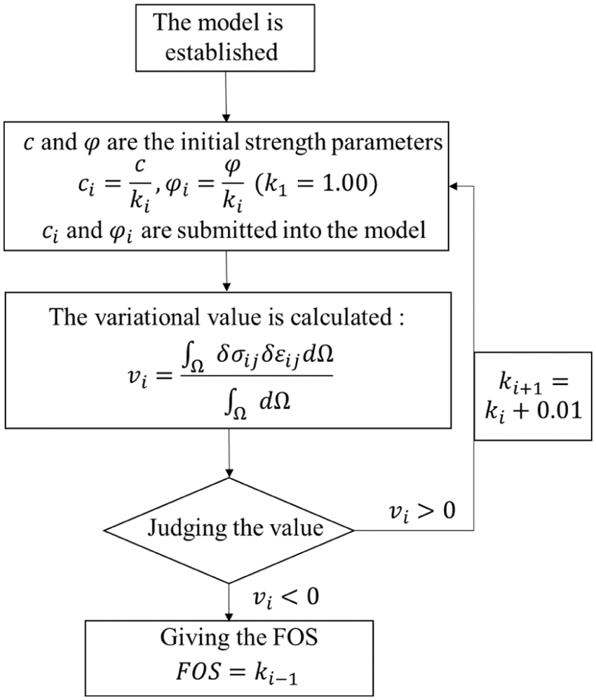
Figure 1: Flow chart of the application of the variational method

3  The Classical Example

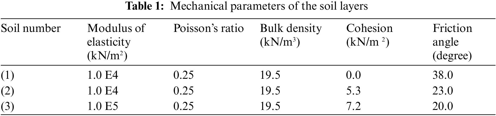
The Australian Computer Aided Design Society (ACADS) provides a classic example of a two-dimensional inhomogeneous slope, which is used in this paper to compare the variational method with other criteria of SRM and international standard answers. The geometric dimensions and soil layers of the example slope are shown in Fig. 2. The ideal elastoplastic constitutive relation and the associated flow rule are adopted for the soil, and the Mohr–Coulomb criterion is adopted for the yield criterion. The relevant key parameters are listed in Table 1.

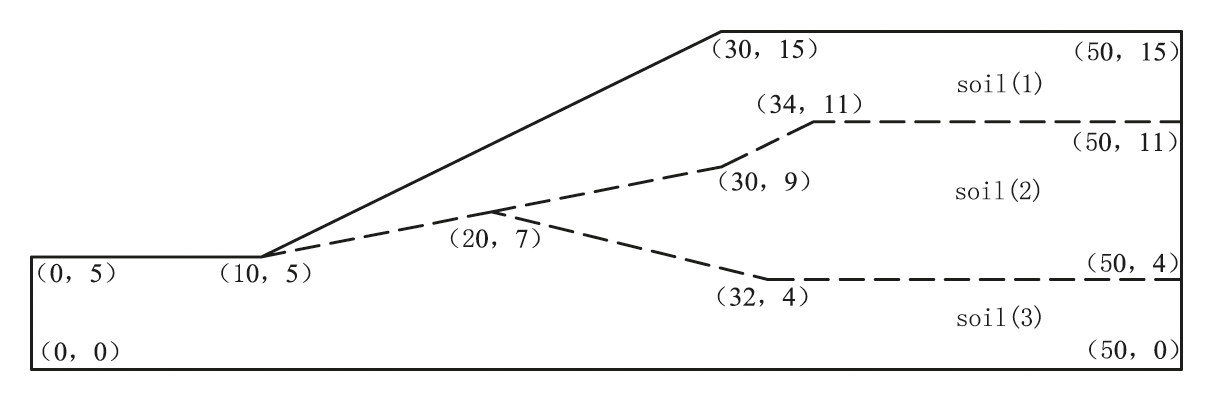
Figure 2: The ACADS example

The numerical model (Fig. 3) is established according to the example, and several nodes are marked. The soil layer numbers are (1), (2), and (3) from top to bottom, respectively. The size of the model is 50 m in the X direction, 0.5 m in the Y direction, and 15 m in the Z direction. The model contains 2160 nodes and 1046 elements. The gradient of the slope is 1:2.

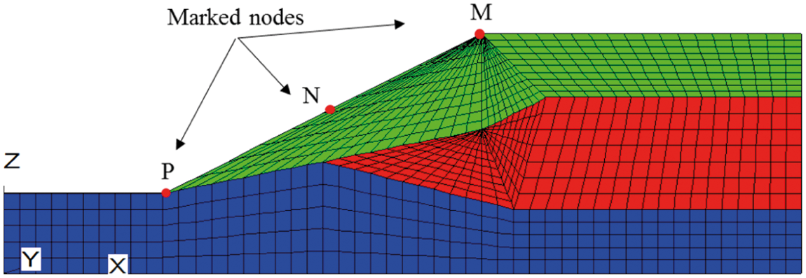
Figure 3: The numerical model of the slope

3.1 Criterion I

A landslide generally refers to a sudden slide of the sliding body on the sliding surface, accompanied by a sudden increase in displacement from top to bottom. Points on the slope (Fig. 3) are taken as the key points for monitoring displacements. The relationship between the displacements and the strength reduction coefficients is shown in Fig. 4.

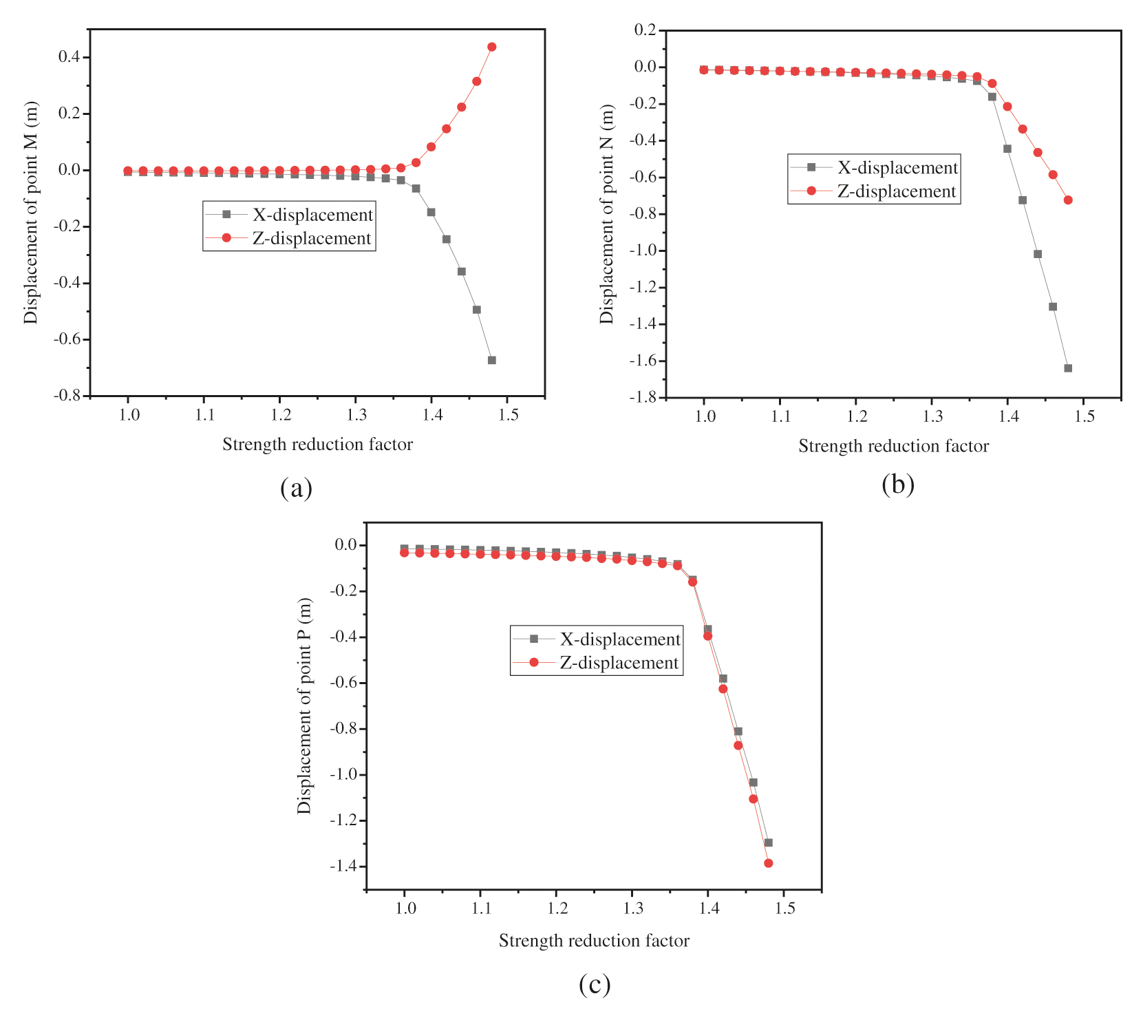
Figure 4: Curves between marked displacements and strength reduction factors

For point M at the top of the slope, there are apparent mutation points in the displacement curves in the X and Z directions. The curves of the two are similar, and there are mutation points in both. The displacement changes slowly when the strength reduction coefficient is between 1.00 and 1.38 but increases rapidly when the strength reduction coefficient is between 1.42 and 1.48, indicating that sliding has taken place. When the strength reduction coefficient is between 1.38 and 1.42, the strength reduction coefficient increases by 0.02, and the displacement increases exponentially, indicating that the model is in a failure state. For point N in the middle of the slope, the shape of the curve is basically the same as that of point M. However, the mutation of the curve is more obvious, and the displacements in the X direction are greater than those in the Z direction. For point P at the bottom of the slope, the displacements in the X and Z directions are close, and both curves have obvious mutation points. This demonstrates that there are mutation points in the displacement curves, where the strength reduction factor is 1.38. According to this criterion, the FOS of the slope is 1.38.

3.2 Criterion II

According to the FISH command, the shear strain increment picture of the model under different strength reduction coefficients can be obtained. As shown in Fig. 5, the plastic zones are not connected, and the slip band is not formed when the strength reduction factor is 1.38, but they are connected to form a penetrating slip band when the strength reduction factor is 1.40. Under landslide conditions, the slope tends to slide. According to the displacement curves, the displacements in the X and Z directions increase suddenly when the strength reduction coefficient is greater than 1.38. The occurrence of landslides revealed by the displacement curves is consistent with the landslide mechanism revealed by the shear strain increment in the model. For safety, the FOS of the slope is determined to be 1.38 according to this criterion.

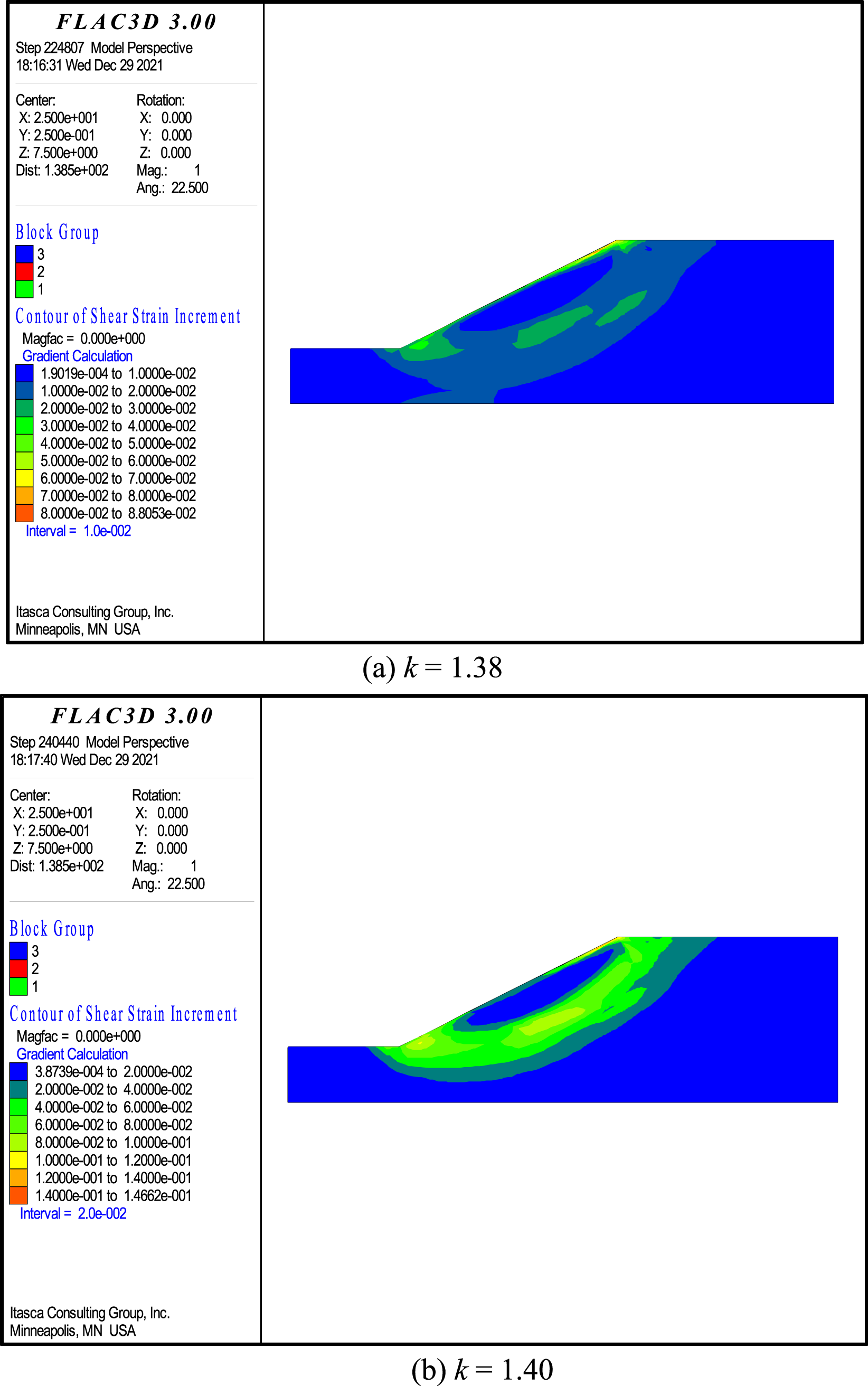
Figure 5: Pictures of shear strain increments when the reduction factor is 1.38 and 1.40 (a) k = 1.38 (b) k = 1.40

3.3 Criterion III

The contours of the plastic zones at the end of the calculation are given in Fig. 6. FLAC3D has a built-in FOS command with a built-in convergence standard. The calculation will end automatically when the model calculation does not converge. The FOS obtained by the FOS command is equivalent to that obtained by criterion III. Therefore, the FOS for this model is confirmed as 1.38 according to this criterion.

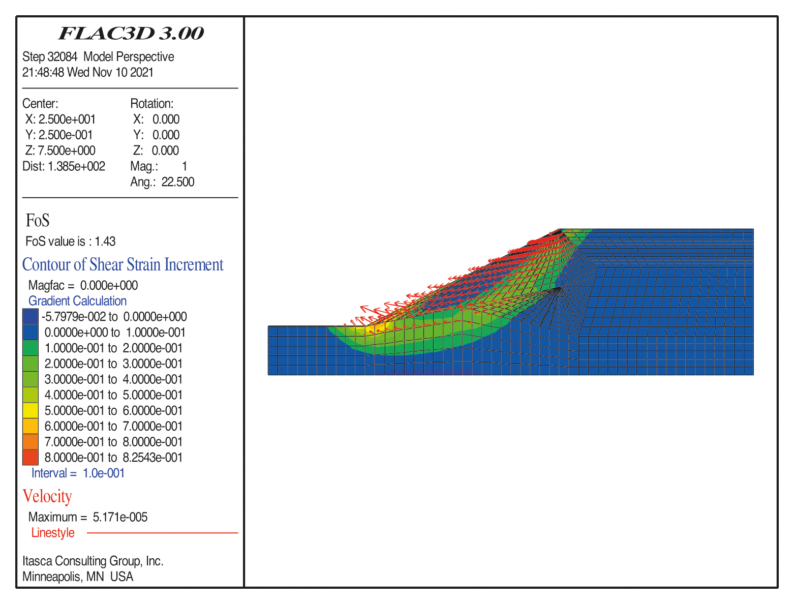
Figure 6: The contour when the calculation program converges (FOS = 1.43)

3.4 Criterion IV

Some researchers proposed and demonstrated the feasibility and accuracy of criterion IV from the principle of energy conservation. With the help of the finite difference software FLAC3D, the command streams for calculating the elastic and plastic strain energy values of the model were programmed. The relationships between the two values and the strength reduction coefficient are analyzed based on inhomogeneous slopes. The FOS of the slope is determined by the mutation of the curves between the energy value and strength reduction coefficient. The strain energy of the slope under each strength reduction coefficient was calculated, as shown in Fig. 7. In terms of plastic strain energy, there are obvious mutation points in the curve. The curve is flat without significant change when the strength reduction factor is less than 1.38 but climbs rapidly when the strength reduction coefficient is between 1.38 and 1.42. When the strength reduction coefficient increases by 0.02, the energy value increases several times, which indicates the occurrence of slope failure. In terms of elastic strain energy, there is a maximum value point in the curve. When the strength reduction factor is less than 1.38, the curve grows slowly. When the strength reduction coefficient is 1.38, the value reaches the maximum. When the strength reduction coefficient is between 1.38 and 1.42, the curve shows a downward trend. According to the above analysis, the slope is unstable when the strength reduction factor is 1.38. Therefore, according to this criterion, the FOS of this model is 1.38.

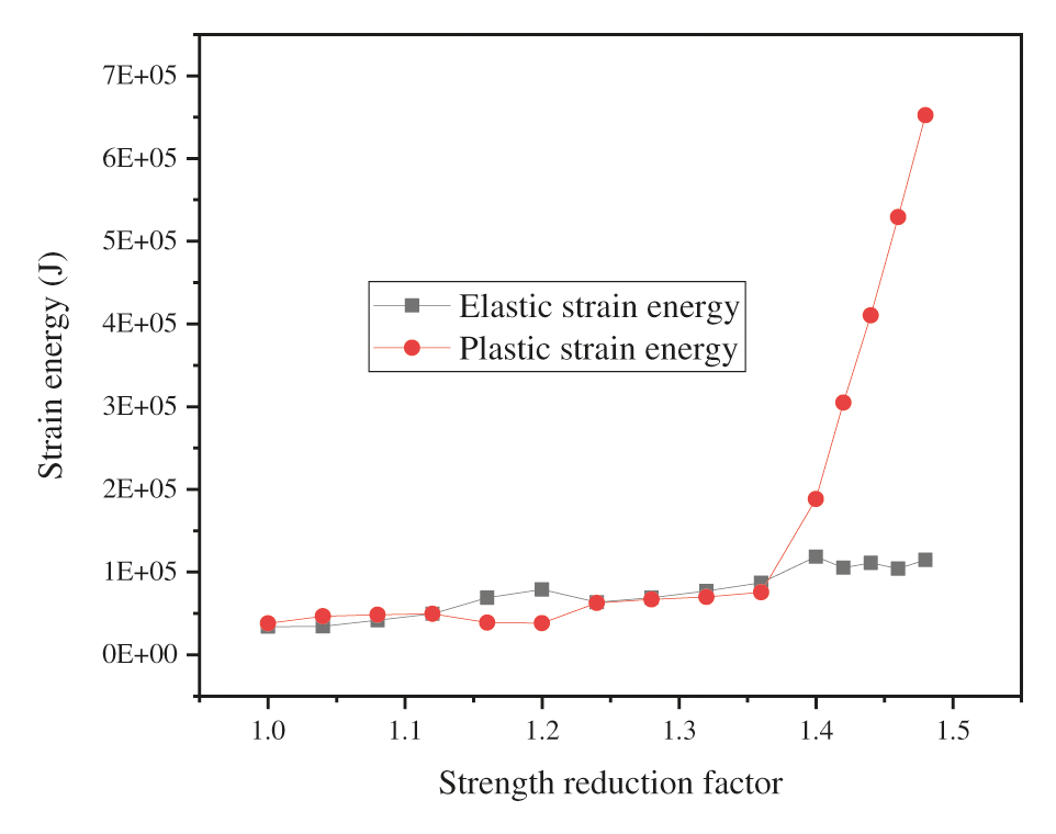
Figure 7: Curves between the strain energy value and strength reduction factor

3.5 Variational Method

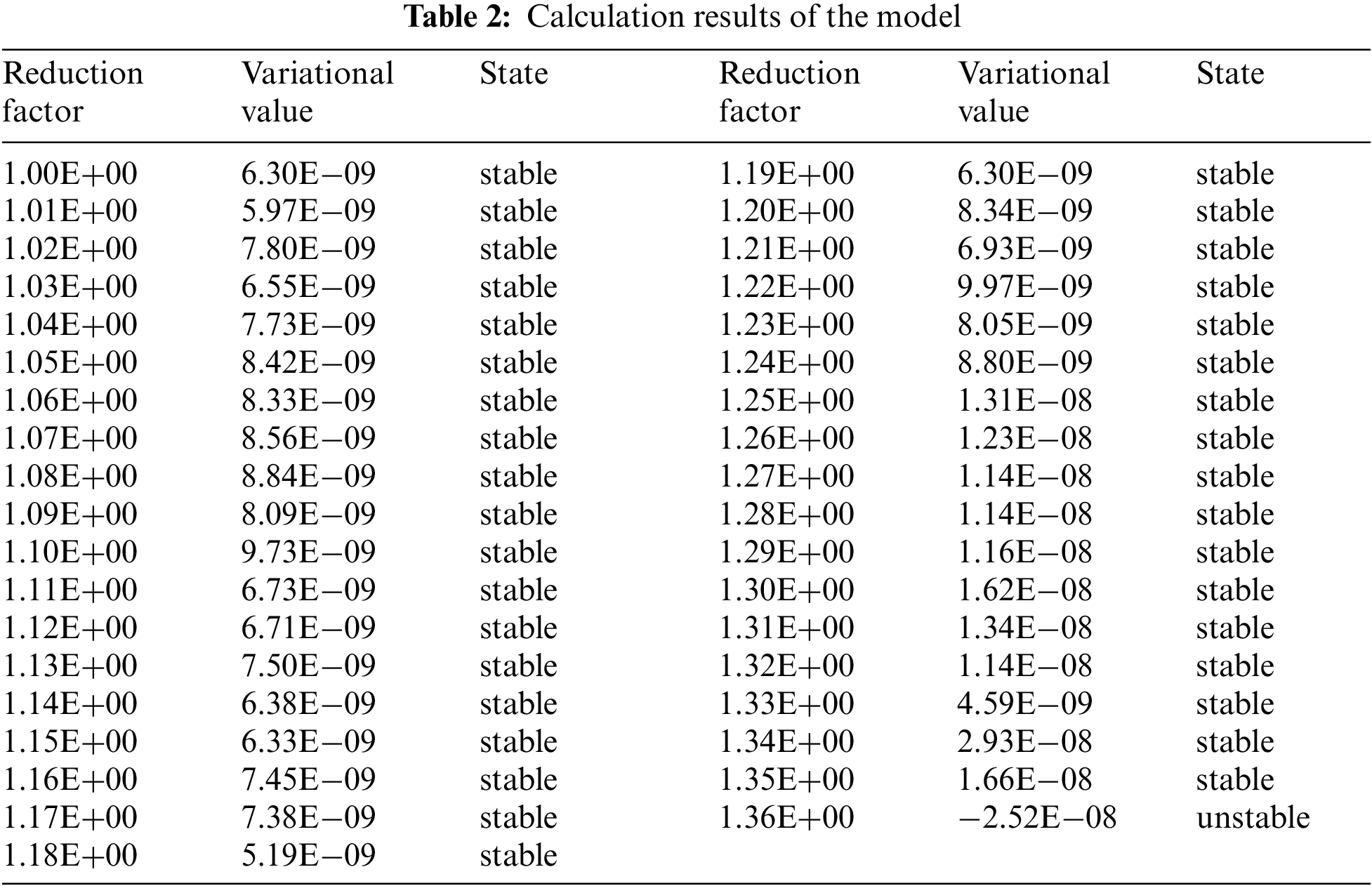
The internal stress and strain of the slope are constantly coupled under the action of force. Most scholars simplify slope stability as the mutation of a single index, namely, the four instability criteria mentioned above. These criteria lack mechanical derivation and cannot reflect the internal mechanism of the slope. Considering the above shortcomings, this paper proposes a variational method for determining slope instability. The results calculated by the variational method are listed in Table 2, which describes the state of the model. The strength reduction coefficient gradually increases from 1.00 to 1.35 with an interval of 0.01. When the strength reduction coefficient is less than or equal to 1.35, the value is positive. When the strength reduction coefficient is 1.36, the value becomes negative for the first time. This result is consistent with the process of plasticity development and failure of the model indicated by other criteria, which suggests that the variational method is feasible. The FOS based on this method is 1.35, which is close to other criteria.

3.6 Contrasts

The relative error D0 between the variational method and other criteria (or methods) is calculated by Eq. (7).

D0=|Fi−F0F0|(7)

where F0,Fi are the FOSs under the variational method, other criteria or methods. The calculation results are listed in Table 3. The left column is the FOS under each criterion or method, and the right column is the corresponding relative error.

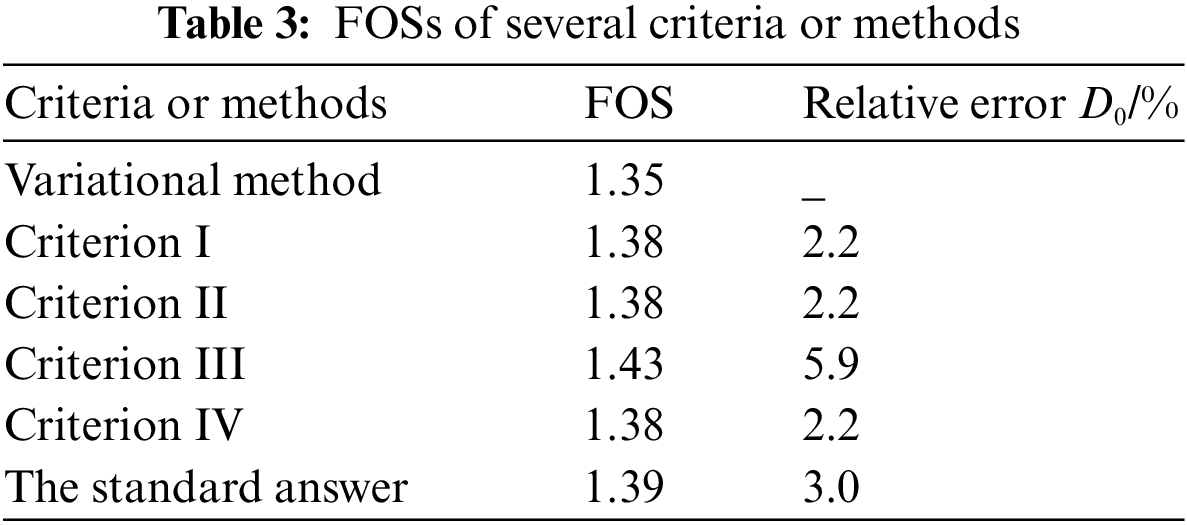
The FOS based on the variational method is close to that of other criteria and standard answers. The FOS obtained by this method is less than those obtained by criterion I, criterion II, and criterion IV, with a relative error of 2.2%. It is also less than those by criterion III and the standard answer with relative errors of 5.9% and 3.0%, respectively. The numerical value and error are small, which reflects the applicability and safety of the variational method. This method consolidates other standards without identifying critical areas of the structure and setting up monitoring points. The method can comprehensively reflect the coupling effect of stress and strain of the structure, which has more advantages than other criteria. In addition, the method has rigorous mathematical and physical derivation, which provides a mechanical explanation for the instability of the model. The variational method is verified to be reliable for two-dimensional inhomogeneous slopes.

4  The Engineering Example

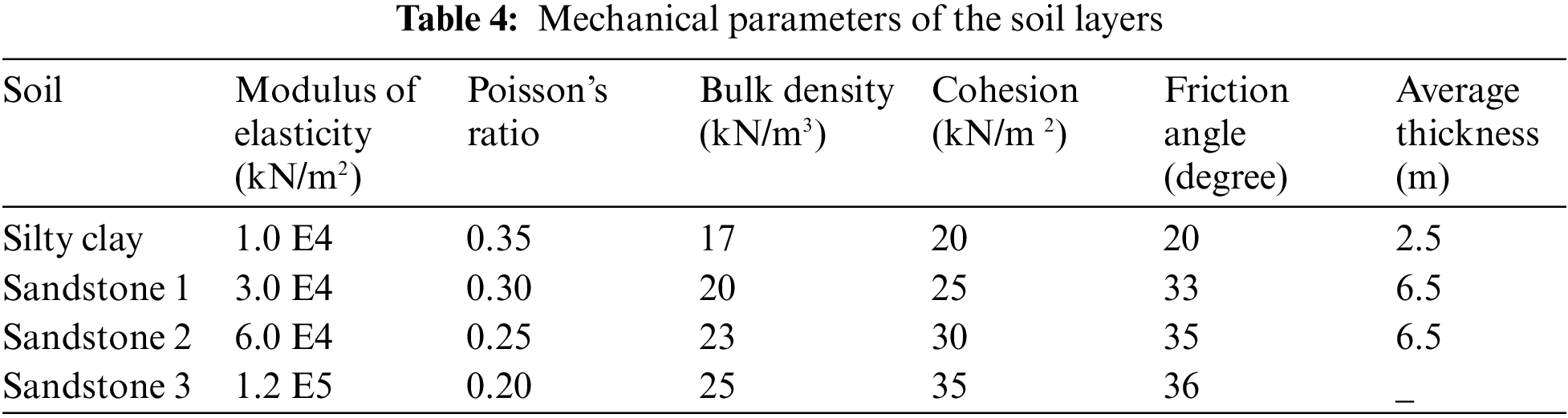
There is a cutting slope on a highway. The elastic modulus is 3–5 times the compression modulus provided in the geological survey report, and other parameters are fine-tuned based on the geological survey report. The ideal elastoplastic constitutive relation and the associated flow rule are adopted for the soil. The Mohr–Coulomb criterion is adopted for the yield criterion. The relevant key parameters are listed in Table 4.

The projection of the slope on the plane Y = 0 is shown in Fig. 8. The projection of the slope on the plane X = 0 is shown in Fig. 9. The numerical model (Fig. 10) is established according to the cutting slope. The soil layer is composed of silty clay, sandstone 1, sandstone 2, and sandstone 3 from top to bottom. The size of the model is 186 meters in the X direction, 130 meters in the Y direction, and 90 meters in the Z direction. The model contains 19,226 nodes and 95,002 elements. The gradient of the slope toward the road is 1:0.75, while the rest is 1:1.00. The slope toward the road is relatively smooth, while that along the road is steep where a landslide is likely to occur.

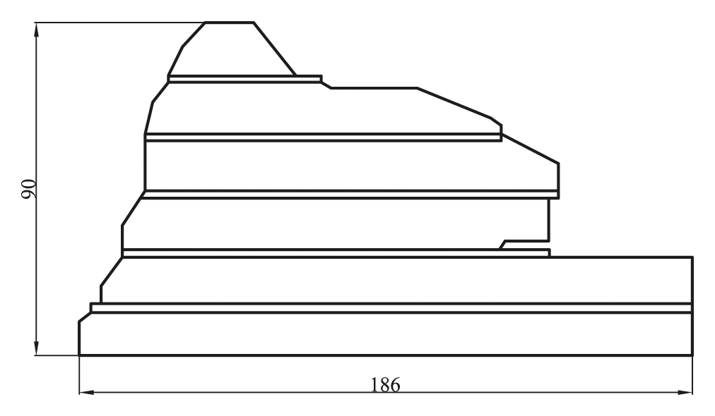
Figure 8: Front-view of the slope on the plane Y = 0 (unit: m)

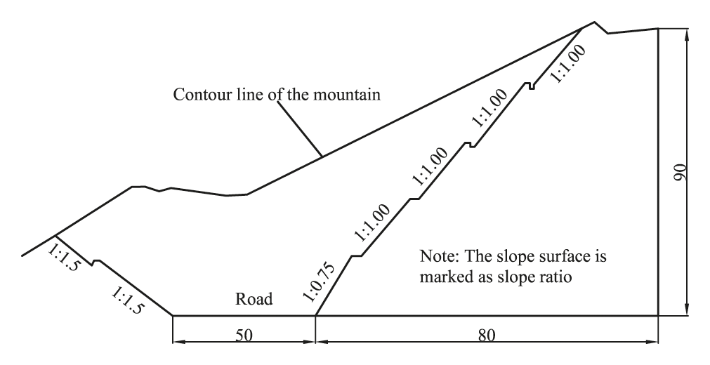
Figure 9: End-view of the slope on the plane X = 0 (unit: m)

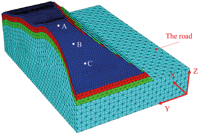
Figure 10: Numerical model of the view

4.1 Criterion I

There is a risk of landslides since the slope along the road is steep. A landslide generally refers to a sudden slide of the sliding body on the sliding surface, accompanied by a sudden increase in displacement from top to bottom. Points on the slope (Fig. 10) are taken as the key points for monitoring displacements. The relationship between the displacement and strength reduction coefficients is depicted in Fig. 11. For point A at the top of the slope, the displacement curve in the Y direction is basically flat, while those in the X and Z directions have obvious mutation points. The displacement in the X direction is less than that in the Z direction when the strength reduction coefficient is smaller than 1.13 but is greater when the strength reduction factor is greater than 1.13. The shapes of the two curves are similar. The displacement grows slowly when the strength reduction coefficient is between 1.00 and 1.10 but increases rapidly when the strength reduction coefficient is between 1.10 and 1.15, indicating that failure begins to take place. When the strength reduction coefficient is between 1.15 and 1.17, the displacement increases exponentially as the strength reduction coefficient increases by 0.01, which indicates that the model is in a failure state. For point B in the middle of the slope, the shape of the curve is basically the same as that of point A. However, the mutation of the curve is more obvious, and the displacements in the Y and Z directions are closer. For point C at the bottom of the slope, the shape of the curve is different from those for the above two points. The curve in Y direction is basically flat. There is no obvious mutation in the displacement curve in the X direction. However, there is evident mutation for the curve in the Z direction. The curve in the Z direction for this point is consistent with those in the X and Z directions for point A, which implies that the shapes of the curves of different points and displacement directions are different. According to this criterion, the FOS of the slope is 1.15.

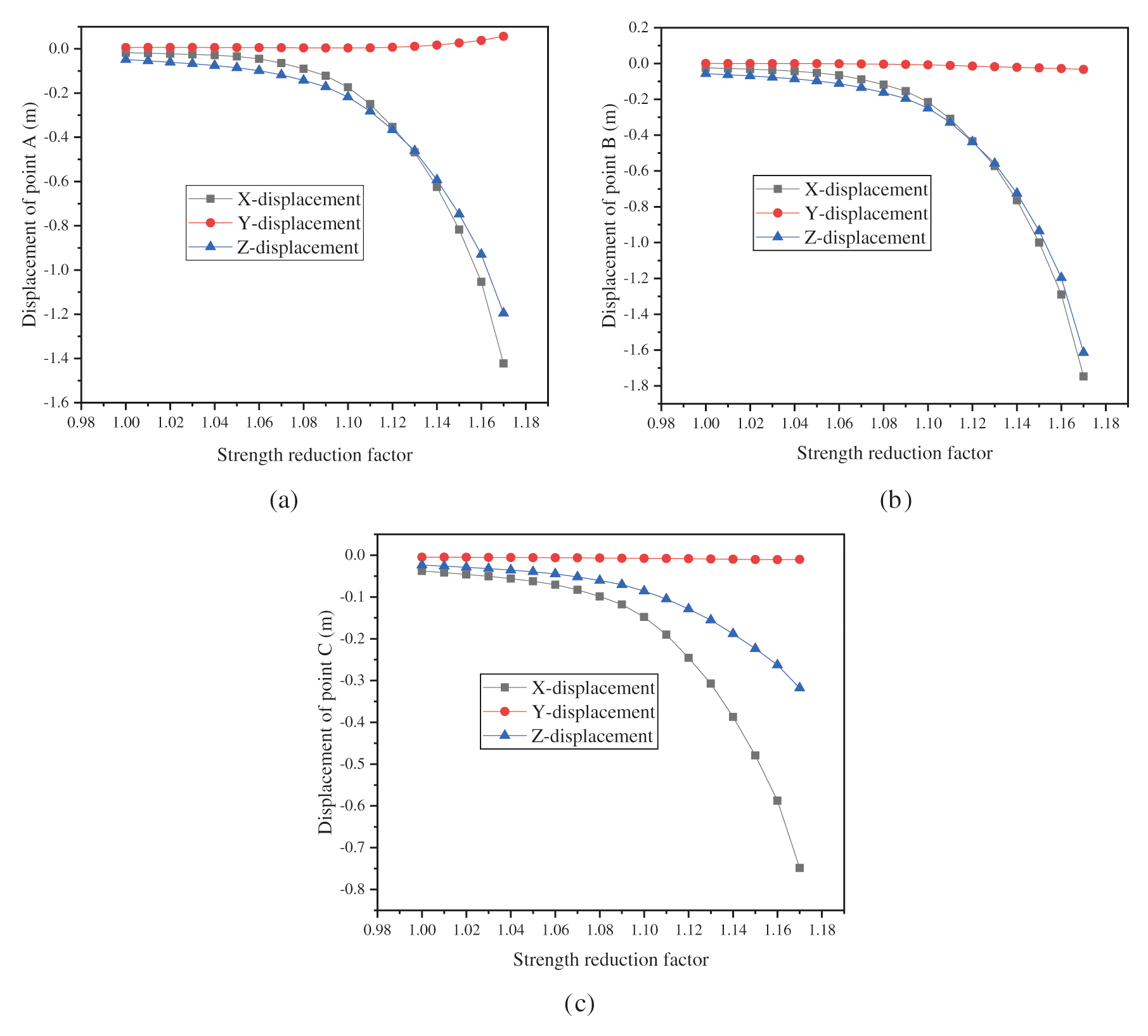
Figure 11: Curves between marked displacements and strength reduction factors

4.2 Criterion II

According to the FISH command, pictures of the zone state of the model under different strength reduction coefficients can be obtained. As shown in Fig. 12, elements with shear failure and tensile cracking failure and without failure are denoted by yellow, red and blue, respectively. When the strength reduction factor is 1.13, a large number of shear yield elements are generated inside the slope. These elements are connected into a block area in the middle but scattered at the model boundary. The yield elements do not form a penetrating slip band, and the slope does not form a landslide condition. The increase in the strength reduction coefficient weakens the strength of the soil and causes the internal elements of the model to bear greater stress and yield. When the strength reduction factor is 1.14, the yield elements in the middle of the model increase, and some are generated on the surface of the slope. The yield elements at the top of the slope are dominated by tensile failure, while those at the bottom are dominated by shear failure. The failure elements are connected to form a penetrating slip band. Forming a landslide condition, the slope tends to slide along the road. As seen from the displacement curves, the displacements in the X direction increase suddenly when the strength reduction coefficient is 1.14. The occurrence of landslides revealed by the displacement curve is consistent with the landslide mechanism revealed by the yield elements in the model. For safety, the FOS of the slope is determined to be 1.13 according to this criterion.

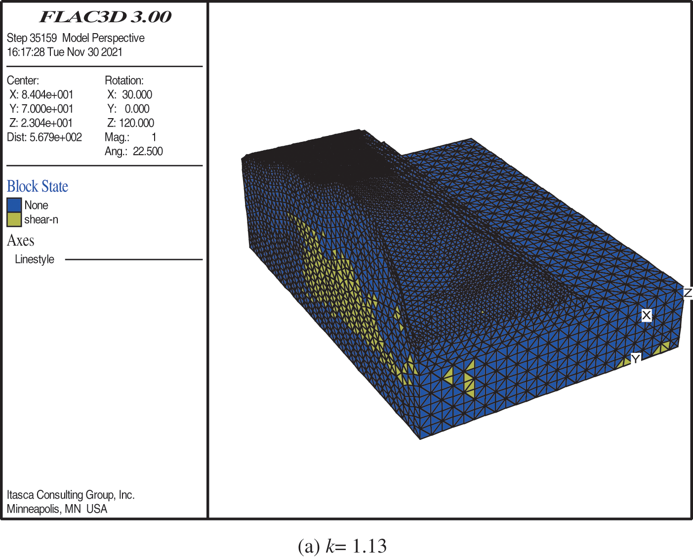
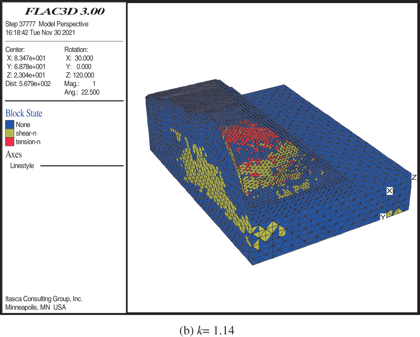
Figure 12: Pictures of the zone state when the strength reduction factor is 1.13 and 1.14 (a) k = 1.13 (b) k = 1.14

4.3 Criterion III

FLAC3D software has a built-in FOS command to calculate the FOS of the slope. The essence of this command is to calculate the FOS under the built-in convergence condition using SRM. However, this command has the disadvantage that the initial upper and lower limits of the strength reduction factor are defined as 0 and 64, respectively, and considerable computation time is required. In this paper, based on the relevant research, a dichotomy strength reduction method is proposed to calculate the FOS. The command stream of the method, written in FISH language, can flexibly apply various constitutive models with high computational efficiency. The calculation process is as follows: first, the lower and upper limits of the strength reduction coefficient are set as 0 and 2. Then, the standard of the calculation convergence that the maximum unbalanced force ratio is 1.0E5 and the limit step number is 10000 is set. After the above, the strength reduction coefficient is divided continuously to be submitted to the model for calculation until the difference between the two strength reduction coefficients is less than 0.01. Finally, the strength reduction coefficient is output as the FOS of the model. According to this criterion, the FOS is given as 1.21.

4.4 Criterion IV

Tu et al. [11] proposed and demonstrated the feasibility and accuracy of criterion IV from the principle of energy conservation. With the help of the finite difference software FLAC3D, the command streams for calculating the elastic and plastic strain energy of the model were programmed. The relationships between the two energy values and the strength reduction coefficients were analyzed based on several two-dimensional slopes and a three-dimensional slope. The FOS of the slope was determined by the mutation of the curves between the energy and strength reduction coefficient. In view of this, a general command stream for calculating the elastic and plastic strain energy of the model is developed in this paper. Both energies can be calculated in all versions of FLAC3D for the convenience of other researchers. The strain energy of the slope under each strength reduction coefficient was calculated, as shown in Fig. 13. In terms of plastic strain energy, there is an obvious mutation in the curve. The energy curve is basically flat without significant change when the strength reduction factor is less than 1.14 and then climbs rapidly when the strength reduction coefficient is between 1.14 and 1.16. When the strength reduction coefficient increases by 0.01, the energy values increase several times, indicating slope failure. In terms of elastic strain energy, the curve has the evident maximum value point. When the strength reduction factor is less than 1.14, the curve grows slowly until reaching its maximum at a strength reduction coefficient of 1.14. When the strength reduction coefficient is between 1.14 and 1.16, the curve shows a downward trend. According to this criterion, the FOS is 1.14.

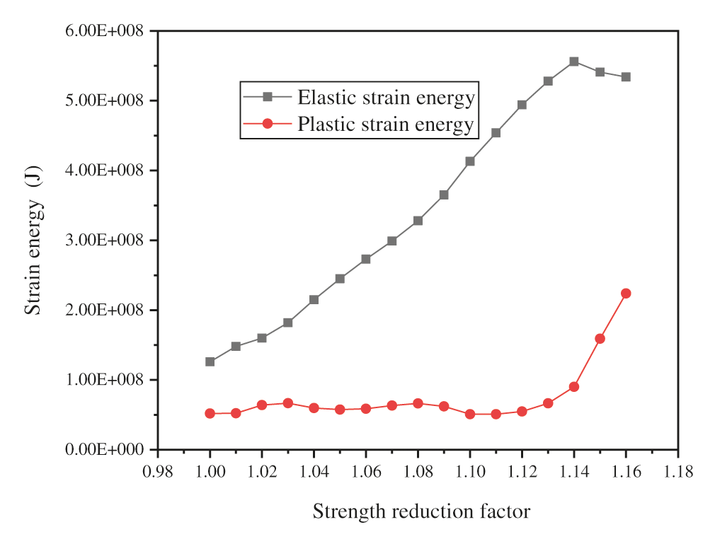
Figure 13: Curves between the slope strain energy and strength reduction factor

4.5 Variational Method

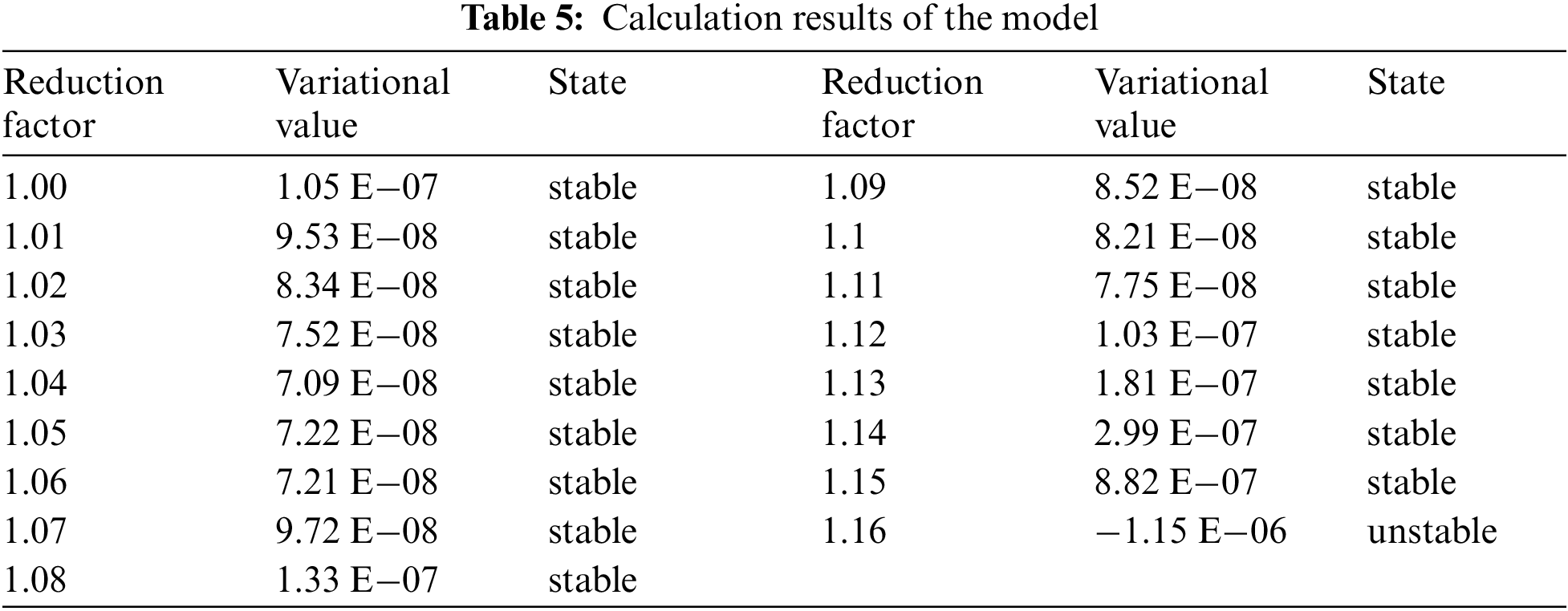
The internal stress and strain of the slope are constantly coupled under the action of force. Most scholars simplify slope stability as the mutation of a single index, namely, the four instability criteria mentioned earlier. These criteria lack mechanical derivation and cannot reflect the internal mechanism of the slope. Considering the above shortcomings, this paper proposes a variational method for determining the slope instability. The results calculated by the variational method are listed in Table 5, which describes the state of the model. The strength reduction coefficient gradually increases from 1.00 to 1.15 with an interval of 0.01. When the strength reduction coefficient is less than or equal to 1.15, the variational value is positive but becomes negative for the first time when the strength reduction coefficient is 1.16. This is consistent with the process of plasticity development and failure of the model, as indicated by other criteria, which suggests that the variational method is accurate. According to this method, the FOS can be confirmed as 1.15, which is close to other criteria.

4.6 Simplified Three-Dimensional Limit Equilibrium Method (STLEM)

To discuss the results of the variational method, LEM is used to calculate the FOS of the slope. The slope is a three-dimensional complex slope with variable geometry and diverse strata. For this type of slope, a typical section is generally selected for calculating the FOS with the slices method. However, the disadvantage of this method is that it weakens the three-dimensional action of the slope and cannot accurately evaluate the safety of the slope. In view of this, a STLEM is proposed to fully consider the three-dimensional characteristics of the slope. According to criterion III, the positions of the sliding surface and sliding body can be obtained when the slope fails. As shown in Fig. 14, the cutting slope produces a landslide along the road, and the sliding surface (red line) consists of silty clay, sandstone 1, and sandstone 2. The slip surface of the three-dimensional curve can be simplified as an oblique plane (blue line). The slide body can be simplified as a pentahedron with a quadrilateral bottom (blue line). The sliding mechanism can be simplified as the plane sliding of the simplified sliding body on the simplified sliding surface. The cohesion is denoted as c0, and the internal friction angle on the sliding surface is denoted as φ0. The bulk density of the sliding body is denoted as γ0. γ0 is the weighted average value based on the thicknesses of the three soil layers. c0 and φ0 are the weighted average values based on the length of the simplified sliding surface across the soil layers. The angle between the simplified sliding surface and the plane x = 0 (the normal vector is n1→) is denoted as ∂0. All these parameters can be calculated by Eq. (8).

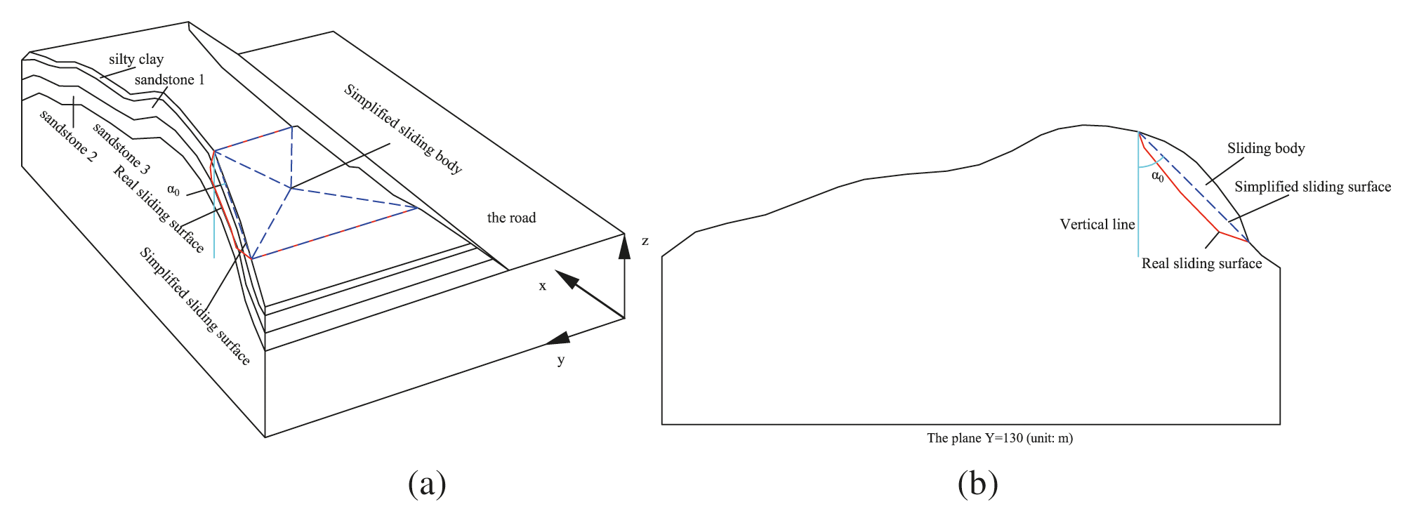
Figure 14: Picture of the sliding surface of the slope

c0=∑i=13cililt φ0=∑i=13φililt γ0=∑i=13γihiht(8)

where ci and φi are the strength parameters for every soil layer. li is the length of the simplified sliding surface across every soil layer. lt is the total length of the simplified sliding surface. γi is the bulk density of every soil layer. hi is the thickness of every soil layer. htis the total thickness of the three soil layers.

The calculation formula of the FOS of the slope is as Eq. (9).

Fs=RF=c0s0+Gsin∂0tanφ0Gcos∂0=c0s0+13γ0s0hsin∂0tanφ013γ0s0hcos∂0=3c0γ0hcos∂0+tan∂0tanφ0(9)

where R and F are the resistance force and slip force of the slope, respectively. s0 is the base area of the pentahedron. It is also the area of the simplified sliding surface. h is the distance from the vertex to the bottom of the pentahedron.

For a particular engineering example, the parameters γ0 can be directly calculated by the strength and thickness of the soil layers. The sliding surface is determined by the contour of the plastic strain increment of the model. According to the contour (criterion III), the lengths of the simplified sliding surface across silty clay, sandstone 1, and sandstone 2 are 6 m, 48 m, and 6 m, respectively. The c0, φ0 can be calculated. The parameters ∂0 and h are computed as follows. Three nonadjacent points on the potential sliding surface are selected, whose coordinates are denoted as p1(x1,y1,z1),p2(x2,y2,z2),p3(x3,y3,z3). The outermost vertex of the sliding body is marked as p4(x4,y4,z4). The relative formulas are given in Eqs. (10)–(14).

n1→=(−1,0,0)(10)

n2→=|ijkx2−x1y2−y1z2−z1x3−x1y3−y1z3−z1|=[(y2−y1)(z3−z1)−(y3−y1)(z2−z1)]i+[(x3−x1)(z2−z1)−(x2−x1)(z3−z1)]j+[(x2−x1)(y3−y1)−(x3−x1)(y2−y1)]k(11)

∂0=cos−1⁡(n1→⋅n2→|n1→||n2→|)(12)

Assuming A=(y2−y1)(z3−z1)−(y3−y1)(z2−z1),B=(x3−x1)(z2−z1)−(x2−x1)(z3−z1),C=(x2−x1)(y3−y1)−(x3−x1)(y2−y1), then the formula for calculating the sliding surface is expressed as:

A(x−x1)+B(y−y1)+C(z−z1)=0(13)

The distance h between the vertex and the sliding surface is:

h=|A(x4−x1)+B(y4−y1)+C(z4−z1)|A2+B2+C2(14)

The corresponding FOS for any four points can be obtained by the relevant calculation formulas. For the engineering example in this paper, four points p1(32.64,132.3,52.9), p2(36.35,132.3,81.84), p3(11.45,95.75,59.9), and p4(19.67,117.3,72.26) are selected. When the known quantities are substituted into the calculation formulas, the following quantities can be obtained: c0=25kPa, φ0=31.90, γ0=20.8kN/m3,∂0=31.70, h=5.4m. The FOS of the slope (marked as Fs) is calculated as Eq. (15).

Fs=3×2520.8×5.4×0.85+tan⁡(31.70)×tan⁡(31.90)=1.16(15)

4.7 Contrasts

The relative error D0 between the variational method and other criteria (or methods) is calculated according to Eq. (7). The calculation results are listed in Table 6. The left column is the FOS under each criterion or method, and the right column is the corresponding relative error.

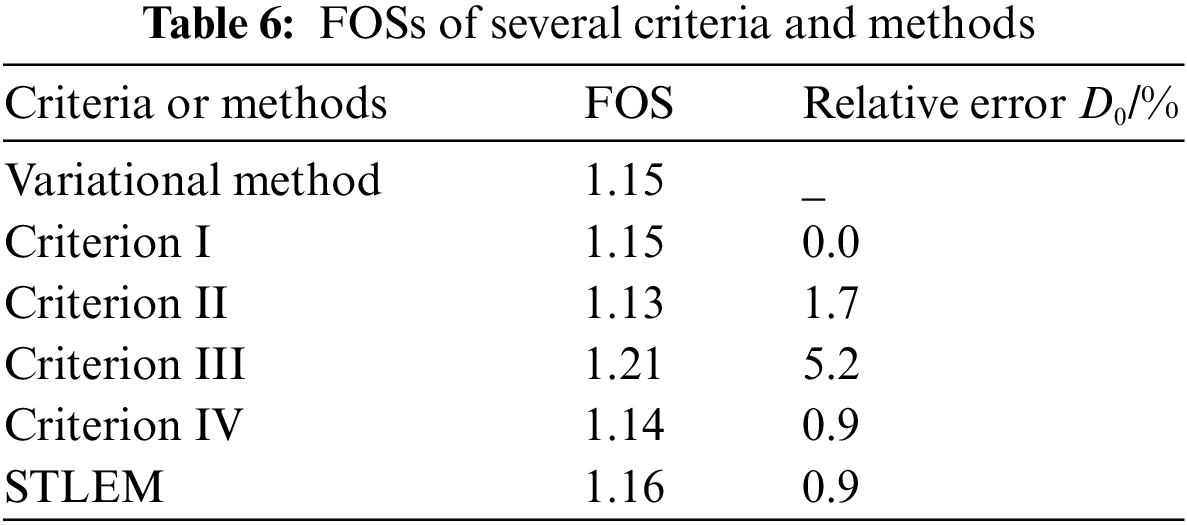
The FOS calculated based on the variational method is consistent with that calculated by criterion I and is slightly greater than those calculated by criterion II and criterion IV, with relative errors of 1.7% and 0.9%, respectively. The value obtained by this method is lower than those obtained by criterion III and the STLEM with relative errors of 5.2% and 0.9% and a maximum error of 5.2%, indicating that the variational method is applicable. The variational method unifies other criteria without identifying the critical areas of the structure and placing monitoring points. The method can comprehensively reflect the coupling effect of stress and strain of the structure, which has more advantages than other criteria. In addition, the method has rigorous mathematical and physical derivation, which provides a mechanical explanation for the instability of the model. Based on the analysis in this paper, the FOS of the cutting slope is 1.15. The slope along the road has a larger gradient, where landslides are the most likely to occur. Special attention should be given to protecting and reinforcing this area.

5  Conclusions

1.    In the field of slope stability analysis, the variational method was proposed against the four widely used instability criteria of SRM. The variational calculation equations of the model were derived, and a variational value calculation program was written in FLAC3D. The FOS obtained by the variational method is consistent with those obtained by other criteria or methods, making the proposed method applicable to inhomogeneous slopes.

2.    The variational method, which consistently reflects the process of slope plasticity and failure, unifies the four criteria, carries out rigorous mathematical and physical derivation, and provides a mechanical basis for determining system stability while overcoming the shortcomings of other criteria.

3.    The general command stream for calculating the elastic and plastic strain energy of the element in FLAC3D software was written to facilitate the application of criterion IV.

Acknowledgement: The authors thank LetPub (https://www.letpub.com) for its linguistic assistance during the preparation of this manuscript.

Funding Statement: The work is supported by the National Natural Science Foundation of China (41807228).

Conflicts of Interest: The authors declare that they have no conflicts of interest to report regarding the present study.

This work is licensed under a Creative Commons Attribution 4.0 International License, which permits unrestricted use, distribution, and reproduction in any medium, provided the original work is properly cited.