| Computer Modeling in Engineering & Sciences |
DOI: 10.32604/cmes.2022.019521
ARTICLE
Enhancing the Effectiveness of Trimethylchlorosilane Purification Process Monitoring with Variational Autoencoder
1Key Laboratory of Advanced Process Control for Light Industry (Ministry of Education), Jiangnan University, Wuxi, 214122, China
2Hangzhou JASU Environmental Monitoring Co., Ltd., Hangzhou, 311999, China
*Corresponding Author: Shunyi Zhao. Email: shunyi.s.y@gmail.com
Received: 27 September 2021; Accepted: 30 December 2021
Abstract: In modern industry, process monitoring plays a significant role in improving the quality of process conduct. With the higher dimensional of the industrial data, the monitoring methods based on the latent variables have been widely applied in order to decrease the wasting of the industrial database. Nevertheless, these latent variables do not usually follow the Gaussian distribution and thus perform unsuitable when applying some statistics indices, especially the
Keywords: Process monitoring; variational autoencoders; partial least square; multivariate control chart
With the increasing demand for product quality and its performance under different industrial environments, the industrial process has become more sophisticated in structure and process flow [1,2]. Therefore, it has been more challenging to ensure their security and reliability while using the model-based modeling approach based on physical and mathematical details [3]. As a substitute for the model-based approach, the data-based modeling approach is regarded as the statistical process control (SPC), which makes outstanding performance on monitoring univariable processes [4,5]. Nevertheless, the behavior of SPC is unsatisfactory while applying to the multivariable processes. For instance, the Type I error rate raises with the number of variables increasing [6]. With the diversification of system parameters, the consequence of this problem has been more and more severe and brings multivariable statistical process control (MSPC) into our sight [7–9].
The most commonly used MSPC charts are Hotelling
where the
Hotelling
where the k and n are the numbers of variables and data and
However, the situation is more complicated when the variables are correlated. The covariance matrix
To determine the Euclidean distance between the original data space and the space of extracted variables and emulate the loss caused by the residual variables [21], we introduce a control chart named SPE to measure the residual loss which has shown as the following Eq. (3).
where
The following Eq. (4) computes the control limit of the SPE chart:
where
Besides the SPE index, we also use the index
where the matrix
where
where
For these two statistics indices,
To solve these sticky problems, we find autoencoder (AE) as an effective solution. As an essential sub-field in data analysis [23], AE acts as a bridge that can connect big machinery data and intelligent monitoring [24]. Its unsupervised learning property signifies it does not require label data [25] which is hard to obtain in modern industry processes [26]. AE is composed of the input layers called the encoder, the hidden layer, and the output layers called the decoder [27]. The encoder is an efficient dimensional reduction algorithm for high-dimensional data [28]. It decreases the dimension not in the way that reduces some dimensions by mathematical calculation. Instead, it mapped the data to a low dimension state by encoding and is able to decode these reduced data to the original dimension through the decoder [29]. As a result, AE has a significant function that its output is equivalent to its input [30]. The operating principle of its encoder can be regarded as a combination of several neural networks which can resolve the nonlinear problem because their mapping structure and activation function is used to add nonlinear factors to argue the expression ability of these networks.
Another problem is that the input data of
In this paper, we proposed a method that combined the PLS and VAE. The combination algorithm will apply to the trimethylchlorosilane purification process to verify its superiority over other traditional algorithms. The characteristic of the PLS algorithm represents that the monitoring statistics are determined by both the independent variable and dependent variable. It means that its latent variable contains the information of both dependent and independent variables, which is different from the latent variable extracted by the VAE algorithm that is only correlated with the independent variable. We use the PLS to extract the more informative latent variable and bring it as the input dataset of VAE. And the VAE algorithm maps the input dataset to latent distribution that follows the Gaussian distribution. In this way, we obtain the latent variable that is more informative and follows the hypothesis of the monitoring indices. The flow chart of our proposed algorithm is shown in Fig. 1.
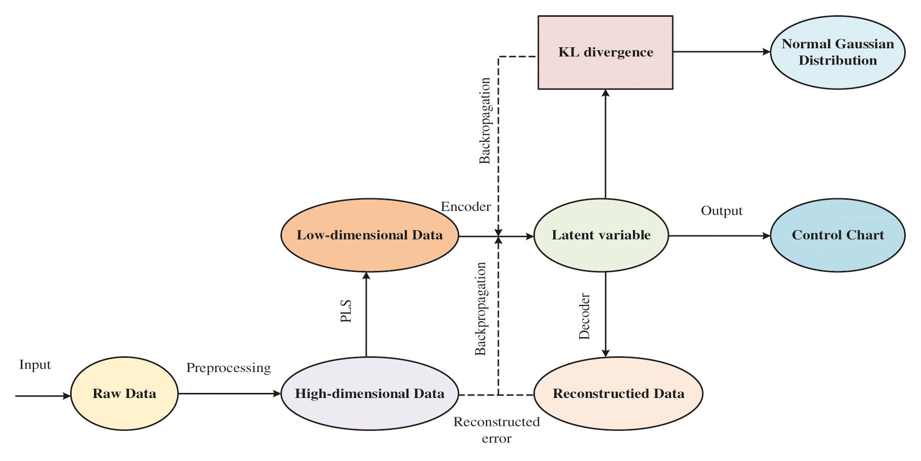
Figure 1: The flow chart of proposed algorithm
The contributions of this paper are displayed as follows:
(1) We integrate the PLS method with the VAE method. The main idea of this method is to use the PLS method to transfer the data from the original space to a low-dimensional space that can save the correlation information between the independent and dependent variables. And applying the VAE method, which can address the difficulty that the extracted latent variables do not follow the Gaussian distribution and nonlinear process. To integrate the PLS and VAE method, we first use the PLS method to decrease the data dimensions, then apply these processed data to VAE to extract their latent variables and calculate the statistic index
(2) We make a comparison in both simulation and real industrial process with some other methods, which are also on the basis of the latent variables. To verify the superiority of the proposed method, we use the false alarm rate, which statistics indices are more significant than the calculated control limit, to measure the accuracy of these methods, and their result is displayed in the form of the picture.
The rest of this paper is organized as follows. In Section 2, we will introduce the principle and structure of the PLS and VAE model. Then we will represent the PLS algorithm in Algorithm 1, the VAE algorithm in Algorithm 2 and demonstrate how to integrate these two algorithms with
2.1 Partial Least Squares (PLS)
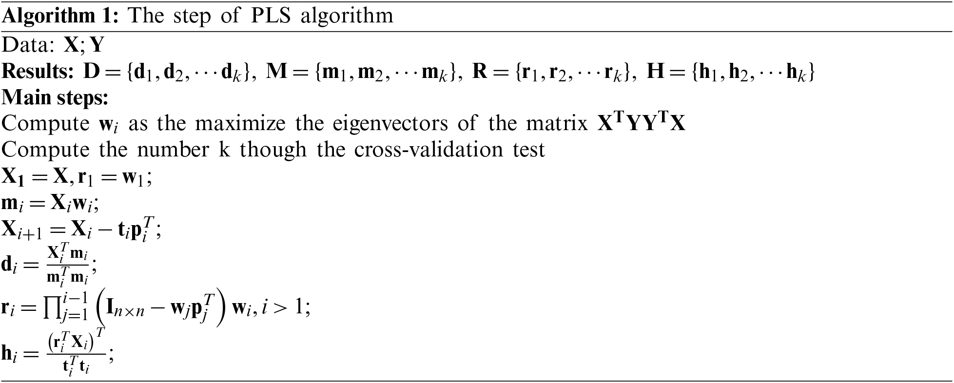
The partial least squares (PLS) algorithm has some properties similar to principal component analysis (PCA), which is used to decrease the dimensions of the original data. The PLS algorithm can be used to make regression modeling analysis, reduce the data dimension, and correlation analysis which means that PLS integrates the using fields and advantages of the multiple linear regression algorithms, principal component analysis algorithm, canonical correlation analysis algorithm.
The PLS is widely used when the input vector
The independent variable
where n is the number of components extracted from variables and its value is determined by a kind of statistical techniques such as cross-validation.
2.2 Variational AutoEncoder (VAE)
Variational AutoEncoder (VAE) has been widely used in data analysis which is essential in data-based modeling. The VAE can be used as a generative model whose purpose is to produce a database
The generative procedure can be described in two steps. First, a distribution
The distribution
where
Now, we should find the variational lower bound of
And that means the features of the original database that follow Gaussian distribution can be extracted by doing these, which is beneficial in applying the common statistics index like
In our study, a simple distribution is often used to approximate a complex distribution. At this time, we need a quantity to measure how much information the approximate distribution we choose has lost compared to the original distribution, which is how the KL divergence works. By constantly changing the parameters of the approximate distribution, we can get different values of KL divergence. In a specific range of variation, when the KL divergence reaches the minimum value, the corresponding parameter is the optimal parameter we want. When the
As is shown in Fig. 2, the encoder
We denote the weight matrix as
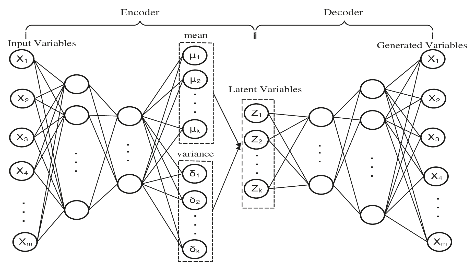
Figure 2: The architecture of variational AutoEncoder
And the nodes in the
where the
During the training process, the model needs to back-propagate the error through all the layers in order to decrease the error. However, the layer that sampling
where
After gaining the Gaussian feature
where
The decoder is the opposite of the encoder both the structure and the transferred information. The input of the decoder is the latent variables
Because the generated data set is printed by the decoder
where the
These two parameters can be used to build the SPE control chart, the equation of SPE and the control limit are represented as the following Eqs. (22) and (23).
where
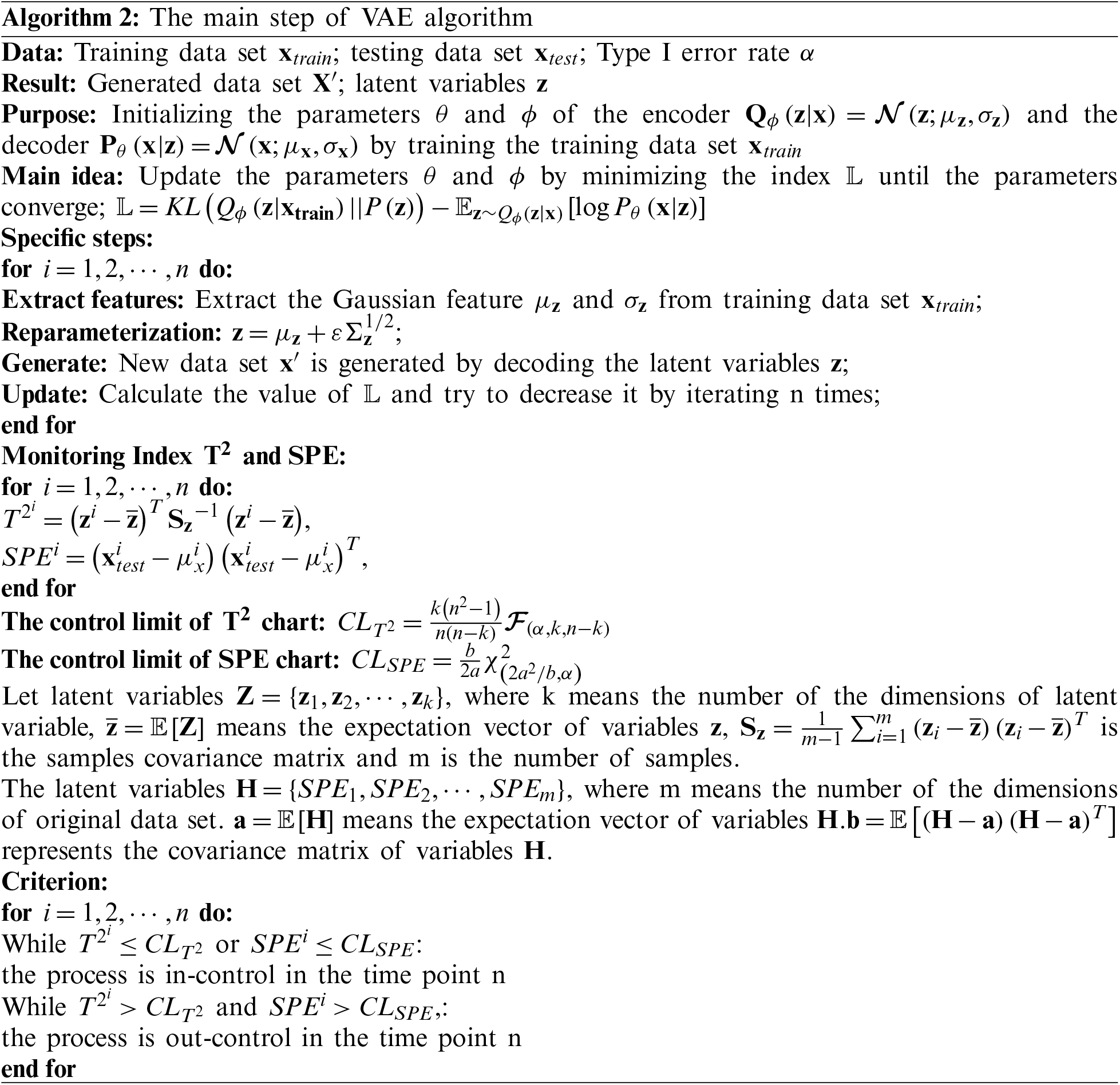
Different from the traditional VAE-based algorithm and VAE based algorithm that merely reduce the dimensions of all input variables, the PLS-VAE based algorithm utilizes the characteristic of the PLS model to produce latent variables which contain the information between independent and dependent variables. Then we input these latent variables into the VAE model, acquire some new latent variables by the encoder, and use them to calculate the
The main step of the calculation of
This simulation is built to examine the superior of the PLS-VAE algorithm by comparing it to other methods based on latent variables. In this case, we choose the VAE, PLS, AE methods and test their performance under different conditions. We use several kinds of data distributions as inputs included the normal and non-normal database. The non-normal database included the Chi2 distribution representing the skewed situation, the t-distribution that denotes the symmetric process and the gamma distributions which stands for the kurtosis industrial process. We use the ratio of the actual Type I error rate and the expected Type I error rate to be a criterion to assess the performance of these monitoring methods. In these four distributions, we generated 1000 data which contains 900 in-control data and 100 out-control data, and every data is composed of 100 and 300 variables, respectively. To be closer to the actual industrial process, we generate a column that is a linear combination of all variables. This column is used to simulate the output variable which is affected by input variables.
We build a VAE model which is consists of seven fully connected hidden layers. The architecture of the VAE model included three hidden layers both in the encoder and decoder and one hidden layer in the middle, which is built for the latent variables.
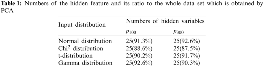
The complete architecture is shown in Fig. 2. We use the tanh function as the activation function. To make a comparison, we build four models which are PLS based model, AE based model, VAE based model and PLS-VAE based model. To be equal, we use the same hyperparameters of the VAE model including the number of layers, the quantity of nodes and the activation function. We choose the PCA method to ensure the amount of the extracted variables in these four models can bear the weight of the vast majority of dimensions of the original data set. And the reason we choose the PCA is that the algorithm can easily obtain the ratio of each extracted component in the whole variance. As is shown in Table 1, the first 25 principal components account for nearly 90 percent of the entire data in normal distribution, which means that we can use 25 principal components to substitute all the data. Table 1 shows the ratio of the first 25 components in each distribution.
As for the hyperparameters in VAE, we use 0.001 as the learning rate, which is commonly used in the deep learning field. The loss function is optimized by Adam optimizer with 0.001 learning rate. The mean squared error is assigned as the standard to weigh up the loss function to get minimized by training.
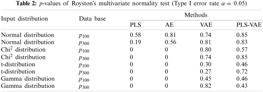
The VAE model has a function that can transform the non-normal distribution to normal distribution, which can improve the performance of the
where
The specific production process is as follows:
1. We generate 900 samples of 100 process variables
2. We introduce anomalies at the 901st sample point by making
3. The first 900 samples will be combined with these 100 samples as a complete dataset.
We input the original database to PLS, AE, VAE, PLS-VAE methods and test the extracted feature to verify whether it has this function. The result is shown in Table 2. According to this table, only when the input data follows the normal distribution, the extracted features also follow the normal distribution in all methods. On the contrary, the latent features extracted in the VAE architecture follow the normal distribution.
We compare the performance of these four different methods by the ratio of the actual Type I error rate and the expected Type I error rate. We use different values of Type I error rate from the range 0.02 to 0.2. The control chart result is shown in Fig. 3. In these pictures, the line generated by these ratio points is treated as better when they get closer to the 45 degree line because this line means the actual model obtain the same value as the expected one. These pictures confirm that the control charts which have VAE structure get better performance than other control charts because the expected rate it generates is more similar to their corresponding actual rate, which means its curved line is closer to the 45 degree line. Some lines are overlapped because some different methods get the same value. In the non-normal case, we find that the
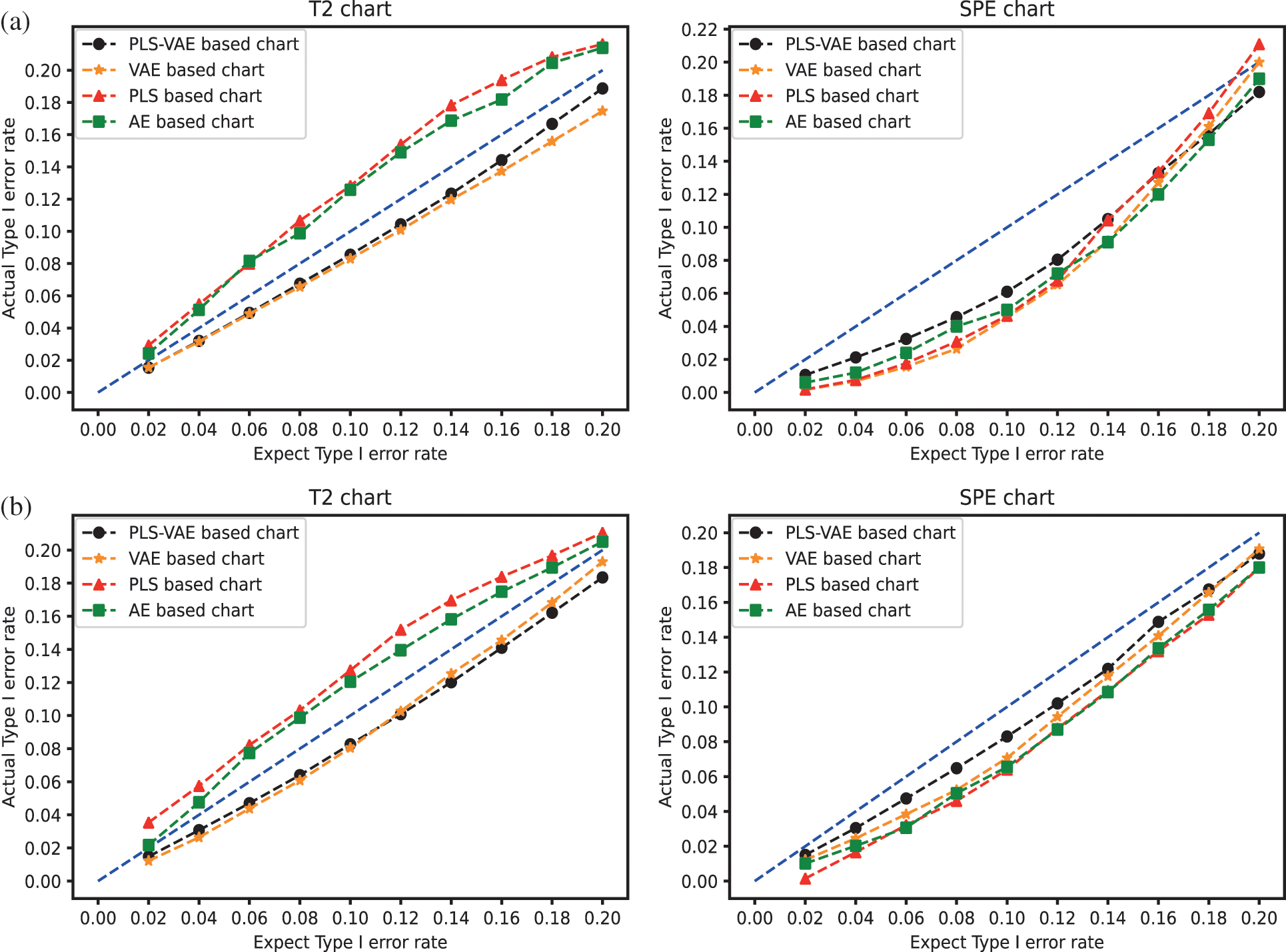
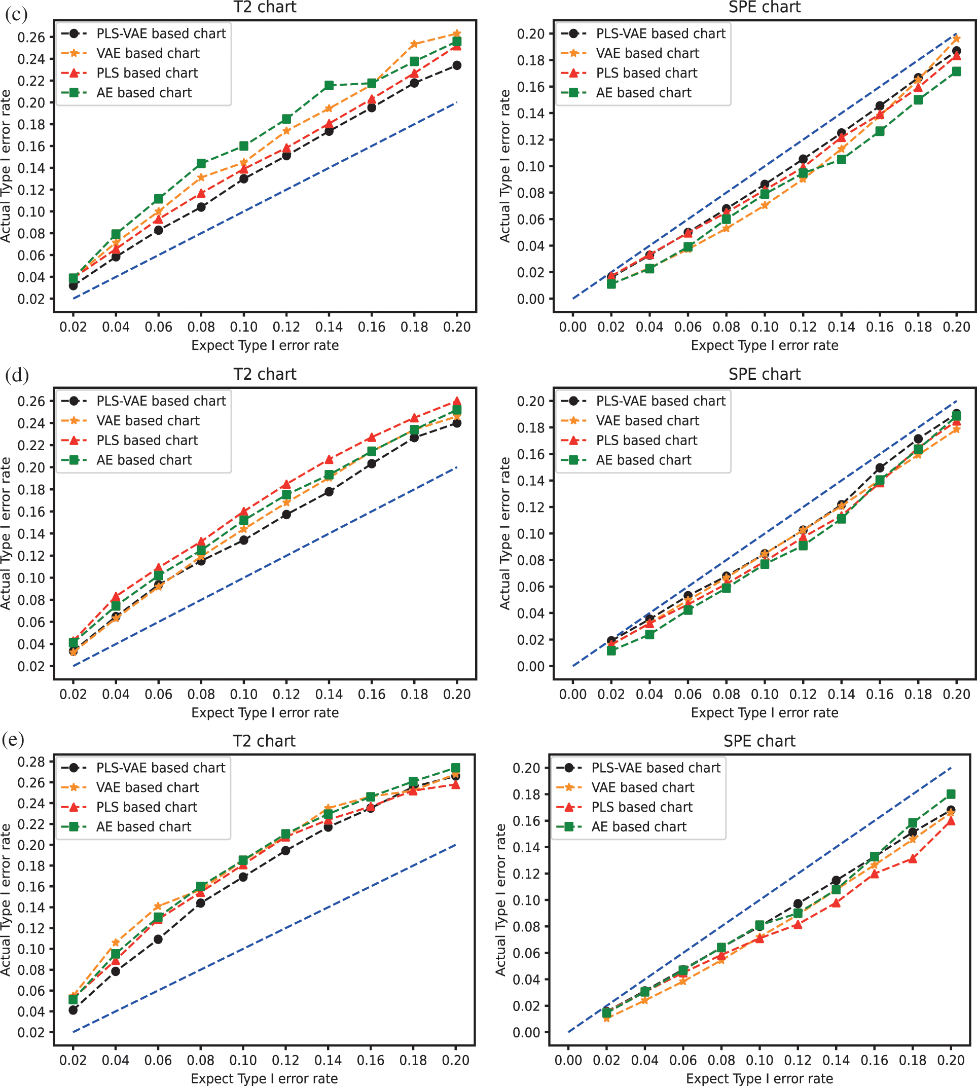
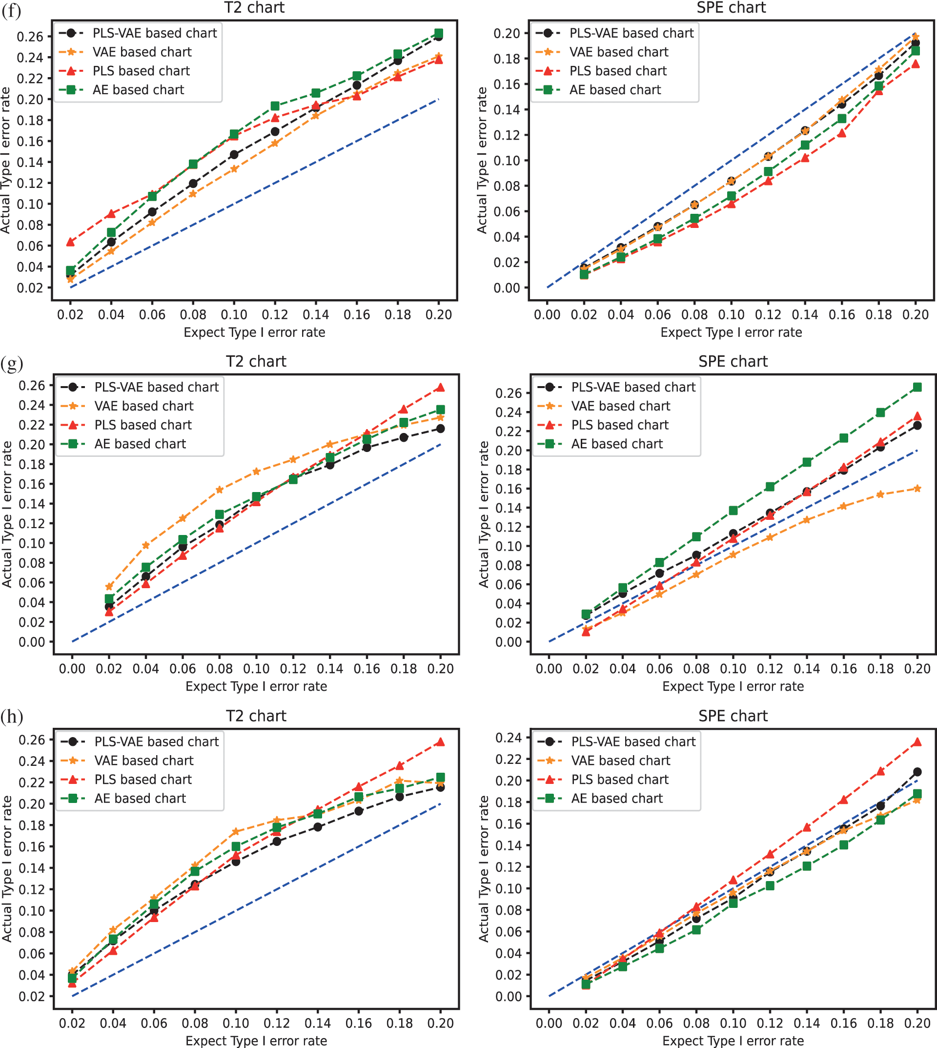
Figure 3: The
4.1 Description of Trimethylchlorosilane Purification Process
The separation and purification process and system of Trimethylchlorosilane mixed monomer is composed of several processes included distillation separation, extraction, cyclic reaction. At present, the organic silicon monomer separation process which is commonly used is the direct sequence. In this sequence, the crude monomer sends through the high-removal tower and low-removal tower firstly, then gets into the binary tower to detach monomethyltrichlorosilane and dimethyldichlorosilane. The product collected on the top of the low-removal tower has been extracted from the low boiler component in the light detachment tower and the trimethylchlorosilane component in the trimethylchlorosilane tower. The high boiler component of the material in the tower kettle of the De-high tower is separated through the high boiler tower. In this process, the azeotrope component collected from the azeotrope tower is not easy to solve. The material in both the top of the high boiler tower and the tower kettle of trimethylchlorosilane tower need to get back in the former system and separate monomethyltrichlorosilane and dimethyldichlorosilane product from it. Because of the high standard to the purity of product, any tiny fluctuations of the process may make the products disqualified.
Our study focuses on the process links which monitoring object is the secondary cooling material liquid phase outlet. This link plays an integral part in the Trimethylchlorosilane purification process because its production determines the degree of the purity of the final production. The process which is directly relevant to this link is demonstrated in Fig. 4. The facility of this process link is composed of a reboiler which is used to supply the energy to the distillation tower, a distillation tower which is used to distil some kinds of products that we need from the top of the tower, a condenser which is using for condensing the input material and a reflux accumulator which refluxes to the distillation tower by a bump.
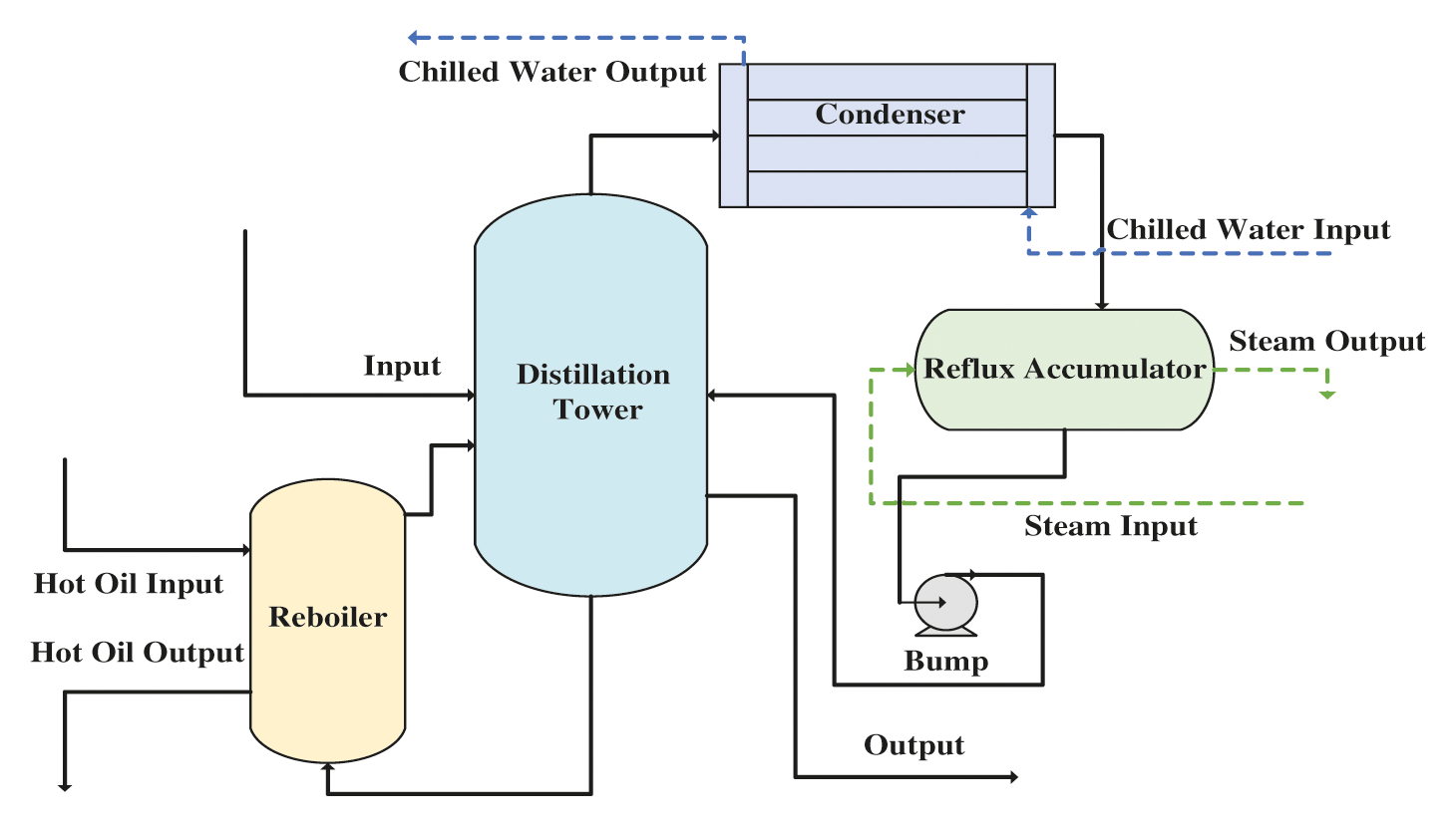
Figure 4: The process flow of the Trimethylchlorosilane purification
4.2 Analysis of the Industrial Process
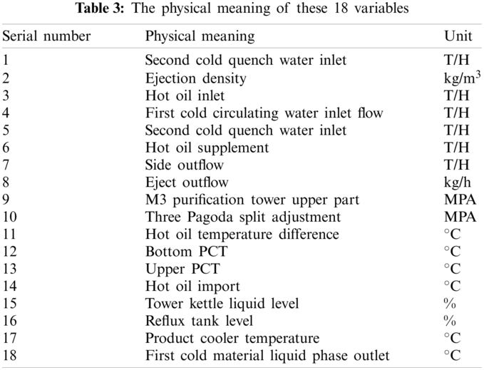
In this case, we obtain 1000 observed data composed of 18 variables from the Trimethylchlorosilane purification process. The physical meaning of these 18 variables is shown in Table 3. The first seventeen variables are treated as the independent variables, while the last one is the dependent variable of the Trimethylchlorosilane purification process. In this process, the input of the proposed method is these 1000 observed data composed of 18 variables, and the output is the control charts shown in Fig. 5.
To determine the ultimate model establish methods, we compare the monitoring control chart of PLS-, AE-, VAE- and PLS-VAE-based charts and the Type I error rate α = 0.05. The multi-variable control chart based on these methods is shown in Figs. 5a–5d, respectively. In this study, we choose the
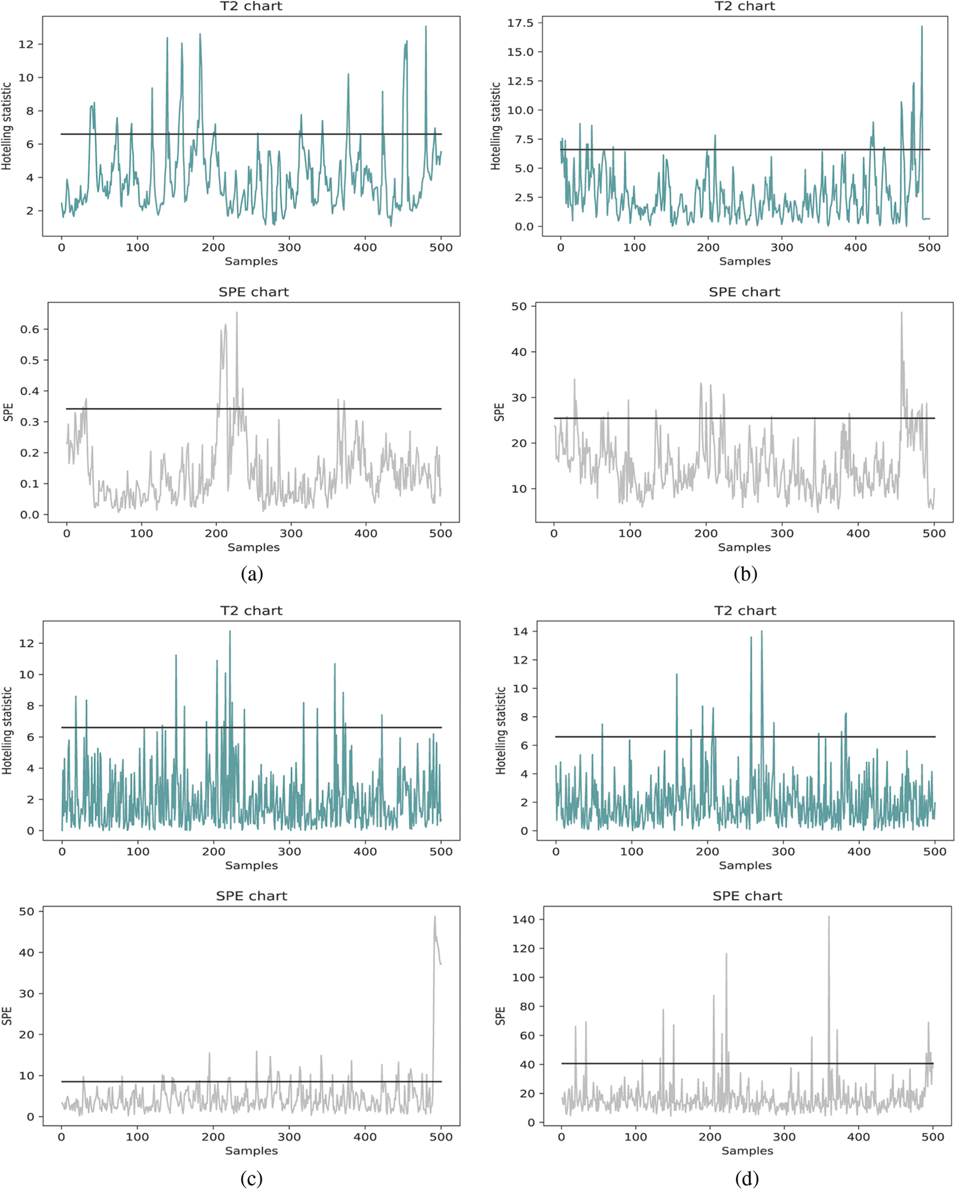
Figure 5: The control charts of different monitoring methods: (a) PLS based chart (b) AE based chart (c) VAE based chart (d) PLS-VAE based chart
To test the accuracy of the model we established, we input the test data set into the model training by the training data set and record the process quality indexes. Then, we input the test data set into the model training by itself and record the quality indexes. The comparative standard of the T2 and SPE control chart is the actual false alarm rates and the expected false rate of the PLS-, AE-, VAE- and PLS-VAE-based charts. The actual rate is calculated from the former model, while the expected rate is obtained from the latter one. The ratio between these two rates is shown in Fig. 6a, which is represented the performance of each method. The 45 degree line means the actual rate is equal to the expected rate, which is the best circumstance, and the line which is closest to the 45 degree line performs better than others, especially when the value of the range is less than 0.15. And the value we usually choose is 0.05, thus we can determine that the PLS-VAE is better. Fig. 6b shows the ratio between the actual false rate and expected false rate of the SPE statistics. The criterion standard is also the distance to 45 degree line. And the resulting figure shows the proposed method is closer to the standard line, which means it performs better than other methods.
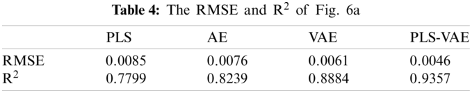
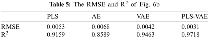
The model fit in Fig. 6 does not look particularly clear. In order to make it more clarity, the RMSE and R2 of Fig. 6 are shown in Tables 4 and 5. In this tables, we can find that the RMSE and R2 of PLS-VAE perform better than others.
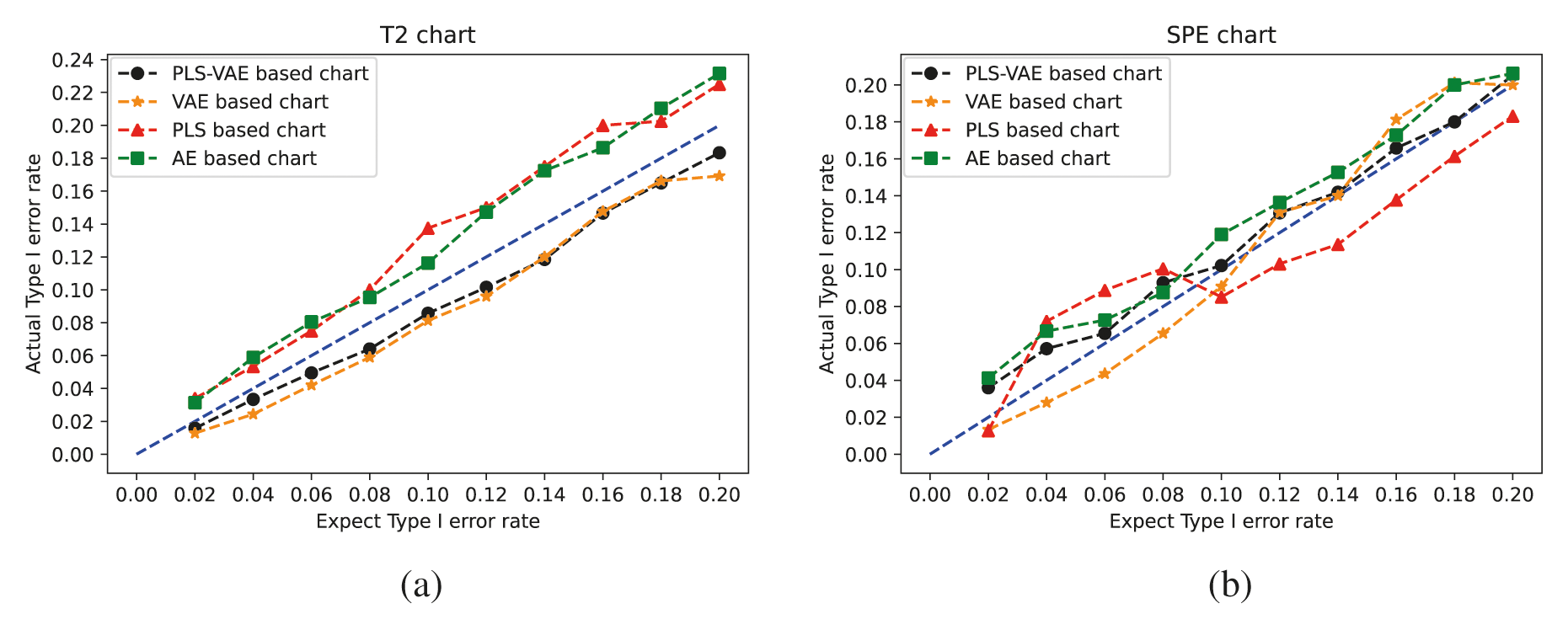
Figure 6: Comparison between these methods by the ratio of the actual Type I error rate and the expected Type I error rate: (a)
In this paper, we propose applying the PLS-VAE based control chart to monitor the multi-variables process when the input data is not following the Gaussian distribution and has a relationship between the dependent variables and independent variables. Compared to the AE model, VAE can extract the latent variable which is forced to follow the Gaussian distribution by decreasing the KL divergence between the latent distribution and the normal distribution
Our next workshop will focus on the integration between the fields of deep learning, such as VAE and some other traditional control methods. The target fields may be the multiple model process and some other process that is suitable for data-based control methods. We will also try to bring its generative ability into process monitoring and fault detection especially when the number of data is obtained scarcely and costly.
Funding Statement: The authors received no specific funding for this study.
Conflicts of Interest: The authors declare that they have no conflicts of interest to report regarding the present study.
1. Ge, Z., Chen, J. (2015). Plant-wide industrial process monitoring: A distributed modeling framework. IEEE Transactions on Industrial Informatics, 12(1), 310–321. DOI 10.1109/TII.2015.2509247. [Google Scholar] [CrossRef]
2. Zhou, K., Liu, T., Zhou, L. (2015). Industry 4.0: Towards future industrial opportunities and challenges. 2015 12th International Conference on Fuzzy Systems and Knowledge Discovery (FSKD), pp. 2147–2152. Zhangjiajie, China. [Google Scholar]
3. Tidriri, K., Chatti, N., Verron, S. (2016). Bridging data-driven and model-based approaches for process fault diagnosis and health monitoring: A review of researches and future challenges. Annual Reviews in Control, 42(8), 63–81. DOI 10.1016/j.arcontrol.2016.09.008. [Google Scholar] [CrossRef]
4. Ge, Z., Liu, Y. (2018). Analytic hierarchy process based fuzzy decision fusion system for model prioritization and process monitoring application. IEEE Transactions on Industrial Informatics, 15(1), 357–365. DOI 10.1109/TII.2018.2836153. [Google Scholar] [CrossRef]
5. Jiang, Q., Yan, X., Huang, B. (2019). Review and perspectives of data-driven distributed monitoring for industrial plant-wide processes. Industrial & Engineering Chemistry Research, 58(29), 12899–12912. DOI 10.1021/acs.iecr.9b02391. [Google Scholar] [CrossRef]
6. Gupta, M., Kaplan, H. C. (2017). Using statistical process control to drive improvement in neonatal care: A practical introduction to control charts. Clinics in Perinatology, 44(3), 627–644. DOI 10.1016/j.clp.2017.05.011. [Google Scholar] [CrossRef]
7. Ji, H., He, X., Shang, J. (2017). Incipient fault detection with smoothing techniques in statistical process monitoring. Control Engineering Practice, 62(2), 11–21. DOI 10.1016/j.conengprac.2017.03.001. [Google Scholar] [CrossRef]
8. Wang, Y., Si, Y., Huang, B. (2018). Survey on the theoretical research and engineering applications of multivariate statistics process monitoring algorithms: 2008–2017. The Canadian Journal of Chemical Engineering, 96(10), 2073–2085. DOI 10.1002/cjce.23249. [Google Scholar] [CrossRef]
9. He, Q. P., Wang, J. (2018). Statistical process monitoring as a big data analytic tool for smart manufacturing. Journal of Process Control, 67, 35–43. DOI 10.1016/j.jprocont.2017.06.012. [Google Scholar] [CrossRef]
10. Ahsan, M., Mashuri, M., Lee, M. H. (2020). Robust adaptive multivariate Hotelling's T2 control chart based on kernel density estimation for intrusion detection system. Expert Systems with Applications, 145(15), 113105. DOI 10.1016/j.eswa.2019.113105. [Google Scholar] [CrossRef]
11. Draisma, J., Horobeţ, E., Ottaviani, G. (2016). The Euclidean distance degree of an algebraic variety. Foundations of Computational Mathematics, 16(1), 99–149. DOI 10.1007/s10208-014-9240-x. [Google Scholar] [CrossRef]
12. Mostajeran, A., Iranpanah, N., Noorossana, R. (2018). An explanatory study on the non-parametric multivariate T2 control chart. Journal of Modern Applied Statistical Methods, 17(1), 12. DOI 10.22237/jmasm/1529418622. [Google Scholar] [CrossRef]
13. Dong, Y., Qin, S. J. (2018). A novel dynamic algorithm for dynamic data modeling and process monitoring. Journal of Process Control, 67(1), 1–11. DOI 10.1016/j.jprocont.2017.05.002. [Google Scholar] [CrossRef]
14. Wen, L., Li, X., Gao, L. (2017). A new convolutional neural network-based data-driven fault diagnosis method. IEEE Transactions on Industrial Electronics, 65(7), 5990–5998. DOI 10.1109/TIE.2017.2774777. [Google Scholar] [CrossRef]
15. Ge, Z. Q. (2017). Review on data-driven modeling and monitoring for plant-wide industrial processes. Chemometrics and Intelligent Laboratory Systems, 171(2), 16–25. DOI 10.1016/j.chemolab.2017.09.021. [Google Scholar] [CrossRef]
16. Dijkstra, T. K., Henseler, J. (2015). Consistent partial least squares path modeling. MIS Quarterly, 39(2), 297–316. DOI 10.25300/MISQ/2015/39.2.02. [Google Scholar] [CrossRef]
17. Tong, C., Lan, T., Yu, H. (2019). Distributed partial least squares based residual generation for statistical process monitoring. Journal of Process Control, 75(2017), 77–85. DOI 10.1016/j.jprocont.2019.01.005. [Google Scholar] [CrossRef]
18. Harrou, F., Nounou, M. N., Nounou, H. N. (2015). PLS-based EWM fault detection strategy for process monitoring. Journal of Loss Prevention in the Process Industries, 36(1), 108–119. DOI 10.1016/j.jlp.2015.05.017. [Google Scholar] [CrossRef]
19. Muradore, R., Fiorini, P. (2012). A PLS-based statistical approach for fault detection and isolation of robotic manipulators. IEEE Transactions on Industrial Electronics, 59(8), 3167–3175. DOI 10.1109/TIE.2011.2167110. [Google Scholar] [CrossRef]
20. Mehmood, T. (2016). Hotelling T2 based variable selection in partial least squares regression. Chemometrics and Intelligent Laboratory Systems, 154(3), 23–28. DOI 10.1016/j.chemolab.2016.03.001. [Google Scholar] [CrossRef]
21. Tôrres, A. R., Junior, S. G. (2015). Multivariate control charts for monitoring captopril stability. Microchemical Journal, 118, 259–265. DOI 10.1016/j.microc.2014.07.017. [Google Scholar] [CrossRef]
22. Chen, J., Liu, K. C. (2002). On-line batch process monitoring using dynamic PCA and dynamic PLS models. Chemical Engineering Science, 57(1), 63–75. DOI 10.1016/S0009-2509(01)00366-9. [Google Scholar] [CrossRef]
23. Yin, S., Li, X., Gao, H. (2015). Data-based techniques focused on modern industry: An overview. IEEE Transactions on Industrial Electronics, 62(1), 657–667. DOI 10.1109/TIE.2014.2308133. [Google Scholar] [CrossRef]
24. Sisinni, E., Saifullah, A., Han, S. (2018). Industrial Internet of Things: Challenges, opportunities, and directions. IEEE Transactions on Industrial Informatics, 14(11), 4724–4734. DOI 10.1109/TII.2018.2852491. [Google Scholar] [CrossRef]
25. Lund, D., MacGillivray, C., Turner, V. (2014). Worldwide and regional Internet of Things (IOT) 2014–2020 forecast: A virtuous circle of proven value and demand. Technical Report Series, 1(19. International Data Corporation (IDC). [Google Scholar]
26. Zhao, R., Yan, R., Chen, Z., Mao, K., Wang, P. et al. (2019). Deep learning and its applications to machine health monitoring. Mechanical Systems and Signal Processing, 115(1), 213–237. DOI 10.1016/j.ymssp.2018.05.050. [Google Scholar] [CrossRef]
27. Suh, S., Chae, D. H., Kang, H. G. (2016). Echo-state conditional variational autoencoder for anomaly detection. International Joint Conference on Neural Networks (IJCNN), pp. 1015–1022. Vancouver, BC, Canada. [Google Scholar]
28. Lee, S., Kwak, M., Tsui, K. L. (2019). Process monitoring using variational autoencoder for high-dimensional nonlinear processes. Engineering Applications of Artificial Intelligence, 83(7), 13–27. DOI 10.1016/j.engappai.2019.04.013. [Google Scholar] [CrossRef]
29. Meng, Q., Catchpoole, D., Skillicom, D. (2017). Relational autoencoder for feature extraction. International Joint Conference on Neural Networks (IJCNN), pp. 364–371. Anchorage, AK, USA. [Google Scholar]
30. Liou, C. Y., Cheng, W. C., Liou, J. W. (2014). Autoencoder for words. Neurocomputing, 139(5210), 84–96. DOI 10.1016/j.neucom.2013.09.055. [Google Scholar] [CrossRef]
31. Xu, W., Tan, Y. (2019). Semisupervised text classification by variational autoencoder. IEEE Transactions on Neural Networks and Learning Systems, 31(1), 295–308. DOI 10.1109/TNNLS.2019.2900734. [Google Scholar] [CrossRef]
32. Zhang, Z., Jiang, T., Zhan, C. (2019). Gaussian feature learning based on variational autoencoder for improving nonlinear process monitoring. Journal of Process Control, 75(2), 136–155. DOI 10.1016/j.jprocont.2019.01.008. [Google Scholar] [CrossRef]
33. Xie, R., Hao, K., Chen, L., Huang, B. (2020). Supervised variational autoencoders for soft sensor modeling with missing data. IEEE Transactions on Industrial Informatics, 16(4), 2820–2828. DOI 10.1109/TII.2019.2951622. [Google Scholar] [CrossRef]
34. Hemmer, M., Klausen, A., Khang, H. V. (2020). Health indicator for low-speed axial bearings using variational autoencoders. IEEE Access, 8, 35842–35852. DOI 10.1109/ACCESS.2020.2974942. [Google Scholar] [CrossRef]
35. Yan, X., She, D., Xu, Y. (2021). Deep regularized variational autoencoder for intelligent fault diagnosis of rotor-bearing system within entire life-cycle process. Knowledge-Based Systems, 226(6), 107142. DOI 10.1016/j.knosys.2021.107142. [Google Scholar] [CrossRef]
36. Zhang, K., Tang, B., Qin, Y. (2019). Fault diagnosis of planetary gearbox using a novel semi-supervised method of multiple association layers networks. Mechanical Systems and Signal Processing, 131(5786), 243–260. DOI 10.1016/j.ymssp.2019.05.049. [Google Scholar] [CrossRef]
37. Cheng, F., He, Q. P., Zhao, J. (2019). A novel process monitoring approach based on variational recurrent autoencoder. Computers & Chemical Engineering, 129(17), 106515. DOI 10.1016/j.compchemeng.2019.106515. [Google Scholar] [CrossRef]
38. Zhu, J., Shi, H., Song, B. (2020). Information concentrated variational autoencoder for quality-related nonlinear process monitoring. Journal of Process Control, 94, 12–25. DOI 10.1016/j.jprocont.2020.08.002. [Google Scholar] [CrossRef]
 | This work is licensed under a Creative Commons Attribution 4.0 International License, which permits unrestricted use, distribution, and reproduction in any medium, provided the original work is properly cited. |