| Computer Modeling in Engineering & Sciences |
DOI: 10.32604/cmes.2022.020412
ARTICLE
Accelerated Iterative Learning Control for Linear Discrete Systems with Parametric Perturbation and Measurement Noise
1School of Energy and Architecture, Xi'an Aeronautical University, Xi'an, 710077, China
2School of Automation, Northwestern Polytechnical University, Xi'an, 170072, China
*Corresponding Author: Saleem Riaz. Email: saleemriaznwpu@mail.nwpu.edu.cn
Received: 22 November 2021; Accepted: 31 December 2021
Abstract: An iterative learning control algorithm based on error backward association and control parameter correction has been proposed for a class of linear discrete time-invariant systems with repeated operation characteristics, parameter disturbance, and measurement noise taking PD type example. Firstly, the concrete form of the accelerated learning law is presented, based on the detailed description of how the control factor is obtained in the algorithm. Secondly, with the help of the vector method, the convergence of the algorithm for the strict mathematical proof, combined with the theory of spectral radius, sufficient conditions for the convergence of the algorithm is presented for parameter determination and no noise, parameter uncertainty but excluding measurement noise, parameters uncertainty and with measurement noise, and the measurement noise of four types of scenarios respectively. Finally, the theoretical results show that the convergence rate mainly depends on the size of the controlled object, the learning parameters of the control law, the correction coefficient, the association factor and the learning interval. Simulation results show that the proposed algorithm has a faster convergence rate than the traditional PD algorithm under the same conditions.
Keywords: Iterative learning control; monotone convergence; convergence rate; gain adjustment
The system has gradually become one of the most highly debated research topics in the field of control in recent years [1]. The system is a type of important hybrid system that consists of a set of differential equations, finite differences, and switching rules that change based on actual environmental factors, enabling the whole system to switch between different subsystems to adapt to the demands of different conditions on the system and improve system performance [2]. Therefore, the system is widely used in practical engineering systems, such as traffic control systems [3], power systems, circuit systems [4], network control systems [5], etc. At present, many research results related to the system are focused on the system's stability [6], but the research results on the output tracking control of the system are very limited [7]. The reason is that the tracking control of the system is much more difficult to achieve than the stabilization and stability problem.
Iterative learning control [8] has a simple structure, does not require specific model parameters, and can make the behavior of the executed object meet the expected requirements only after enough iterations in a limited interval. This learning algorithm has been widely employed in the control of rigid robot arms [9], batch processing in the process industry [10], aerodynamic systems [11], traffic control systems [12], electrical and power systems, and other areas due to the characteristics as mentioned earlier [13]. However, most scholars focus on non-system control problems, and research on system iterative learning control problems is limited [14].
In industrial applications, the controlled system parameters are usually time-varying, so the classical PID and combined PID-like control schemes are particularly inflexible when dealing with the system with uncertain factors [15–17]. In addition, the analysis and design process of some existing modern control schemes [18] is complex and difficult. The designed control algorithm and structure should be simple enough and easy to implement to solve these problems. The control scheme should contain the characteristics of nonlinearity, robustness, flexibility and learning ability. With the rapid development of intelligent control technology to solve the uncertainty and complexity of the controlled object, some neural network models and neural network training schemes have been applied to the design of system controllers [19]. For example, as a feedforward controller, Plett [20] discussed how neural networks learn to imitate the inverse of the controlled object. However, the neural network has the disadvantages of slow learning speed and weak generalization ability, and there is no systematic method to determine its topology. Suppose there is not a timely manner sable control and compensation. In that case, the system noise and random interference will appear in the input end of the controller, which will greatly reduce the stability of the adaptive process and seriously affect the control accuracy. Adaptive filtering has been widely developed [21,22], and neural network is the most commonly used in all kinds of nonlinear filtering. However, it is highly nonlinear in terms of parameters [23–25].
Above mentioned scholars are studying the model uncertainty in different fields such as model prediction, system identification [26], fault detection [27], motor control [28], and nonlinear control [29]. Still, there is no specific control algorithm for satisfactory fast error convergence and specific to consider the system coupling, uncertainty, time-varying characteristics, measurement noise and other factors. Adaptive control strategy is proposed in these literature [30–32] which can compensate at some extent. An adaptive control is mainly used to deal with complex nonlinear systems with unknown parameters. Based on Lyapunove stability theory, parameter novelty law is designed to achieve system stabilization and progressive tracking of target trajectory [33,34]. Both some special nonlinear systems linearized to parameters [35,36] and nonlinear systems with general structures [37] have achieved remarkable development. For systems that cannot be modeled or contain un-modeled states, literature [38,39] proposed the model-free adaptive control theory. However, these adaptive control methods cannot solve the problem of complete tracking over a finite time interval [40].
This paper emphases on a class of discrete time-invariant arbitrary systems that perform repeating tracking tasks on an expected trajectory in a finite time interval based on the above analysis. A PD type is taken as an example, under the condition that the switching sequence is randomly determined, and the iteration is unchanged, by applying characteristics of iterative learning control, provide a discrete iterative learning control algorithm with error backward association to correct control quantity of the next iteration. Combined with the theory of hypervector and spectral radius, the algorithm's convergence is discussed, and sufficient conditions for the algorithm's convergence are given theoretically.
The article can be divided in different sections in order to demonstrate the contribution briefly. The Main contribution and results are comprised in the following sections. Problem formulation is briefly described in Section 2. The convergence analysis, theory of hypervector, spectral radius, and the sufficient conditions for the error convergence are elaborated in Section 3. Then the following Section 4 has showed the numerical example for the validity of the proposed algorithm. Finally, the results summarization of this paper is described in Section 5.
Consider the following class of linear discrete time-invariant single input and single output systems with repetitive parameter perturbation and measurement noise over a finite period:
where
Here,
In the iterative learning process of the system (1), the expected trajectory is set as
Assumption 1. In each system iteration, the initial state is equal to the ideal initial state, i.e.,
Assumption 2. Expects trajectory
Assumption 3. For any given desired trajectory
Basing on system (1), define
For ease of description, write the above expression in the form of a hypervector, and introduce a hypervector:
The above equation can be description as
where
*represents an uncertain value by the dynamics and uncertain parameters of the system (1).
System (1), under the condition that assumption 1–3 satisfied, considers a control rule of error backward association and subsequent control quantity correction:
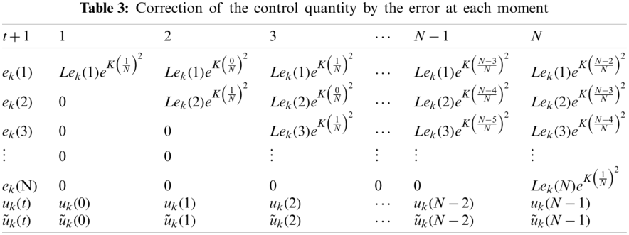
The correction of the error before time t to the control quantity at the current time
The learning control rule of PD type iterative as
where
The correction of control quantity (5a) is explained in detail below, as shown in Fig. 1. In the learning process of the
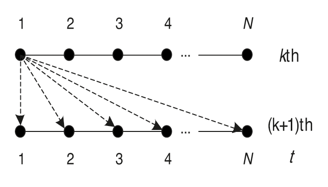
Figure 1:
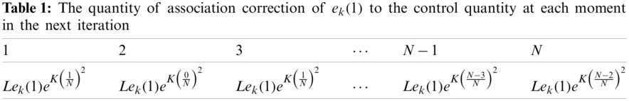
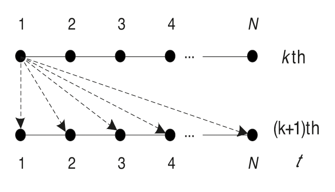
Figure 2:
According to this method, up to the point, its error is
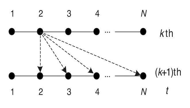
Figure 3:
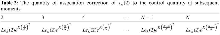
According to the above analysis, the correction quantity of each error to the control quantity of following moments can be plotted. The correction
which is consistent with Eq. (5a).
Lemma 1 Let
Proof With triangle inequality of norm,
Lemma 2 Let
Proof Necessity. Let A to be a convergency matrix, because of properties spectral radius,
Sufficiency. Since
3.1 Case of a Determined Model Without Measurement Noise
Theorem 1 Consider a linear discrete time-invariant system (1) with single-input and single-output. If assumption 1–3 is satisfied, the system model is determined, and no measurement noise is obtained;
Then the output trajectory uniformly converges to the expected trajectory, that is, when
Proof According to the iterative learning control algorithm (5), in the
If we introduce the following hypervector
Then we have
where,
Since the model is determined and has no measurement noise, i.e.,
According to Lemma 2, the necessary and sufficient condition of
It is easy to know that the necessary and sufficient condition for the convergence of the system is
The theorem is proved. I would like to explain this further about the convergence which is basically shows the output within the finite time interval
3.2 Case of the Undetermined Model without Measurement Noise
Theorem 2 Consider a linear discrete time-invariant system (1) with single-input and single-output. If assumption 1–3 is satisfied, the system model is uncertain but there is no measurement noise, i.e.,
Then the output trajectory uniformly converges to the expected trajectory, that is, when
Proof The control rule Eq. (8) is still available. Since the system model is determined and there is no measurement noise, i.e.,
According to Lemma 2, the necessary and sufficient condition of
The necessary and sufficient condition for the convergence of the system is
The theorem is proved.
3.3 Case of the Determined Model with Measurement Noise
If the model is determined and has measurement noise, i.e.,
Let
When
When
When
For the repetitive perturbation,
When
For non-repetitive perturbations, assume that the two-interval perturbations are bounded; there is a positive real number
Theorem 3 Consider a linear discrete time-invariant system (1) with single input and a single output. If assumption 1–3 is satisfied, and there is non-repetitive measurement noise
Then the system's output converges to a certain neighbourhood of the expected trajectory, that is, when
Proof Eq. (10) is still valid. For the non-repeatable perturbations, there is a positive real number
Take the norm of both sides of Eq. (10)
If
According to above analysis, the sufficient condition for system convergence is
and the error will converge to a boundary, which is
The Theorem 3 is proved.
3.4 Case of Undetermined Model with Measurement Noise
If the system model is not determined and contains measurement noise, that is,
Define
When
When
When
For the repetitive perturbation
For non-repetitive perturbations, assume that the two interval perturbations are bounded, that is, there is a positive real number
Theorem 4 Consider a linear discrete time-invariant system (1) with single-input and single-output. If assumption 1–3 is satisfied, and there is non-repetitive measurement noise
Then the output of the system converges to A certain neighborhood of the expected trajectory, that is, when
Proof Eq. (13) still holds, and take the norm to both sides of the equation
If
According to above analysis, the sufficient condition for system convergence is
and the error will converge to a boundary, which is
Depiction on people's association thinking, this paper proposes a new type of association iterative learning control algorithm, which, with the help of kernel function (a monotonically decreasing function), uses the information of the present time to make prediction and correction of the future control input in the current iterative process. The information of the current time corrects the subsequent unlearned time, the closer the current time, the greater the influence, the smaller the opposite. Obviously, the kernel function makes the association iterative learning algorithm more reasonable. In the process of theoretical proof of convergence analysis, the kernel function is eliminated, so it is not reflected in the convergence condition. It is proved that the association algorithm and the traditional iterative learning control have the same convergence conditions, but the simulation result of the fifth part of the paper shows that the algorithm does have much better convergence speed than the traditional iterative learning algorithm.
In order to verify the validity of the associative correction learning rule proposed in this paper, a class of linear discrete time-invariant single-input single-output systems with repetitive parameter perturbation and measurement noise in a finite time period is considered
where:
4.1 Case of Determined Model without Measurement Noise
If the system model is determined and there is no measurement noise, i.e.,
Let the iterative proportional gain
satisfies the convergence condition.
If
The expected trajectory is
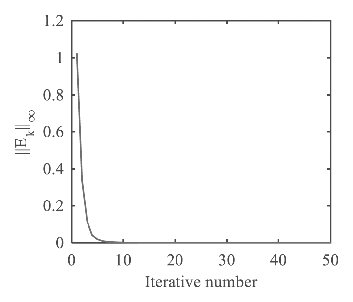
Figure 4: The variation trend of the norm of error of accelerated ILC algorithm with the increasing number of iterations
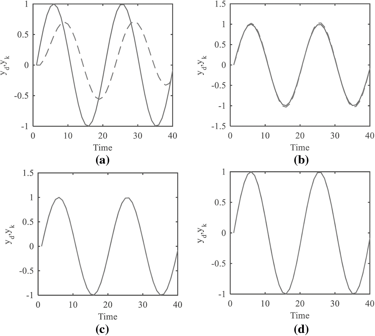
Figure 5: Output trajectory and expected trajectory (a) After the first iteration (b) After the fifth iteration (c) After the seventh iteration (d) After the 11th iteration
When the traditional PD-type learning rule is applied, let the iterative proportional gain
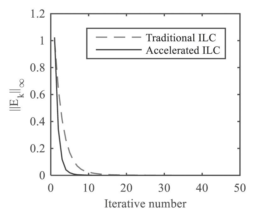
Figure 6: Error comparison between the traditional algorithm and the accelerated algorithm
4.2 Case of the Undetermined Model with Measurement Noise
If the system model is not determined and contains measurement noise, that is,
The matrix pairs
Assume
where
meet the convergence condition, while
Expected trajectory is
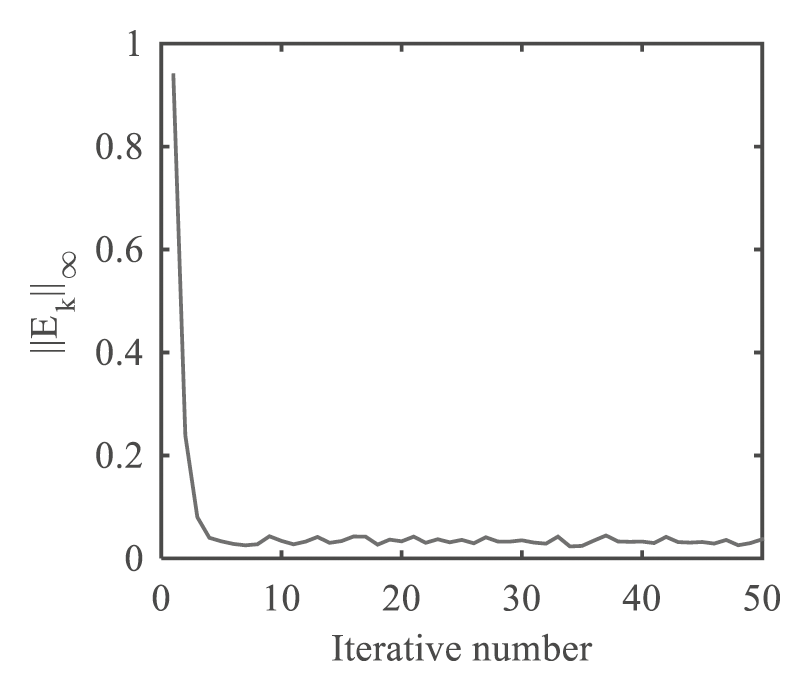
Figure 7: The variation trend of the norm of error of accelerated ILC algorithm with increasing number of iterations
In order to observe of the convergence process of the output trajectory, Fig. 8 shows the comparison plots of the system output and the expected trajectory after the first, fourth, seventh and 11th iterations.
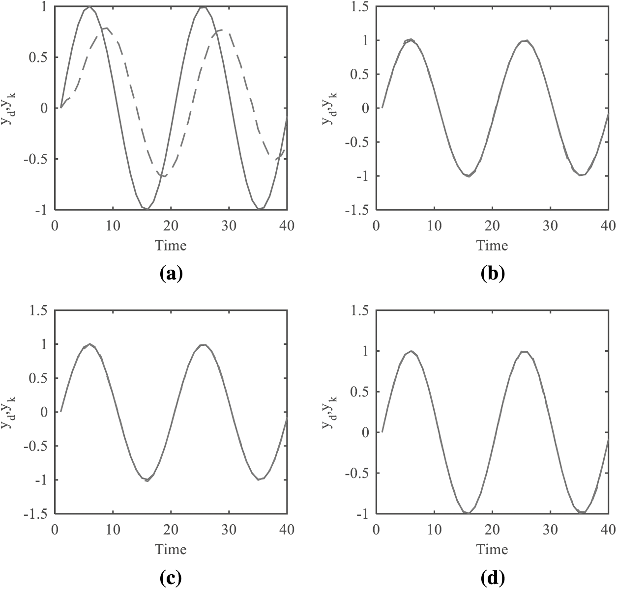
Figure 8: Comparison of system output and desired trajectory (a) After the first iteration (b) After the fourth iteration (c) after the 7th iteration (d) after the 11th iteration
If we take
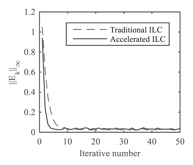
Figure 9: Comparison of error convergence rate between traditional PD-type learning rule and accelerated learning rule
It can be seen from the Fig. 9 that the system tracking error does not converge to 0, but to a boundary. Theorem 4,
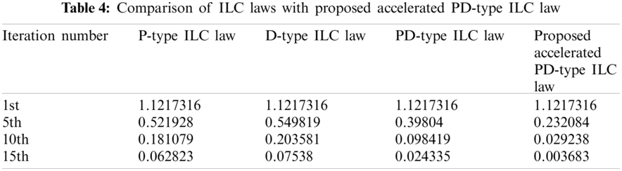
Table 4 shows that the tracking error of P, D, PD and accelerated proposed PD type ILC laws in the first iteration is 1.1217316. After 15th iterations, the error of the P-type law is 0.062823, D type algorithm is 0.07538, and the error of algorithm PD law is 0.024335. Where the error of the proposed accelerated PD law is 0.003683, from the column of Table 4 to the data, the tracking error of all ILC law is reduced consecutively with the increase of iteration number. However, from the horizontal data in Table 4, the tracking error of the proposed accelerated PD law is the smallest as compared to other ILC laws (P, D, PD) under the same iteration number. Therefore, it can be easily observed from Table 4 that the convergence speed of the proposed accelerated PD law in this paper is significantly higher than that of other traditional laws.
The auto-associative ILC proposed in this paper is based on the traditional ILC, namely, using the current information to estimate the future input. Compared to traditional ILC, the new algorithm is characterized as follows: in each trial, the unlearned time is pre-corrected with the current time information. The algorithm can reduce the number of iterations and accelerate the learning convergence speed. The algorithm proposed in this paper differs from the traditional discrete closed-loop algorithm and the higher-order algorithm as follows:
(1) Although the algorithm proposed in this paper is similar in form to the traditional closed-loop iterative learning algorithm, the principle is completely different from that of the traditional discrete closed-loop PD-type algorithm (feedback algorithm). The traditional discrete closed-loop ILC algorithm is to correct the control input of the current time directly with the error of the previous time in the same trial. The algorithm proposed in this paper uses the error of the current time to pre-estimate the amount of control after which it does not occur at all times, and plays the role of pre-correction.
(2) Although the associative iterative learning algorithm proposed in this paper is similar in form to the traditional higher-order discrete learning algorithm, the learning process is completely different from the traditional higher-order iterative learning algorithm. The traditional high-order ILC is the algebraic overlay of the control information of the previous two or more trials at the corresponding time. The new iterative learning algorithm proposed in this paper is to pre-correct the subsequent unoccurred time with the error value of the current time in the same trial.
The problem of discrete linear time-invariant systems with parameter perturbation and measurement noise is investigated in this paper. It proposes sufficient conditions for convergence of a PD-type accelerated iterative learning algorithm with association correction under the circumstances of parameter determined without measurement noise, parameter undetermined without noise, parameter determined with measurement noise. Parameter undermined with measurement noise, respectively. Under the same simulation conditions, the convergence radius of the proposed algorithm is smaller than that of the traditional PD-type ILC algorithm. The convergence is theoretically proven with the help of hyper vector and spectral radius theory. Numerical simulation shows the effectiveness of the proposed algorithm. The results show that the algorithm can fully track the expected trajectory within finite intervals when uncertain system parameters. In the case of measurement noise existing, the system's output will converge to a neighborhood of the expected trajectory using the algorithm proposed in this paper. In future studies, we will consider the stability and convergence of nonlinear discrete systems with parameter perturbations and measurement noises and the convergence of arbitrary bounded changes of initial conditions.
Acknowledgement: I want to declare on behalf of my co-authors that the work described is original research that has not been published previously and is not under consideration for publication elsewhere, in whole or in part. I confirmed that no conflict of interest exists in submitting this manuscript and is approved by all authors for publication in your journal.
Funding Statement: The authors received no specific funding for this study.
Conflicts of Interest: The authors declare that they have no conflicts of interest to report regarding the present study.
1. Lin, H., Antsaklis, P. J. (2009). Stability and stabilizability of switched linear systems: A survey of recent results. IEEE Transactions on Automatic Control, 54(2), 308–322. DOI 10.1109/TAC.2008.2012009. [Google Scholar] [CrossRef]
2. Liberzon, D., Morse, A. S. (1999). Basic problems in stability and design of switched systems. IEEE Control Systems Magazine, 19(5), 59–70. DOI 10.1109/37.793443. [Google Scholar] [CrossRef]
3. Balluchi, A., di Benedetto, M. D., Pinello, C., Rossi, C., Sangiovanni-Vincentelli, A. N. D. A. (1999). Hybrid control in automotive applications: The cut-off control. Automatica, 35(3), 519–535. DOI 10.1016/S0005-1098(98)00181-2. [Google Scholar] [CrossRef]
4. Wang, X., Zhao, J. (2013). Partial stability and adaptive control of switched nonlinear systems. Circuits, Systems, and Signal Processing, 32(4), 1963–1975. DOI 10.1007/s00034-012-9544-5. [Google Scholar] [CrossRef]
5. Yu, J., Wang, L., Yu, M. (2011). Switched system approach to stabilization of networked control systems. International Journal of Robust and Nonlinear Control, 21(17), 1925–1946. DOI 10.1002/rnc.1669. [Google Scholar] [CrossRef]
6. Cheng, D., Guo, L., Lin, Y., Wang, Y. (2005). Stabilization of switched linear systems. IEEE Transactions on Automatic Control, 50(5), 661–666. DOI 10.1109/TAC.2005.846594. [Google Scholar] [CrossRef]
7. Riaz, S., Lin, H., Mahsud, M., Afzal, D., Alsinai, A., et al. (2021). An improved fast error convergence topology for PDα-type fractional-order ILC. Journal of Interdisciplinary Mathematics, 24(7), 2005–2019. [Google Scholar]
8. Arimoto, S., Kawamura, S., Miyazaki, F. (1984). Bettering operation of robots by learning. Journal of Robotic Systems, 1(2), 123–140. DOI 10.1002/(ISSN)1097-4563. [Google Scholar] [CrossRef]
9. Liu, J., Wang, Y., Tong, H. T., Han, R. P. (2012). Iterative learning control based on radial basis function network for exoskeleton arm. 2nd International Conference on Advances in Materials and Manufacturing Processes (ICAMMP 2011), vol. 415–417, pp. 116–122. DOI 10.4028/www.scientific.net/AMR.415-417.116. [Google Scholar] [CrossRef]
10. Sanzida, N., Nagy, Z. K. (2013). Iterative learning control for the systematic design of supersaturation controlled batch cooling crystallisation processes. Computers & Chemical Engineering, 59, 111–121. DOI 10.1016/j.compchemeng.2013.05.027. [Google Scholar] [CrossRef]
11. Tan, K. K., Lim, S. Y., Lee, T. H., Dou, H. (2000). High-precision control of linear actuators incorporating acceleration sensing. Robotics and Computer-Integrated Manufacturing, 16(5), 295–305. DOI 10.1016/S0736-5845(00)00009-0. [Google Scholar] [CrossRef]
12. Hou, Z., Yan, J., Xu, J. X., Li, Z. (2011). Modified iterative-learning-control-based ramp metering strategies for freeway traffic control with iteration-dependent factors. IEEE Transactions on Intelligent Transportation Systems, 13(2), 606–618. DOI 10.1109/TITS.2011.2174229. [Google Scholar] [CrossRef]
13. Feng, X., Zhang, Y., Kang, L., Wang, L., Duan, C. et al. (2021). Integrated energy storage system based on triboelectric nanogenerator in electronic devices. Frontiers of Chemical Science and Engineering, 15(2), 238–250. DOI 10.1007/s11705-020-1956-3. [Google Scholar] [CrossRef]
14. Ruan, X., Zhao, J. (2013). Convergence monotonicity and speed comparison of iterative learning control algorithms for nonlinear systems. IMA Journal of Mathematical Control and Information, 30(4), 473–486. DOI 10.1093/imamci/dns034. [Google Scholar] [CrossRef]
15. Srivastava, S., Pandit, V. S. (2016). A PI/PID controller for time delay systems with desired closed loop time response and guaranteed gain and phase margins. Journal of Process Control, 37, 70–77. DOI 10.1016/j.jprocont.2015.11.001. [Google Scholar] [CrossRef]
16. Zhang, J. (2017). Design of a new PID controller using predictive functional control optimization for chamber pressure in a coke furnace. ISA Transactions, 67, 208–214. DOI 10.1016/j.isatra.2016.11.006. [Google Scholar] [CrossRef]
17. Chandrakala, K. V., Balamurugan, S. (2016). Simulated annealing based optimal frequency and terminal voltage control of multi source multi area system. International Journal of Electrical Power & Energy Systems, 78, 823–829. DOI 10.1016/j.ijepes.2015.12.026. [Google Scholar] [CrossRef]
18. Zhou, S., Chen, M., Ong, C. J., Chen, P. C. (2016). Adaptive neural network control of uncertain MIMO nonlinear systems with input saturation. Neural Computing and Applications, 27(5), 1317–1325. DOI 10.1007/s00521-015-1935-7. [Google Scholar] [CrossRef]
19. Patan, K., Patan, M. (2020). Neural-network-based iterative learning control of nonlinear systems. ISA Transactions, 98, 445–453. DOI 10.1016/j.isatra.2019.08.044. [Google Scholar] [CrossRef]
20. Plett, G. L. (2003). Adaptive inverse control of linear and nonlinear systems using dynamic neural networks. IEEE Transactions on Neural Networks, 14(2), 360–376. DOI 10.1109/TNN.2003.809412. [Google Scholar] [CrossRef]
21. Afshari, H. H., Gadsden, S. A., Habibi, S. (2017). Gaussian filters for parameter and state estimation: A general review of theory and recent trends. Signal Processing, 135, 218–238. DOI 10.1016/j.sigpro.2017.01.001. [Google Scholar] [CrossRef]
22. Hua, Y., Wang, N., Zhao, K. (2021). Simultaneous unknown input and state estimation for the linear system with a rank-deficient distribution matrix. Mathematical Problems in Engineering, 2021, 11. DOI 10.1155/2021/6693690. [Google Scholar] [CrossRef]
23. Feng, X., Li, Q., Wang, K. (2020). Waste plastic triboelectric nanogenerators using recycled plastic bags for power generation. ACS Applied Materials & Interfaces, 13(1), 400–410. DOI 10.1021/acsami.0c16489. [Google Scholar] [CrossRef]
24. Liu, C., Li, Q., Wang, K. (2021). State-of-charge estimation and remaining useful life prediction of supercapacitors. Renewable and Sustainable Energy Reviews, 150, 111408. DOI 10.1016/j.rser.2021.111408. [Google Scholar] [CrossRef]
25. Liu, C. L., Li, Q., Wang, K. (2021). State-of-charge estimation and remaining useful life prediction of supercapacitors. Renewable & Sustainable Energy Reviews, 150, 17 (In English). DOI 10.1155/2021/8816250. [Google Scholar] [CrossRef]
26. Liu, J., Ruan, X., Zheng, Y. (2020). Iterative learning control for discrete-time systems with full learnability, IEEE Transactions on Neural Networks and Learning Systems, 99, 1–15. DOI 10.1109/TNNLS.5962385. [Google Scholar] [CrossRef]
27. Zhang, J., Huang, K. (2020). Fault diagnosis of coal-mine-gas charging sensor networks using iterative learning-control algorithm. Physical Communication, 43, 101175. DOI 10.1016/j.phycom.2020.101175. [Google Scholar] [CrossRef]
28. Zhang, C., Yan, H. S. (2017). Inverse control of multi-dimensional taylor network for permanent magnet synchronous motor. Compel, 36(6), 1676–1689. DOI 10.1108/compel-12-2016-0565. [Google Scholar] [CrossRef]
29. Chen, W., Hu, J., Wu, Z., Yu, X., Chen, D. (2020). Finite-time memory fault detection filter design for nonlinear discrete systems with deception attacks. International Journal of Systems Science, 51(8), 1464–1481. DOI 10.1080/00207721.2020.1765219. [Google Scholar] [CrossRef]
30. Islam, S. A. U., Nguyen, T. W., Kolmanovsky, I. V., Bernstein, D. S. (2020). Adaptive control of discrete-time systems with unknown, unstable zero dynamics. 2020 American Control Conference (ACC), pp. 1387–1392. IEEE. [Google Scholar]
31. Xiong, S., Hou, Z. (2020). Model-free adaptive control for unknown MIMO nonaffine nonlinear discrete-time systems with experimental validation. IEEE Transactions on Neural Networks and Learning Systems, 99, 1–13. DOI 10.1109/TNNLS.5962385. [Google Scholar] [CrossRef]
32. Abidi, K., Soo, H. J., Postlethwaite, I. (2020). Discrete-time adaptive control of uncertain sampled-data systems with uncertain input delay: A reduction. IET Control Theory & Applications, 14(13), 1681–1691. DOI 10.1049/iet-cta.2019.1440. [Google Scholar] [CrossRef]
33. Shahab, M. T., Miller, D. E. (2021). Adaptive control of a class of discrete-time nonlinear systems yielding linear-like behavior. Automatica, 130, 109691. DOI 10.1016/j.automatica.2021.109691. [Google Scholar] [CrossRef]
34. Riaz, S., Lin, H., Elahi, H. (2020). A novel fast error convergence approach for an optimal iterative learning controller. Integrated Ferroelectrics, 213(1), 103–115. DOI 10.1080/10584587.2020.1859828. [Google Scholar] [CrossRef]
35. Liu, L., Liu, Y. J., Chen, A., Tong, S., Chen, C. P. (2020). Integral barrier lyapunov function-based adaptive control for switched nonlinear systems. Science China Information Sciences, 63(3), 1–14. DOI 10.1007/s11432-019-2714-7. [Google Scholar] [CrossRef]
36. Riaz, S., Lin, H., Anwar, M. B., Ali, H. (2020). Design of PD-type second-order ILC law for PMSM servo position control. Journal of Physics: Conference Series, 1707(1), 12002. DOI 10.1088/1742-6596/1707/1/012002. [Google Scholar] [CrossRef]
37. Moghadam, R., Natarajan, P., Raghavan, K., Jagannathan, S. (2020). Online optimal adaptive control of a class of uncertain nonlinear discrete-time systems. 2020 International Joint Conference on Neural Networks, pp. 1–6. IEEE, Virtual, Glasgow, UK. [Google Scholar]
38. Chi, R., Hui, Y., Zhang, S., Huang, B., Hou, Z. (2019). Discrete-time extended state observer-based model-free adaptive control via local dynamic linearization. IEEE Transactions on Industrial Electronics, 67(10), 8691–8701. DOI 10.1109/TIE.41. [Google Scholar] [CrossRef]
39. Li, Y., Dankowicz, H. (2020). Adaptive control designs for control-based continuation in a class of uncertain discrete-time dynamical systems. Journal of Vibration and Control, 26(21–22), 2092–2109. DOI 10.1177/1077546320913377. [Google Scholar] [CrossRef]
40. Hui, Y., Chi, R., Huang, B., Hou, Z., Jin, S. (2020). Observer-based sampled-data model-free adaptive control for continuous-time nonlinear nonaffine systems with input rate constraints. IEEE Transactions on Systems, Man, and Cybernetics: Systems, 51(12), 7813–7822. DOI 10.1109/TSMC.2020.2982491. [Google Scholar] [CrossRef]
 | This work is licensed under a Creative Commons Attribution 4.0 International License, which permits unrestricted use, distribution, and reproduction in any medium, provided the original work is properly cited. |